Leading-Edge Noise Mitigation on a Rod–Airfoil Configuration Using Regular and Irregular Leading-Edge Serrations

Abstract

Rod–airfoil configurations are commonly used to study turbulence–structure interaction noise, which is a major contributor to aerodynamic noise in various engineering applications. In this work, noise mitigation by regular and irregular leading-edge serrations is investigated for a rod–NACA0012–airfoil configuration using a direct hybrid CFD/CAA method. Large eddy simulations (LESs) are performed for the turbulent flow, and the acoustic perturbation equations (APEs) are solved to determine the acoustic field. The numerical results are validated by experimental data. The NACA0012 airfoil has different serrated leading edges, i.e., serrations with constant (regular) and varying (irregular) spanwise distributions of the amplitudes. Irregular spanwise amplitude distributions are generated by increasing or decreasing the amplitude of every second serration. The findings show an overall noise reduction for all configurations with regular and irregular serrations. The highest noise reductions are achieved by the irregular leading-edge serration configurations A3W2 and A6W2, with reductions of up to 11 dB in the Strouhal number range of $S_t$ = 0.25–0.75. Regular serration designs with greater amplitudes (A1W1 and A1W2) outperform other regular serration designs, reducing noise levels by up to 10 dB. For irregular configurations, the level of mitigation is found to be correlated with the base amplitude of their regular serrated counterparts.

1. Introduction

The investigation of rod–airfoil interaction noise is a generic problem in the field of aeroacoustics. The historical context underscores the significance of investigating rod–airfoil interaction noise, as early experimental and numerical studies by researchers such as Jacob et al. [1] and Moore et al. [2] laid the foundation for subsequent investigations, highlighting the significance of this configuration in noise modeling and emphasizing its usefulness as a benchmark for turbulence structure interaction noise. Giret et al. [3] investigated rod–airfoil noise using unstructured LES and FW-H techniques, validated by experimental data and simulations. They found dominant dipolar noise at the rod vortex shedding frequency and harmonics, with additional quadrupolar contributions. The rod significantly contributed to far-field noise at grazing angles, showing constructive interferences normal to the rod–airfoil axis and destructive interferences at grazing angles. Li et al. [4] performed an experimental study on vortex–structure interaction noise from rod–airfoil configurations and concluded that radiated noise increases with a larger rod diameter and/or a shorter streamwise gap, owing to intensified vortex–structure interactions at the airfoil leading edge. Moreover, Jiang et al. [5] performed experimental and numerical investigations on sound generation from airfoil–flow interaction. They identified the interaction of vortices with the airfoil leading edge as the main characteristics of the rod–airfoil interaction flow and the dominant noise source. Jiang et al. [6] performed a numerical investigation on body-wake flow interaction over rod–airfoil configuration, contributing to the understanding of the aerodynamic noise characteristics of this configuration. The numerical investigation revealed that varying the distance between the rod and airfoil significantly influences the flow patterns and the suppression of turbulent fluctuations and noise radiation. Similarly, Sharma et al. [7] investigated the effect of rod diameter and rod–airfoil distance on noise generation using experimental and numerical techniques. They used low-dissipation upwind schemes and DDES, which showed reasonable agreement with experimental data.

The application of serrations to the leading edge for noise mitigation has been investigated by several researchers. Agrawal and Sharma [8] conducted a numerical analysis of aerodynamic noise mitigation via leading-edge serrations for a rod–airfoil configuration and provided insights into noise reduction using a wavy leading-edge design. The authors stated that leading-edge serrations reduced the unsteady loading on the airfoil and the coherence along the span, and did increase the spanwise phase variation. All these effects contribute to noise reduction. Chen et al. [9] conducted experimental studies to examine the effects of wavy (serrated) leading edges on rod–airfoil interaction noise and found that serrated leading edges effectively reduced noise, with the sound power reduction level being influenced by both amplitude and wavelength. Fan et al. [10] examined the broadband noise reduction effects of an airfoil with a serrated leading edge, finding that it effectively reduced noise at all angles without substantially altering noise directivity. Furthermore, the study conducted by Chen et al. [11] investigated the impact of serrated leading edges on rod–airfoil interaction noise, revealing a significant reduction in noise levels across the mid- to high-frequency range. The main conclusion that can be drawn from previous studies on airfoil modification with leading-edge serrations is that this technique is a promising way to mitigate the noise output of airfoils. Leading-edge noise reduction strategies include more complex technical approaches, such as multi-material concepts, including serrated porous surface treatments [12,13,14,15] and multi-ridge geometries [16,17], which aim to enhance noise mitigation by manipulating local flow features or material responses. These approaches often introduce additional geometric or manufacturing complexity. In contrast, the present study explores an alternative strategy by introducing spanwise irregularities in serration amplitude within a single-material airfoil, offering a simpler yet effective approach to broadband noise reduction.

Table 1. Some of the previous rod–airfoil studies.

#	Rod Diam. (mm)	Gap (mm)	Exp./CFD	Flow Speed (m/s)	Airfoil Geometry Mod. and/or Additional Note	Acoustic Method	Reference
1	10, 16	100	Exp.	30.5, 61, 72, 115	No, benchmark study	Exp.	[1]
2	6	220	Exp.	15	No	Curle’s acc. an.	[2]
3	10	100	CFD	72	No	FWH 1	[3]
4	10	100	Exp. & CFD	72	No	Exp.	[5]
5	10	20–100	CFD	72	No	FWH	[6]
6	5, 16	86, 124	Exp. & CFD	26	No	FWH	[7]
7	10	100	CFD	72	Yes, LE serrations	FWH	[8]
8	10, 15, 20	150	Exp.	72	Yes, LE serrations	Exp.	[9]
9	10	100	CFD	40	Yes, LE serrations	Generalized Lighthill Eq.	[10]
10	10	100	CFD	72	Yes, LE serrations	FWH	[11]
11	10	100	CFD	72	Yes, LE porous-serrations	FWH	[12]
12	15	150	CFD	40	Yes, LE porous-serrations	FWH	[13]
13	10	100	CFD	72	Yes, regular and irregular LE serrations	APE-4 2	Present study

¹ Ffowcs Williams-Hawkings; ² Acoustic Perturbation Equations.

presents a compilation of studies on rod–airfoil configurations. Some studies were conducted to test the noise output of rod–airfoil setups and to produce benchmark data, as well as to perform numerical comparisons without modifying the airfoil [1,2,3,5,6,7]. Remarkably, numerous studies have utilized serrations as a geometric modification to reduce noise [8,9,10,11,12,13]. Most of these studies employed rod–airfoil configurations similar to those used in the present work. This study advances the field by testing irregular leading-edge serrations, representing a divergence from prior research. The effects of both regular and irregular leading-edge serrations on noise mitigation in a rod–airfoil configuration have been examined, utilizing a hybrid large eddy simulation (LES) and computational aeroacoustics (CAAs) approach. Notably, while previous studies have mainly addressed regular serrations with uniform amplitude, the aeroacoustic implications of spanwise irregularity in serration geometry have remained largely unexplored. This study fills this gap by introducing and systematically assessing irregular serration profiles, thereby yielding novel insights into their potential for broadband noise control. Furthermore, by employing a high-fidelity hybrid LES/CAA framework, the present work provides additional insights into the underlying flow–acoustic mechanisms.

2. Materials and Methods

In this work, two computational solvers, one for the flow simulations and one for the acoustic calculations, are used. The LES and CAA solvers are part of the simulation framework m-AIA [18,19].

2.1. Finite Volume Flow Solver

The conservation equations of mass, momentum, and energy are given in non-dimensional form

$${\displaystyle \frac{\partial \rho }{\partial t}}+\mathbf{\nabla }·\left(\rho \mathit{u}\right)=0$$

(1)

$${\displaystyle \frac{\partial \rho \mathit{u}}{\partial t}}+\nabla ·\left(\rho \mathit{u}\mathit{u}+p\mathit{I}\right)+{\displaystyle \frac{\tau }{R{e}_0}})=0$$

(2)

$${\displaystyle \frac{\partial \rho \mathit{E}}{\partial t}}+\nabla ·\left((\rho \mathit{E}+p)\mathit{u}+{\displaystyle \frac{1}{R{e}_0}}\left(\tau \mathit{u}+\mathit{q}\right)\right)=0$$

(3)

The quantity $\rho$ represents the fluid density, u = ${(u,v,w)}^T$ the velocity vector, and E the total specific energy, while I is the identity matrix. The definition of the total specific energy for a perfect gas is

$$\rho \mathit{E}={\displaystyle \frac{p}{\gamma -1}}+{\displaystyle \frac{1}{2}}\rho \left(\mathit{u}·\mathit{u}\right)$$

(4)

where p is the pressure and $\gamma$ is the heat capacity ratio. The stagnation state denoted by the subscript (₀) is used for non-dimensionalization. The Reynolds number $R{e}_0$ is defined $R{e}_0={\displaystyle \frac{{\rho }_0{c}_{0}L}{{\mu }_0}}$, with L being a reference length, and ${\rho }_0$, $c_0$, and ${\mu }_0$ being the density, the speed of sound, and the dynamic viscosity at stagnation. The stress tensor reads

$$\tau =-2\mu \mathit{S}+{\displaystyle \frac{2}{3}}\mu (\nabla ·\mathit{u})\mathit{I}$$

(5)

where $\mathit{S}=[\nabla \mathit{u}+{(\nabla \mathit{u})}^T]/2$ is the rate of strain tensor, and the dynamic viscosity µ is determined by Sutherland’s law. The vector of heat conduction q is determined by Fourier’s law

$$\mathit{q}=-{\displaystyle \frac{k}{\mathrm{Pr}\left(\gamma -1\right)}}\nabla T$$

(6)

where T is the static temperature. The Prandtl number is defined by $\mathrm{Pr}={\mu }_0{c}_p/k_0$ with the specific heat at constant pressure $c_p$. For a constant Prandtl number, the thermal conductivity k can be obtained through the relation $k\left(T\right)=\mu \left(T\right)$.

The flow field is computed using a compressible large eddy simulation (LES) framework based on the finite-volume method. The turbulent subgrid-scale structures are implicitly modeled by the monotone integrated large eddy simulation (MILES) method, which relies on the inherent numerical dissipation of the scheme to represent the subgrid-scale effects [20]. The monotonic upstream-centered scheme for conservation laws (MUSCL) is used to compute the state variables on the cell surfaces [21], while the low-dissipation version of the advection upstream splitting approach is applied for the convective fluxes. A weighted least-squares method is used to determine the gradients at the cell centers, and a central difference scheme is employed to approximate the viscous fluxes. A predictor-corrector variation of the standard five-stage Runge–Kutta method is employed for temporal integration [22]. The overall accuracy of the FV solver is second-order accurate in space and time, and has been validated for various flow configurations [22,23].

2.2. Acoustics Solver

Ewert and Schröder [24] introduced the acoustic perturbation equations to predict the acoustic field for flow-induced noise. They are derived from the linearized conservation equations. Only acoustic modes—no vorticity or entropy modes—are considered. The APE-4 system introduced for compressible flows reads [24]

$${\displaystyle \frac{\partial {\mathit{u}}^{\prime }}{\partial t}}+\nabla ·\left(\overline{\mathit{u}}·{\mathit{u}}^{\prime }\right)+\nabla \left({\displaystyle \frac{p^{\prime }}{\overline{\rho }}}\right)={\mathit{q}}_m$$

(7)

$${\displaystyle \frac{\partial p^{\prime }}{\partial t}}+c^{-2}\nabla ·\left(\overline{\rho }{\mathit{u}}^{\prime }+\overline{\mathit{u}}{\displaystyle \frac{p^{\prime }}{{\overline{c}}^2}}\right)=0$$

(8)

with the source term ${\mathit{q}}_m$ determined by the perturbed Lamb vector ${\mathit{L}}^{\prime }$:

$${\mathit{q}}_m=-{\mathit{L}}^{\prime }={\left(\omega \times \mathit{u}\right)}^{\prime }$$

(9)

The quantity $\omega =\nabla \times \mathit{u}$ is the vorticity vector. The unknowns of the APE are perturbed quantities denoted by prime symbol (.)’.

Data from the flow simulation is used to calculate the source term ${\mathit{q}}_m$, which means that the perturbed and mean vectors for velocity and vorticity depend on the flow solution. The APE are discretized using a discontinuous Galerkin (DG) formulation.

For the acoustic simulations, the direct hybrid approach in which the flow and the acoustic simulations are run simultaneously, is used. In this approach, the Cartesian grid includes both the FV and the DG grid. Both numerical algorithms share a single hierarchical grid structure, and the solvers work independently on various cells of the same mesh. Some cells are used by the flow and acoustic simulations, whereas other cells are used only by one of the solvers [18].

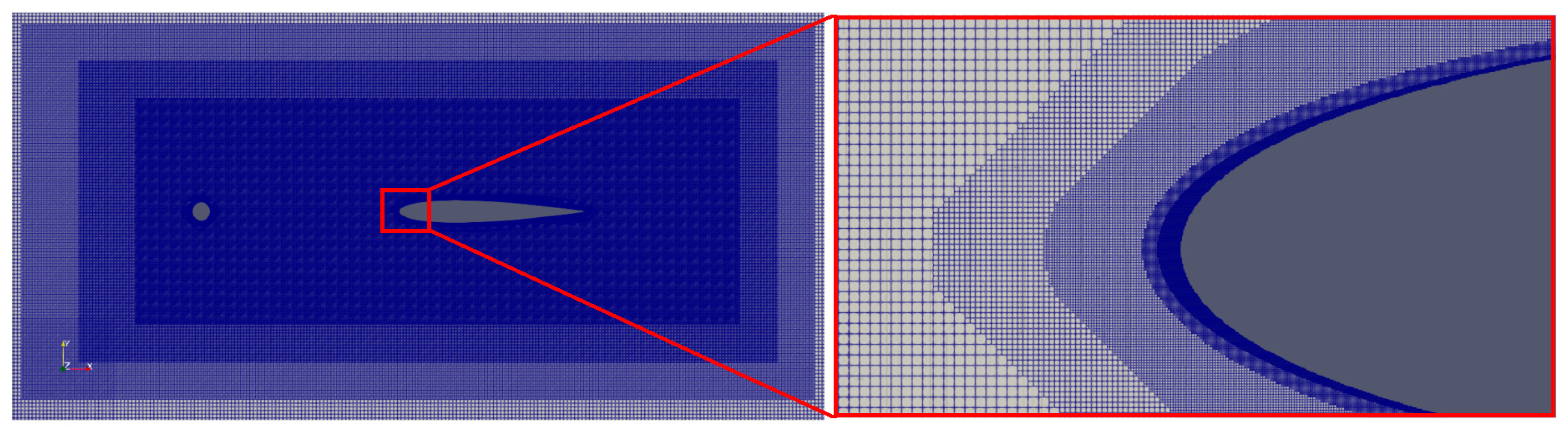
3. Computational Setup

The study by Jacob et al. [1] defines the reference case. In this setup, a NACA0012 airfoil with a chord length of 100 mm and span of 300 mm is used, and a rod is placed at one chord upstream of the airfoil. Two rod diameters, namely 0.01 m and 0.016 m, and four inflow speeds, 30.5, 61, 72, and 115 m/s are experimentally studied. Detailed results are supplied for d = 10 mm and u = 72 m/s (M = 0.21) by the authors; hence, these values are also used for this work for the LES/CAA simulations. The inlet Mach number is M = 0.21, which corresponds to the inlet speed of $U_{\infty }$ = 72 m/s, and the Reynolds number based on the rod and airfoil chord is $R{e}_d$ = 48,000 and $R{e}_c$ = 480,000. Solid surfaces are treated with no-slip boundary conditions, while periodic boundary conditions are imposed in the spanwise direction. The time step size satisfies the Courant number CFL = 1 condition. The spanwise extent of the computational domain is $L_s=0.15c$. The computational domain extends in the streamwise and normal directions, approximately $100d$ rod diameters, as presented in Figure 1.

For the LES/CAA simulations, the coupled FV/DG solver of m-AIA is employed. As mentioned before, the source term used for the CAA simulations is the perturbed lambda vector, which is calculated by using instantaneous and mean parameters. Instantaneous flow parameters are calculated in the coupled simulation at the same time when it is required by the CAA solver, and the mean values are gathered from the mean output file which is obtained by sampling data for a period of time.

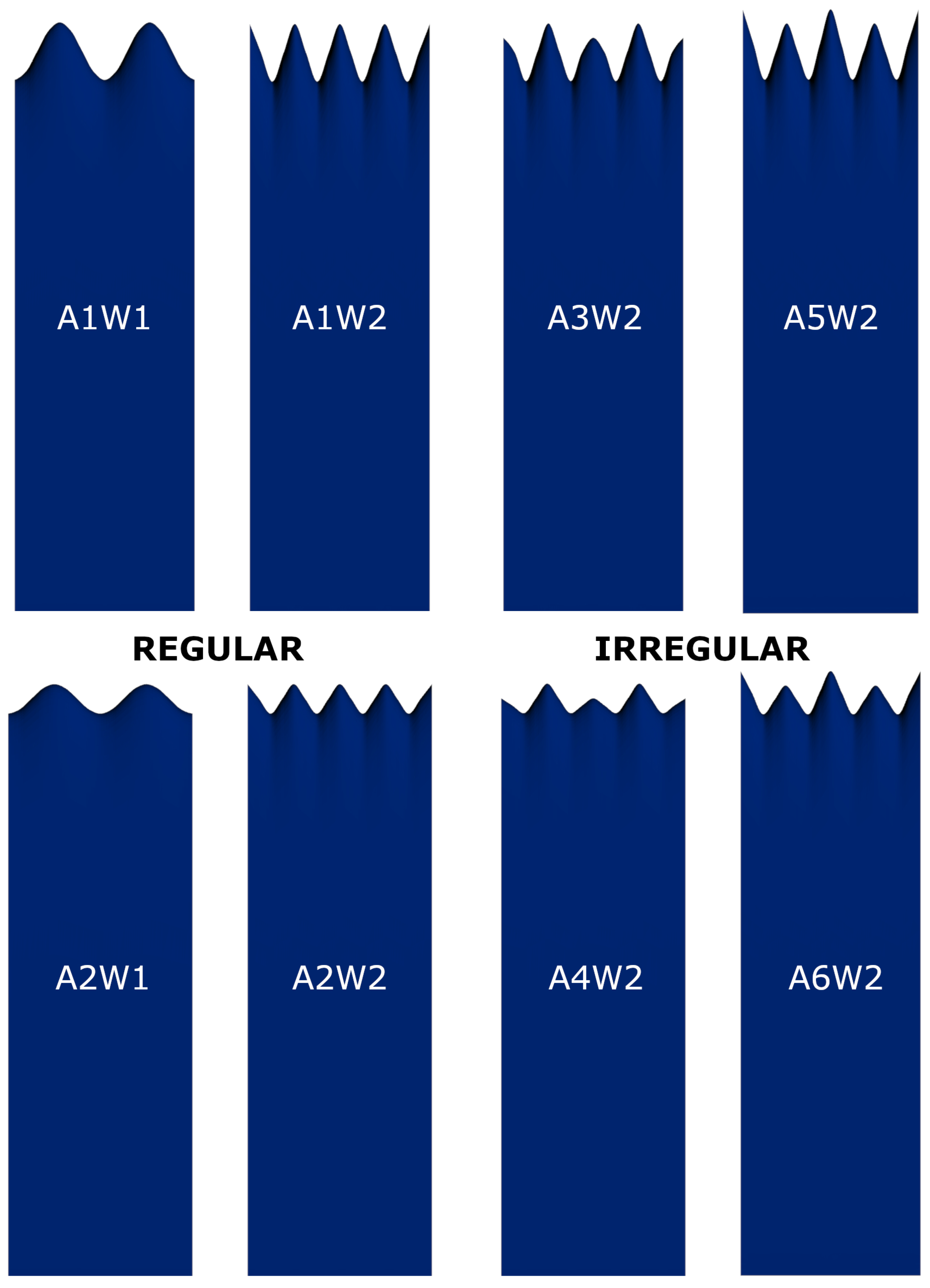
Serrated Leading-Edge Geometries

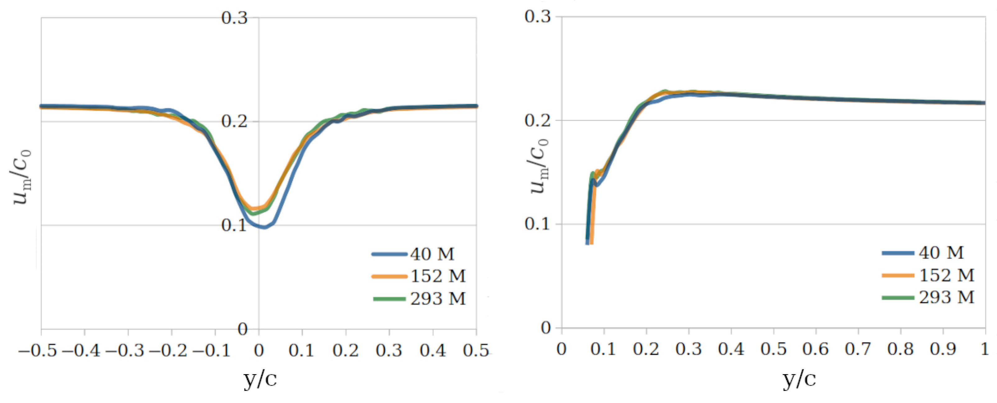
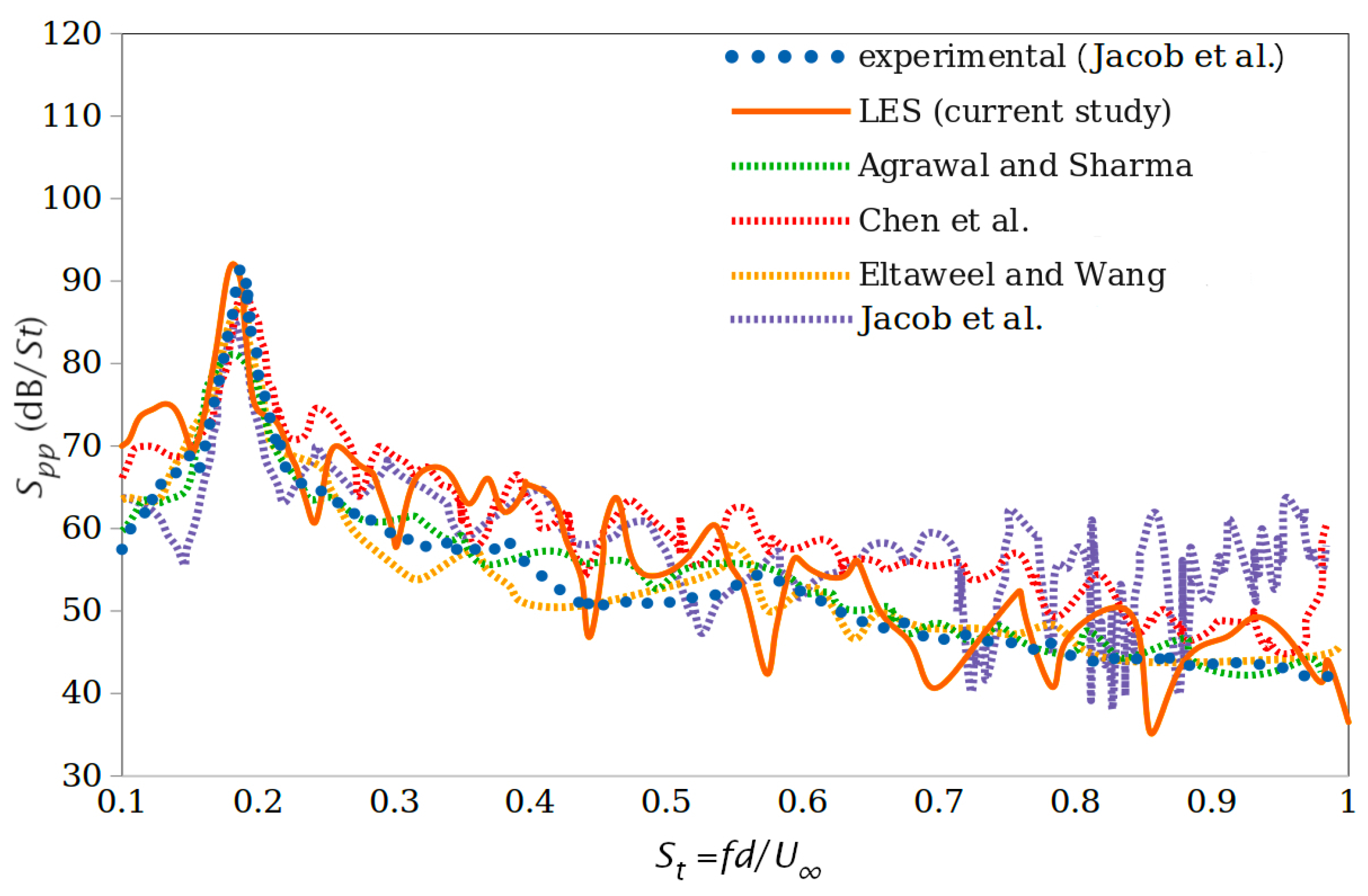
There are various leading-edge treatments for noise mitigation available in the literature [25,26,27]. In this work, regular and irregular serrated trailing edge geometries are tested. The designs with regular serrated leading edges are designed so that the chord length is extended half of the wave length, ensuring a similar wetted area to that of the standard design (STD). New airfoils are designed according to Ref. [11]. The serrated leading-edge airfoil’s chord length in relation to the spanwise coordinate ‘z’ is calculated by Equation (10) where c, A, and W are the chord length, amplitude, and wave length. In the nose region, the coordinates of the standard leading-edge airfoil undergo adjustments based on Equation (11). Specifically, the x coordinates near the nose undergo stretching or contraction in accordance with the spanwise chord length of the serrated leading-edge airfoil, while the coordinates towards the rear remain unaltered [11]. So, y coordinates of the airfoil remain the same, while the new x coordinate ($x_{new}$) is calculated according to the new chord length ($c\left(z\right)$). For instance, for the airfoil with an amplitude of A = 0.1c, the minimum and maximum chord lengths will be 0.95c and 1.05c, respectively. There will also be airfoil sections with chord lengths between these values, whose chord lengths can be calculated according to their span position using Equation (10). After calculating the chord lengths, the $x_{new}$ location is determined using Equation (11). For instance, the new x coordinate where y = 0 for the airfoil with the chord length of 1.05c will be x = 1.05, while it will be x = 0.95 for the airfoil with the chord length 0.95c:

$$c\left(z\right)=c+{\displaystyle \frac{A}{2}}cos\left({\displaystyle \frac{2\pi }{W}}z\right)$$

(10)

$$\left\{\begin{array}{c}{x}_{\mathrm{new}}=\left\{\begin{array}{cc}{\displaystyle \frac{x_{\mathrm{old}}}{x_{max}}}\left[x_{max}+(c\left(z\right)-c)\right]-[c\left(z\right)-c]\hfill & x_{\mathrm{old}}<x_{max}\hfill \\ x_{\mathrm{old}}\hfill & x_{\mathrm{old}}\ge x_{max}\hfill \end{array}\right.\hfill \\ y_{\mathrm{new}}=y_{\mathrm{old}}\hfill \end{array}\right.$$

(11)

In Figure 2, various airfoils utilized in this study are illustrated. Leading edges with regular serrations maintain consistent amplitudes across the span, whereas for the irregular design, amplitudes vary with every second serration, either being increased or reduced by half of the amplitude. The main serration lengths are chosen as 0.025c (A2W1) and 0.05c (A1W1), and the wavelengths between two serration tips are ${\lambda }_{S1}=0.075c$ and ${\lambda }_{S2}=0.0375c$ for the regular designs. In the case of irregular designs, the maximum chord lengths are 1.075c (A3W2), 1.0375c (A4W2), 1.05c (A5W2), and 1.025c (A6W2), while the minimum chord lengths are 1.05c, 1.025c, 1.025c, and 1.0125c, respectively. Illustrations of the regular (left) and irregular (right) serrated leading-edge airfoils are presented in Figure 3.

4. Validation

Three grids containing 40, 152 and 293 million cells are tested for the grid convergence study. The grid is refined around the rod and airfoil to ensure capturing the flow in the boundary layer which is crucial for LES and acoustic simulations. For the grid convergence study, mean x-velocity profiles are collected. Averaging is an important part of this work since the averaged results are also used in CAA simulations. Before starting the averaging process, the simulation is run for nearly $\tilde{t}$ = 86. For averaging, the data are sampled for a period of $\tilde{t}$ = 91, which corresponds to approximately 0.026 s in real time and about 35 shedding periods. Generally, 4096 cores are used for the calculations. The results for the tested grids for two different locations, x = −1.255 and −0.75 as shown in Figure 1 as lines L1 and L2 (TE of the airfoil is the reference, x = 0), are presented in Figure 4. As it can be seen from the figure, the grid with 152 million cells is found to be sufficient for the work. Additionally, the Grid Convergence Index (GCI) is calculated using the minimum and maximum values of the mean streamwise velocity profiles shown in Figure 4. Specifically, the minimum velocity is extracted from line L1 (left plot), and the maximum velocity from line L2 (right plot), for the medium (152M cells) and fine (293M cells) grids. In both cases, the GCI values are below 1%, confirming mesh independence for the selected resolution. The mesh structure of the grid with 152 m cells is presented in Figure 5. As it can be noted from Figure 5, the grid is refined close to the solid bodies. For the validation, the LES results are compared with the experimental data from the study by Jacob et al. [1]. In Figure 6, the LES results of x-component of the velocity distributions at lines L1 and L2 are compared with the experimental data. As seen in the figure, the results are generally in agreement. LES slightly over predicts the reduction in the velocity for the line; however, this is usually the case also for other LES studies like the studies by Agrawal and Sharma [8] and Chen et al. [11]. This could also be due to the y = −2 mm shift between the rod axis and the airfoil chord mentioned in the experimental study [1].

The velocity power spectral density ($S_{uu}$) of the x-velocity plotted against Strouhal number at points P1 and P2 is compared with the experimental and other available results from the literature in Figure 7 [8,11,28]. As it can be seen, the results of the current study are in agreement with the experimental results and also other LES results. The current LES clearly displays the spectral peak and the broadband components.

Finally, the experimental and LES far-field pressure spectral densities (PSD) above the leading edge at 18.5c distance are compared in Figure 8. It can be seen that LES results are in agreement with the experimental measurements. The hybrid LES/CAA model accurately predicts the Strouhal number ($S_t\approx 0.195$) corresponding to the peak $S_{pp}$ value ($S_{pp}\approx 90 dB/St$), with only a slight deviation.

5. Results and Discussion

In the first section of the research results, some results from the flow simulations are presented. The iso-surface of Q-criterion (Q = 1) is given together with an instantaneous contour of x-velocity for the reference case in Figure 9. The vortex street is clear in the wake of the rod and the airfoil is exposed to turbulence. Mean pressure contours for all designs are illustrated across two spanwise sections with the highest and lowest chord lengths for both regular (A1W1, A1W2, A2W1, and A2W2) and irregular (A3W2, A4W2, A5W2, and A6W2) serrations in Figure 10. The mean pressure contours are presented at two spanwise locations, identified as A (left) and B (right) in the bottom-right corner. Each contour is labeled with its configuration name followed by the section identifier (e.g., A1W1-A for configuration A1W1, section A). For the irregular serrations, they are specifically shown on the irregular serration for the highest and lowest chord lengths. This depiction is consistent for regular serrations since they remain the same throughout the span. The highest pressure values ($p_m\approx 0.69$) are observed near the tip of the longest chords, gradually decreasing towards the shortest chords, both for regular and irregular serrations. At the same spanwise locations, contours depicting the mean streamwise ($\overline{u}$) and spanwise ($\overline{v}$) velocity components are illustrated in Figure 11, where mean velocity contours for $\overline{u}$ are presented in the left two columns, while the contours for $\overline{v}$ are shown in the right two columns for the two spanwise locations marked as A and B. The presented figures reveal a discernible influence of serration types on the flow dynamics along the span. Notably, some irregular designs with greater chord lengths, exemplified by A3W2 and A5W2, exhibit slightly heightened velocity magnitudes in comparison to their corresponding regular designs. Conversely, some irregular designs with diminished chord lengths manifest lower velocities than their regular counterparts.

Figure 12 presents the power spectral densities (PSDs) of the streamwise velocity component ($S_{uu}$) at two locations: $x,y=-0.9,0.06$ (left column, subfigures a–c) and $x,y=-0.8,0.07$ (right column, subfigures d–f). Each subplot includes the curves of three configurations: (a, d) show SLE, A1W1, and A1W2; (b, e) show A2W1, A2W2, and A3W2; and (c, f) show A4W2, A5W2, and A6W2. These two points are selected due to their positions on similarly shaped airfoil sections close to the leading edge, taking into account that spanwise sections of each configuration have varying chord lengths along the span. In the proximity of the leading edge, $S_{uu}$ tends to be slightly higher (peak values of nearly $S_{u}u$ $\approx -4$ dB/St) for some irregular serration configurations (e.g., A5W2) compared to their regular counterparts. Notably, the vortex shedding peak exhibits a slight diminishment for some designs such as A1W2, A3W2, and A6W2. This attenuation may be attributed to the improved damping of vortical structures shed by the rod during interaction with the leading edge, resulting in a reduction in noise. Figure 13 displays the power spectral densities (PSDs) of the wall-normal velocity component ($S_{vv}$) at two distinct spanwise locations: $x,y=-0.9,0.06$ (left column, subfigures a–c) and $x,y=-0.8,0.07$ (right column, subfigures d–f). As in the previous figure, each subplot contains the curves of three serration configurations. The highest peak values are approximately $S_{vv}\approx -8 dB/St$ at $x,y=-0.9,0.06$ and $S_{vv}\approx -10 dB/St$ at $x,y=-0.8,0.07$. Similar observations to those of the previous figure can be made here: the reduction in the vortex shedding peak may be causing the reduction in noise levels. Finally, the far-field power spectral density (PSD) of pressure fluctuations is presented for regular (top) and irregular (bottom) leading-edge treatments in Figure 14. The figures on the right provide differences in sound pressure levels, with positive values indicating noise reduction. Notably, all tested configurations demonstrate noise reduction, with the irregular A3W2 and A6W2 designs achieving superior performance—nearly 11 dB reduction in the Strouhal number range of 0.25–0.75. Among the regular serration configurations, designs with higher amplitudes (A1W1 and A1W2) show improved acoustic performance, with reductions reaching up to 10 dB. The A4W2 configuration demonstrates the lowest performance and even shows some noise increase between $St$ = 0.6 and 0.8. The observed low performance of A4W2 may be attributed to its short amplitude characteristics. Specifically, A4W2 possesses a short amplitude similar to that of A2W2, which has been noted to demonstrate inferior noise mitigation performance relative to other variants. This correlation suggests that amplitude length plays a critical role in the effectiveness of noise reduction, with lower amplitudes potentially leading to diminished performance outcomes. At the peak Strouhal ($St$) location, noise reduction is generally modest across all designs, with a notable increase in noise reduction, especially for $St$ > 0.2. The current study observes similar noise reduction characteristics and PSD trends in regular serrated designs to those reported by Chen et al. [11] for comparable serrated airfoil configuration, particularly in terms of amplitude-dependent performance variations. Additionally, these findings are consistent with the observations reported in Yu et al. [29], which indicate that noise reduction performance tends to exhibit a negative correlation with wavelength. It can be seen that the effectiveness of noise mitigation in irregular configurations is influenced by the base amplitude of their regular serration counterparts.

6. Conclusions

This work presents a comprehensive investigation of noise reduction on airfoils with regular and irregular leading-edge serrations subjected to turbulent inflow conditions. Through detailed numerical analysis of the mean pressure fields, velocity components, and power spectral density (PSD) of velocity and pressure fluctuations, irregular geometries are found to produce modified spanwise pressure distributions compared to regular serrations, with higher chord spanwise locations contributing to elevated velocity magnitudes. The results demonstrate that irregular leading-edge serrations A3W2 and A6W2 achieve superior noise reduction performance, reaching up to 11 dB in the Strouhal range St = 0.25–0.75. Among regular serration configurations, high-amplitude designs A1W1 and A1W2 achieve up to 10 dB reduction. The A4W2 configuration demonstrate the lowest performance and even shows noise increase between St = 0.6 and 0.8, which may be attributed to its short amplitude characteristics, similar to A2W2, which has been observed to demonstrate inferior noise mitigation performance relative to other variants. This relationship suggests that amplitude length plays an important role in the effectiveness of noise reduction, with shorter amplitudes potentially leading to diminished performance outcomes. Additionally, it is observed that noise reduction tends to exhibit a negative correlation with wavelength parameters. The study reveals that the noise reduction effectiveness of irregular configurations is influenced by the base amplitude of their regular serration counterparts. These findings indicate that irregular serrations possess the capacity to achieve considerable noise reduction. Consequently, it is likely that noise reduction levels could be further enhanced with alternative irregular serration designs.

References

1. Jacob, M.C.; Boudet, J.; Casalino, D.; Michard, M. A Rod-Airfoil Experiment as a Benchmark for Broadband Noise Modeling. Theor. Comput. Fluid Dyn. 2005, 19, 171–196. [Google Scholar] [CrossRef]
2. Moore, P.; Lorenzoni, V.; Scarano, F. Two Techniques for PIV-Based Aeroacoustic Prediction and Their Application to a Rod-Airfoil Experiment. Exp. Fluids 2010, 50, 877–885. [Google Scholar] [CrossRef]
3. Giret, J.-C.; Sengissen, A.; Moreau, S.; Sanjose, M.; Jouhaud, J.-C. Noise Source Analysis of a Rod-Airfoil Configuration Using Unstructured Large-Eddy Simulation. AIAA J. 2015, 53, 1062–1077. [Google Scholar] [CrossRef]
4. Li, Y.; Wang, X.; Chen, Z.; Zheng-chu, L. Experimental Study of Vortex-Structure Interaction Noise Radiated from Rod-Airfoil Configurations. J. Fluid Struct. 2014, 51, 313–325. [Google Scholar] [CrossRef]
5. Jiang, M.; Li, X.; Zhou, J. Experimental and Numerical Investigation on Sound Generation from Airfoil-Flow Interaction. Appl. Math. Mech. 2011, 32, 765–776. [Google Scholar] [CrossRef]
6. Jiang, Y.; Mao, M.-L.; Deng, X.-G.; Liu, H.-Y. Numerical Investigation on Body-Wake Flow Interaction Over Rod-Airfoil Configuration. J. Fluid Mech. 2015, 779, 1–35. [Google Scholar] [CrossRef]
7. Sharma, S.; Geyer, T.F.; Giesler, J. Effect of Geometric Parameters on the Noise Generated by Rod-Airfoil Configuration. Appl. Acoust. 2021, 177, 107908. [Google Scholar] [CrossRef]
8. Agrawal, B.R.; Sharma, A. Numerical Analysis of Aerodynamic Noise Mitigation via Leading Edge Serrations for a Rod-Airfoil Configuration. Int. J. Aeroacoust. 2016, 15, 734–756. [Google Scholar] [CrossRef]
9. Chen, W.; Qiao, W.; Tong, F.; Wang, L.; Wang, X. Experimental Investigation of Wavy Leading Edges on Rod-Aerofoil Interaction Noise. J. Sound Vib. 2018, 422, 409–431. [Google Scholar] [CrossRef]
10. Fan, T.; Qiao, W.; Chen, W.; Cheng, H.; Wei, R.; Wang, X. Numerical Analysis of Broadband Noise Reduction with Wavy Leading Edge. Chin. J. Aeronaut. 2018, 31, 1489–1505. [Google Scholar]
11. Chen, W.; Qiao, W.; Tong, F.; Wang, L.; Wang, X. Numerical Investigation of Wavy Leading Edges on Rod-Airfoil Interaction Noise. AIAA J. 2018, 56, 2553–2567. [Google Scholar] [CrossRef]
12. Teruna, C.; Avallone, F.; Casalino, D.; Ragni, D. Numerical Investigation of Leading Edge Noise Reduction on a Rod-Airfoil Configuration Using Porous Materials and Serrations. J. Sound Vib. 2021, 494, 115880. [Google Scholar] [CrossRef]
13. Chen, W.; Lei, H.; Xing, Y.; Wang, L.; Zhou, T.; Qiao, W. On the airfoil leading-edge noise reduction using poro-wavy leading edges. Phys. Fluids 2024, 36, 035158. [Google Scholar] [CrossRef]
14. Wang, Y.; Tong, F.; Chen, Z.; Wang, C.; Jiang, S. Rod–Airfoil Interaction Noise Reduction Using Gradient Distributed Porous Leading Edges. Appl. Sci. 2022, 12, 4941. [Google Scholar] [CrossRef]
15. Gao, R.; Chen, W.; Tong, H.; Zhang, Y.; Zhang, L.; Wang, X.; Qiao, W. Aerodynamic performance of a fan with porous-wavy leading edge. Phys. Fluids 2025, 37, 047128. [Google Scholar] [CrossRef]
16. Yu, F.-Y.; Wan, Z.-H.; Hu, Y.-S.; Sun, D.-J.; Lu, X.-Y. Effects of leading-edge serration shape on noise reduction in rod-airfoil interactions. J. Acoust. Soc. Am. 2025, 157, 215–233. [Google Scholar] [CrossRef]
17. Paruchuri, C.C.; Narayanan, S.; Joseph, P.; Kim, J.W. Leading Edge Serration Geometries for Significantly Enhanced Leading Edge Noise Reductions. In Proceedings of the 22nd AIAA/CEAS Aeroacoustics Conference, Lyon, France, 30 May–1 June 2016; p. 2736. [Google Scholar]
18. Schlottke-Lakemper, M.; Yu, H.; Berger, S.; Meinke, M.; Schröder, W. A Fully Coupled Hybrid Computational Aeroacoustics Method on Hierarchical Cartesian Meshes. Comput. Fluids 2017, 144, 137–153. [Google Scholar] [CrossRef]
19. Institute of Aerodynamics. m-AIA, 2024, 13350586. Available online: https://doi.org/10.5281/zenodo.13350586 (accessed on 20 October 2024).
20. Boris, J.P.; Grinstein, F.F.; Oran, E.S.; Kolbe, R.L. New Insights into Large Eddy Simulation. Fluid Dyn. Res. 1992, 10, 199. [Google Scholar] [CrossRef]
21. Van Leer, B. Towards the Ultimate Conservative Difference Scheme. V. A Second-Order Sequel to Godunov’s Method. J. Comput. Phys. 1979, 32, 101–136. [Google Scholar] [CrossRef]
22. Schneiders, L.; Günther, C.; Meinke, M.; Schröder, W. An Efficient Conservative Cut-Cell Method for Rigid Bodies Interacting with Viscous Compressible Flows. J. Comput. Phys. 2016, 311, 62–86. [Google Scholar] [CrossRef]
23. Cetin, M.O.; Koh, S.R.; Meinke, M.; Schröder, W. Numerical Analysis of the Impact of the Interior Nozzle Geometry on Low Mach Number Jet Acoustics. Flow Turbul. Combust. 2017, 98, 417–443. [Google Scholar] [CrossRef]
24. Ewert, R.; Schröder, W. Acoustic Perturbation Equations Based on Flow Decomposition via Source Filtering. J. Comput. Phys. 2003, 188, 365–398. [Google Scholar] [CrossRef]
25. Xiao, C.; Tong, F. Experiment on Noise Reduction of a Wavy Cylinder with a Large Spanwise Wavelength and Large Aspect Ratio in Aeroacoustic Wind Tunnels. Appl. Sci. 2023, 13, 6061. [Google Scholar] [CrossRef]
26. Wang, Y.; Zuo, K.; Guo, P.; Zhao, K.; Kopiev, V.F. Experimental Investigation of Airfoil Instability Tonal Noise Reduction Using Structured Porous Trailing Edges. Appl. Sci. 2024, 14, 2992. [Google Scholar] [CrossRef]
27. Al-Okbi, Y.; Chong, T.P.; Stalnov, O. Leading Edge Blowing to Mimic and Enhance the Serration Effects for Aerofoil. Appl. Sci. 2021, 11, 2593. [Google Scholar] [CrossRef]
28. Eltawcel, A.; Wang, M. Numerical Simulation of Broadband Noise from Airfoil-Wake Interaction. In Proceedings of the 17th AIAA/CEAS Aeroacoustics Conference (32nd AIAA Aeroacoustics Conference), Portland, OR, USA, 5–8 June 2011; p. 2802. [Google Scholar]
29. Yu, F.-Y.; Wan, Z.-H.; Hu, Y.-S.; Sun, D. Effects of the wavy leading-edge wavelength on the reduction in the noise of the rod–airfoil configuration. JUSTC 2025, 55, 0202. [Google Scholar] [CrossRef]
Figure 1. General view of the computational domain and locations of measurement points and lines.
Applsci 15 07822 g001
Figure 2. Illustration of some airfoil geometries: The A1W1 configuration features regular serrations with a 0.05c amplitude, producing chord lengths between 0.95c and 1.05c, while the A2W1 configuration has regular serrations with a 0.025c amplitude, yielding chord lengths between 0.975c and 1.025c. The irregular A5W2 and A6W2 designs alternate serration amplitudes by ±50% of their base values (0.05c and 0.025c respectively), creating asymmetric chord distributions.
Applsci 15 07822 g002
Figure 3. Airfoils with regular (left) and irregular (right) LE serrations: Regular serrations maintain a constant amplitude across the span, whereas irregular geometries alternate the amplitude of every second serration by ±50% of their base values.
Applsci 15 07822 g003
Figure 4. Mean x-velocity profiles at lines L1 (left) and L2 (right).
Applsci 15 07822 g004
Figure 5. Mesh structure.
Applsci 15 07822 g005
Figure 6. Comparison of mean streamwise velocity (u) profiles at lines L1 (left) and L2 (right), showing the current LES results alongside experimental data by Jacob et al. [1] and previous LES studies by Agrawal and Sharma [8] and Chen et al. [11].
Applsci 15 07822 g006
Figure 7. Power spectral density ( S u u ) of the streamwise velocity (u) plotted against the Strouhal number at points P1 and P2, showing results from the current LES, experimental data by Jacob et al. [1], and previous LES studies by Agrawal and Sharma [8], Chen et al. [11], and Eltawcel and Wang [28].
Applsci 15 07822 g007
Figure 8. Comparison of far-field pressure spectral densities above the airfoil leading edge at 18.5c distance, showing results from the current LES, both experimental and LES data by Jacob et al. [1], and previous LES studies by Agrawal and Sharma [8], Chen et al. [11], and Eltawcel and Wang [28].
Applsci 15 07822 g008
Figure 9. The iso-surfaces of Q-criterion (Q = 1) with instantaneous contour of x-velocity.
Applsci 15 07822 g009
Figure 10. Mean pressure contours at two spanwise locations, marked by red dashed lines in the bottom-right corner as A (left) and B (right) on each configuration. All contours are labeled with their configuration name followed by the section identifier (e.g., A1W1-A for configuration A1W1, section A).
Applsci 15 07822 g010
Figure 11. Mean velocity contours, u m (left, first two columns) and v m (right, third and fourth columns), at two spanwise locations, marked by red dashed lines in the bottom-left (A1W1, A1W2, A2W1, and A2W2) and bottom-right (A3W2, A4W2, A5W2, and A6W2) corners as A (left) and B (right) on each configuration. All contours are labeled with their configuration name followed by the section identifier (e.g., A1W1-A for configuration A1W1, section A).
Applsci 15 07822 g011
Figure 12. PSD of u velocity ( S u u ) at ( x , y ) = ( 0.9 , 0.06 ) (ac) and at ( x , y ) = ( 0.8 , 0.07 ) (df) for different serration configurations: (a,d) SLE, A1W1, A1W2; (b,e) A2W1, A2W2, A3W2; (c,f) A4W2, A5W2, A6W2. The reference is 1 m 2 s 2 . The leading and trailing edges of the reference design are located at ( x , y ) = ( 1.0 , 0.0 ) and ( x , y ) = ( 0.0 , 0.0 ) , respectively.
Applsci 15 07822 g012
Figure 13. PSD of v velocity ( S v v ) at ( x , y ) = ( 0.9 , 0.06 ) (ac) and at ( x , y ) = ( 0.8 , 0.07 ) (df) for different serration configurations: (a,d) SLE, A1W1, A1W2; (b,e) A2W1, A2W2, A3W2; (c,f) A4W2, A5W2, A6W2. The reference is 1 m 2 s 2 . The leading and trailing edges of the reference design are located at ( x , y ) = ( 1.0 , 0.0 ) and ( x , y ) = ( 0.0 , 0.0 ) , respectively.
Applsci 15 07822 g013
Figure 14. PSD of pressure fluctuations for (a) regular and (b) irregular leading-edge treatments. Sound pressure level differences are provided in the figures (c,d) (positive values indicate noise reduction).
Applsci 15 07822 g014