Automated Modal Analysis Using Stochastic Subspace Identification and Field Monitoring Data

Abstract

The accurate identification of modal parameters is essential for structural health monitoring (SHM), as it provides critical insights into the presence of damage or degradation within the structure. A promising technique, stochastic subspace identification (SSI) has numerous advantages in operational modal analysis (OMA), particularly in implementing automated OMA. Hence, an improved procedure is proposed in this study, addressing the size of the SSI matrix, the estimation of system order, and the removal of spurious modes for automated modal analysis. A general instruction for user-defined parameters is first reviewed and summarized. Subsequently, a proposed procedure is then introduced and framed into three steps. Key advances include the preliminary identification of fundamental frequency, which helps the overall automated work, adequately assigning the size of the SSI matrix, which can improve decomposition, and a decay function, which provides a good estimation of system order. To demonstrate and verify the procedure, a numerical simulation of a ten-story shear-type building structure and two field datasets, collected from reinforced concrete (RC) frames in Taiwan, are utilized. Consequently, the results suggest that the proposed three-step procedure based on SSI can facilitate automated OMA for continuous and long-term SHM, in terms of autonomously adjusting user-defined parameters.

1. Introduction

Modal parameters, such as natural frequency, damping ratio, and mode shape, reflect structures’ fundamental behaviors and dynamic characteristics. Hence, the accurate identification of modal parameters is essential for structural health monitoring (SHM), as it provides critical insights into the presence of damage or degradation within the structure [1,2].

Currently, two primary approaches are commonly used to identify modal parameters from structures: experimental modal analysis (EMA) and operational modal analysis (OMA). EMA involves applying known excitations, typically using mechanical shakers or impact hammers, and measuring the resulting responses with sensors, such as accelerometers [3,4]. Generally, frequency response functions obtained from these structural responses are then analyzed using techniques, such as curve fitting or system identification techniques, to extract the modal parameters. In contrast, OMA estimates modal parameters solely from the structural responses measured in the ambient environment, without the need for controlled excitations [5,6]. Certainly, this approach is especially advantageous for continuous and long-term SHM, and is particularly applicable to complex structures or field applications, where applying controlled excitations is difficult or impractical.

In past decades, OMA has seen significant advancements, with numerous methods developed and successfully applied to civil structures. These identification techniques are broadly categorized into frequency-domain approaches and time-domain approaches [7,8,9]. Specifically, the first analyzes measured responses in the spectral domain and the latter directly analyzes them over time. For instance, frequency-domain approaches include peak-picking on the power spectrum, frequency-domain decomposition (FDD), enhanced FDD, Bayesian fast Fourier Transform (FFT), Bayesian spectral density, the Gaussian mixture model, and so on [10,11]. Recently, innovations in signal processing and system identification techniques have driven the evolution of time-domain OMA [1,12]. For example, the random decrement technique estimates free vibration behavior from ambient or noisy measurements. Similarly, the natural excitation technique (NExT) isolates free vibration responses from forced responses under unknown excitations. Autoregressive models, such as autoregressive moving average (ARMA), predict output responses using past values to infer modal properties. Methods based on cross-power spectrum analysis identify modal parameters by examining frequency content and phase relationships between output signals. Moreover, the eigensystem realization algorithm (ERA) constructs state–space models and derives modal parameters from state–matrix eigenvalues. Last but not least, stochastic subspace identification (SSI) stands out for its ability to process large datasets and robustness against noise, eliminating the need for free-decay signals or cross-correlation functions.

Among the time- and frequency-domain approaches available for OMA, SSI, in particular, has gained prominence due to its versatility in handling real-world structural monitoring challenges. Other advantages include the ability to process large datasets, applicability to linear systems, and inherent robustness against measurement noise and disturbances [13,14]. Fundamental work on subspace-related methods was first carried out by Leopold Kronecker, a German mathematician, in 1890 [15]. Its solid mathematical basis was built on by a number of researchers—such as Ho and Kalman, Youla and Tissi, and so on—to exploit the Markov parameters of linear systems in the 1960s [15]. Then, some breakthroughs were made by Van Overschee and De Moor, who systematically formulated the state–space-based method, discreetly developed theoretical frameworks to eliminate reliance on input measurements, and thoughtfully established implementation guidelines for the identification process [16,17,18]. Consequently, two common alternatives to SSI have been developed, which differ in terms of how they treat data [19,20]. One is data-driven SSI (SSI-Data), which directly uses measured responses without special processing; the other is covariance-driven SSI (SSI-Cov), which requires that a covariance matrix be first computed from measured responses and then utilized for identification. Thereafter, a number of researchers further refined SSI methodologies: Kvåle et al. looked over SSI-Cov, SSI-Data, and frequency-domain decomposition for bridge monitoring, with SSI-Cov delivering superior accuracy [21,22]; Priori et al. established guidelines for selecting user-defined parameters in SSI-Data, addressing both stationary and non-stationary excitation conditions [23]; Li et al. analyzed the influences of parameters on SSI-Cov for arch dam monitoring, providing practical recommendations for optimal parameter selection [24]; and so on [25,26]. As famous output-only approaches, these methodologies have seen widespread adoption across civil engineering (e.g., dams, bridges), mechanical systems, and aerospace structures, underscoring their versatility and robustness.

Assuredly, SSI has numerous applications in OMA, which offer modal analysis in ambient environments [27,28,29]. However, recently, there has been increasing interest in implementing automated OMA, which works as a cornerstone of streamlining long-term SHM by minimizing human intervention [30,31]. The newest researchers are therefore attempting to integrate artificial intelligence (AI) [32,33]. Nevertheless, this implementation faces specific challenges and emergent enhancements [34]. For example, one limitation is the requirement to manually specify the model order during field monitoring, as estimating system order accurately is often difficult [35]. To address this, practitioners frequently over-specify the order to improve data fitting accuracy, but this risks introducing spurious modes into the results [36]. The stabilization diagram has been exploited as a critical tool for distinguishing physical modes from spurious ones by varying parameters and identifying stable vertical lines. Despite their utility, interpreting these diagrams still relies on human expertise. To enable full automation, researchers employ a pre-filtering method, which applies criteria such as Modal Phase Collinearity (MPC) to eliminate obvious outliers [37,38]. Instead, one can cluster modes with similar dynamic characteristics using grouping algorithms, such as partition-based clustering, density-based clustering, and so on and so forth [39,40]. While these methods enhance automation, their effectiveness hinges on the robustness of logical rules and thresholds in diverse scenarios. A persistent issue arises for complex structures or field applications, where residual spurious poles (outliers) evade prefiltering and disrupt clustering accuracy, ultimately compromising the reliability of modal analysis.

This study aims to propose an improved procedure for implementing automated OMA based on SSI, focusing specifically on the selected size of the SSI matrix, the estimation of system order, and the removal of spurious modes. To facilitate a long-term SHM using SSI, a comprehensive discussion is addressed across data preprocessing, matrix construction, numerical decomposition, and system realization. The rest of this paper is structured as follows. First, the basic formulation of SSI is introduced and derived to illustrate the overall procedure for implementing automated OMA. A general instruction for user-defined parameters, used while applying SSI, is also reviewed and summarized. Subsequently, according to the discussion on adequate user-defined parameters, an improved procedure is proposed and framed into three steps. Some key examinations are numerically demonstrated using a simulation study of a shear-type building structure. To verify the automated SSI-based OMA for long-term SHM, two datasets extracted from the field applications are investigated and analyzed in this study. Both datasets contain acceleration responses collected from the reinforced concrete (RC) frames in Taiwan, and they all have time-varying dynamic characteristics, included over a decade of data. In the examples, fundamental frequency and the adequate size of the SSI matrix, introduced by the proposed procedure, remove the need to interpret the stabilization diagram and the appearance of spurious modes. The decay function provides an indicator for system order in field applications and facilitates automated OMA. Furthermore, the proposed procedure is briefly concluded, noting that cross-verification of automated SSI-based OMA for long-term SHM may still be necessary.

2. Subspace Identification

The numerical algorithms for subspace state space system identification (N4SID) have gained increasing attention in the field of system identification [16,17,18]. The advantages of N4SID include easy implementation, the requirement for less prior knowledge, high compatibility, versatile applications, and so on. In the following derivation, matrices and vectors are represented using bold font, while scalars are represented using italic font. Considering a generic stochastic excitation sampled as a time interval equal to Dt, the state–space formulation of a linear time-invariant (LTI) structural system with a degree-of-freedom (DOF) n is:

$$x_{k+1}=A{x}_k+w_k$$

(1)

$$y_k=C{x}_k+v_k$$

(2)

where x_k (2n × 1) is the discrete state at the k-th step, y_k (m × 1) is the measured response, and m indicates the number of measurements. The discrete-time state is usually composed of structural displacement and structural velocity; on the contrary, the measured response is usually composed of structural acceleration in the ambient environment. w_k and v_k represent the system and measurement noise at the k-th step, respectively; they are assumed to be stationary and zero-mean random processes. Additionally, state–space matrices A and C represent the state (or system) matrix and output matrix, respectively. Unquestionably, the above equations form the background for SSI.

2.1. Implementation of Stochastic Subspace Identification (SSI)

SSI begins with the arrangement of the block Hankel matrix, H, as

$$H={\displaystyle \frac{Y_p}{Y_f}}={\displaystyle \frac{\left[\begin{array}{cccc}{y}_{1\hspace{0.33em}|\hspace{0.33em}i}& y_{2\hspace{0.33em}|\hspace{0.33em}i+1}& \dots & y_{j\hspace{0.33em}|\hspace{0.33em}i+j-1}\end{array}\right]}{\left[\begin{array}{cccc}{y}_{i+1\hspace{0.33em}|\hspace{0.33em}2i}& y_{i+2\hspace{0.33em}|\hspace{0.33em}2i+1}& \dots & y_{i+j\hspace{0.33em}|\hspace{0.33em}2i+j-1}\end{array}\right]}}$$

(3)

where the lagged vectors are arranged as

$$y_{1\hspace{0.33em}|\hspace{0.33em}i}={\left[\begin{array}{cccc}{y}_1^T& y_2^T& \dots & y_i^T\end{array}\right]}^T$$

(4)

It is clear that the block Hankel matrix is split into two partitions; Y_p and Y_f are the past and future output Hankel matrix, respectively. From Equation (3), it is obvious that the total number of samples is equal to $2i+j-1$.

Then, the state (or system) matrix and output matrix can be inversely computed through the orthogonal projection, which projects the row space of the future outputs onto the row space of the past outputs.

$$O_{\mathrm{orth}}=Y_f{Y}_p^T{(Y_p{Y}_p^T)}^{†}{Y}_p$$

(5)

This approach is known as SSI-Data. Alternatively, these state–space matrices can be inversely computed through the covariance matrix.

$$O_{\mathrm{cov}}=Y_f{Y}_p^T$$

(6)

This approach is known as SSI-Cov. The column space of both approaches yields the extended observability matrix, constituting with A and C. Hence, singular value decomposition (SVD) can be used to decompose the matrix as

$$O=US{V}^T=\left[\begin{array}{cc}{U}_1& U_2\end{array}\right]\left[\begin{array}{cc}{S}_1& 0\\ 0& S_2\end{array}\right]\left[\begin{array}{c}{V}_1^T\\ V_2^T\end{array}\right]\approx U_1{S}_1{V}_1^T$$

(7)

where the dimension of S₁ reveals the order of the structural system (2n), and can be specified, at least theoretically, by considering the non-zero singular values of O. Understandably, S₂ consists of the zero singular values of O.

Finally, SSI ends with its shift invariance property. The state (or system) matrix and output matrix characterizing the LTI structural system can be estimated as

$$C=U_1(1:m,\hspace{0.33em}:)$$

(8)

$$A=U_1^{†}(1:im-m,\hspace{0.33em}:)U_1(m+1:im,\hspace{0.33em}:)$$

(9)

Once the state–space matrices are estimated, the identification of the modal parameters is then straightforward for the structural system.

2.2. General Instruction for User-Defined Parameters

The initial and unavoidable step before the implementation of SSI is to select the user-defined parameters. These parameters can be roughly categorized into three parts: the size of the Hankel matrix, the estimation of system order, and the criterion of assured modes. Fortunately, researchers have carried out comprehensive studies and provided valuable suggestions in the past few years [23,41].

2.2.1. Size of the Hankel Matrix

The number of rows, i, and columns, j, is one parameter for establishing the block Hankel matrix. However, it can be observed from Equation (3) that the total number of samples is equal to $2i+j-1$, so the column number can be uniquely defined if the row number, i, is selected.

The maximum value of the row number, i, is not explicitly restricted, although a large value may frustrate the identification of high-frequency modes because of their relatively small energy. Oppositely, the minimum value has some rules of thumb; for example, the row number, i, multiplied by the number of measurements, m, needs to be equal to or larger than the system order according to the Cayley–Hamilton theorem [19], which implies.

$$im\ge 2n$$

(10)

Furthermore, the samples used in the rows or columns must cover the fundamental frequency (or lowest frequency) of the structural system, f₀. Some studies recommend $i\ge 1/f_0\mathsf{\Delta }t$ for lagged vectors by considering a complete cycle [24,42], while others recommend $2i\ge 1/f_0\mathsf{\Delta }t$ for considering the Nyquist frequency [43,44].

2.2.2. Estimation of System Order

The dimension of S₁ is another user-defined parameter representing the estimation of system order, and it is crucial while implementing SSI. In the case of complex structures or field applications, the distinguishment between non-zero but small singular values and zero singular values is vague. An obvious number of spurious modes can be generated if a larger value is selected. However, if a smaller value is assumed as the representing system order, the modes with relatively low energy may be lost during realization.

Estimating system order was first addressed in the 2000s in the context of sub–space methods [45]. Three different approaches can be utilized; two use the information hidden in the singular values, while the third employs estimated innovation variance. For example, one approach estimates system order according to the magnitudes of singular values while dealing with a time-varying system [46]. Following a similar thought, another approach estimates it by adjusting an adequate ratio of the first (largest) singular value as a criterion [47]. A slightly more advanced approach exploits the difference between each singular pair, and this approach compares the information with the signal-to-noise ratio (SNR), providing a more realistic way for choosing a system order [44], despite the fact that this approach is more sophisticated. One recent approach uses variance accounting for (VAF) as a criterion to estimate system order, and this approach ensures that reconstructed responses under the estimated system order can be easily retrieved [41].

2.2.3. Criterion of Assured Modes

In field applications, the modes identified by subspace methods can be affected by many factors. For instance, uncertainties, environmental effects, process noise, and measurement noise can lead to unstable and spurious poles. Differentiating assured modes from others is crucial, after applying Equations (8) and (9), to realizing structural systems. A simple way to sieve out these assured modes is to select stable (or invariable) identified parameters regarding the dynamic characteristics in a stability diagram. One of the easiest methods is proposing thresholds to limit variations of modal frequencies, damping ratios, and mode shapes [48]. However, a nonlinear or time-variant structural system naturally generates variable modal parameters, which, though minor, violate the invariable identification results.

A substitute is to compare identified mode shapes using MPC, modal assurance criterion (MAC), modal complexity factor (MCF), and so on. Regardless, Vacher et al. had evidenced that MPC is nothing more than MAC evaluated using identified mode shapes and their conjugate shapes [49]. Additionally, a few derivations can demonstrate the apparent similarity between MPC and MCF, as shown below

$$S_{xx}={\Phi }_r^T{\Phi }_r,\hspace{1em}{S}_{yy}={\Phi }_i^T{\Phi }_i,\hspace{1em}{S}_{xy}={\Phi }_r^T{\Phi }_i,$$

(11)

$$MPC(\Phi )={\displaystyle \frac{{(S_{yy}-S_{xx})}^2+4S_{xy}^2}{{(S_{yy}+S_{xx})}^2}}=1-MCF(\Phi )$$

(12)

where Φ is the identified mode shapes, and the subscripts r and i denote the real and imaginary parts of the complex vectors, respectively. Therefore, MAC is recommended in this study to differentiate assured modes from others.

3. Proposed Procedure

To implement SSI while considering adequate user-defined parameters for automated OMA, three steps are proposed instead of constructing the block Hankel matrix straightforwardly after the measurements are collected. In particular, spurious modes and unsteady stability diagrams dramatically affect identification results in field applications. These steps include data preprocessing, matrix construction and decomposition, and system realization, as shown in Figure 1. Herein, the proposed procedure is numerically illustrated using a simulation study of a shear-type building structure. The fundamental frequency (or lowest frequency), f₀, is assigned as 1 Hz, and the damping ratios of the structural system for all modes are assigned as 2%. To focus on the effectiveness of the procedure, the measurements are assumed to be noiseless and the full measurement is sampled with 50 Hz.

3.1. Data Preprocessing

SSI is assumed to be stochastically excited by stationary and zero-mean random processes. Therefore, at the very beginning, measurements need to be confirmed, provided they are collected under similar assumptions, to excite the structure’s modes of interest. If the measurements are mainly acquired during nonstationary events, some techniques can be helpful to differentiate nonstationary excitations. Such techniques include short-time average through long-time average (STA/LTA), normalized Arias intensity, Akaike information criterion (AIC), and so on. For example, Figure 2a,b demonstrates how normalized Arias intensity and AIC determine the initial time of a seismic event. AIC estimates the relative amount of information lost by statistical models, while normalized Arias intensity computes amplitude changes across the time axis. These techniques are generally called P-wave pickers. Once the nonstationary excitations are determined, only the measured response outside nonstationary events can be used to construct the block Hankel matrix.

Next, the fundamental frequency (or lowest frequency) of the structural system needs to be roughly determined using FFT, and in the meantime, the structure’s modes of interest can be checked. Moreover, the SNR can also be conjectured to assess noise levels in measurements. As stated in Section 2, fundamental frequency is crucial for choosing the size of the Hankel matrix, and the overview of the structure’s modes provides advantageous information about the representing system order, which is useful for choosing the system order and reducing the computational effort. Similarly, Figure 2c demonstrates how FFT provides the most basic signal and modal information before the automated SSI-based OMA is applied. Consequently, the measurements can be down-sampled once the Nyquist frequency is significantly higher than the structure’s modes. The fundamental frequency can be estimated through the Fourier spectrum. Notably, signal and modal information can also be found by other data-driven techniques, i.e., wavelet transform. However, FFT is obviously the best technique because of its few assumptions and less computational effort.

3.2. Matrix Construction and Decomposition

Admittedly, the size of the Hankel matrix is based on fundamental frequency, and $2i\ge 1/f_0\mathsf{\Delta }t$ is the minimal value to take into account for the Nyquist frequency. The choice of size of the Hankel matrix can affect the resultant decomposition performed by SVD. Theoretically, a non-centering (non-zero-mean) Hankel matrix does not inherently destabilize SVD; however, large mean values can dominate the decomposition, leading to reduced sensitivity or poorer low-rank approximations. Moreover, singular vectors and singular values often align with the dominant direction, which may include mean values if the Hankel matrix is not centering. A similar phenomenon can be found even if the responses of only a few modes are not zero-mean. For example, Figure 3a demonstrates singular values decomposed using different sizes of Hankel matrix. The singular values are unclearly decomposed when i = 31 and i = 36. Obviously, an inappropriate size choice makes the lagged vectors non-centering and eventually disturbs the distribution of singular values.

On the contrary, the phenomenon can be mitigated once a zero-mean modal response is secured, especially the fundamental mode. Considering that vibration modes are represented in singular values as pairs, the normalized differences between singular pairs are defined as

$${\sigma }_{\mathrm{diff},p}=2\cdot {\displaystyle \frac{{\sigma }_{2p}-{\sigma }_{2p+1}}{{\sigma }_{2p}+{\sigma }_{2p+1}}}\hspace{1em}p=0,\hspace{0.33em}1,\hspace{0.33em}2,\dots$$

(13)

Figure 3b–d show the normalized differences between the first three singular pairs after implementing SSI-Data. The largest differences can be observed around the bottom left where $2i\ge 1/f_0\mathsf{\Delta }t$ is unsatisfied. Clearly, they wave across the size of the Hankel matrix, indicating that only some numbers of rows can bring about clear decomposition with very few differences. Notably, similar observations can be found after implementing SSI-Cov, although this is as significant as implementing SSI-Data. Figure 3e shows normalized differences between the first singular pair accompanied by the integer multiples of the fundamental periods as

$$i=\mathrm{nint}\left({\displaystyle \frac{p}{2f_0\mathsf{\Delta }t}}\right)\hspace{1em}p=1,\hspace{0.33em}2,\hspace{0.33em}3,\dots$$

(14)

where $\mathrm{nint}\left(\right)$ is an operator of finding the nearest integer. Evidently, the minimal value is consistent with past studies [43,44]. It is apparent that the suggested values result in clearer decomposition, since the lagged vectors cover complete cycles, which are considered zero-mean. Therefore, Equation (14) is proposed for choosing the size of the Hankel matrix when implementing SSI and for use in the stability diagram, instead of consecutive numbers.

3.3. System Realization

After the matrix construction and decomposition, the structural system can be realized through singular values and vectors, including the modal parameters identified from the state (or system) matrix. In this step, the most important thing is the selection of the system order, n_e, and the perfect one is $n_e=2n$ in the case of simple structures. As stated in Section 2, this can be generally estimated according to the magnitudes of the singular values and SNR. However, this is always difficult and impractical in the case of complex structures or field applications. For example, n_e can be estimated as

$${\sigma }_{n_e}\ge C_1\cdot {\sigma }_1\ge {\sigma }_{n_e+1}$$

(15)

where C₁ is the criterion of this (first) approach and can be determined according to the ratio between the magnitudes of the modal response and the noise in the sense of percentage. Alternatively, n_e can also be estimated according to the ratio between the magnitudes of the total response and the noise, as

$${\sigma }_{n_e}\ge C_2\cdot {\displaystyle \sum _p{\sigma }_p}\ge {\sigma }_{n_e+1}$$

(16)

where C₂ is the criterion of this (second) approach in the sense of percentage. These approaches lack a clear definition of SNR and how it can be determined. Therefore, different approaches are proposed to estimate system order and are discussed in this study.

The third approach is to detect the drop in the distribution of singular values, leveraging the gap between informative and noisy data. To facilitate this approach, consecutive differences are calculated and scaled using the latter singular values as

$${\sigma }_p^d={\displaystyle \frac{{\sigma }_p-{\sigma }_{p+1}}{{\sigma }_p}}\hspace{1em}p=1,\hspace{0.33em}2,\hspace{0.33em}3,\dots$$

(17)

The significant drop can be determined by the largest values. In some cases, the largest gap may not happen between informative and noisy data, so a conservative one can be select as

$$n_e=\max \left\{p\in \mathbb{N}|{\displaystyle \frac{{\sigma }_p^d}{\max ({\sigma }_p^d)}}>C_3\right\}$$

(18)

where C₃ is the criterion of this (third) approach in the sense of percentage. Chen originally proposed this approach with different steps, including taking logarithms, shifting, differentiating, and normalizing [50]. Equations (17) and (18) provide simplified steps with the same results.

The consecutive differences for a series of singular pairs display sequential up-and-down values, along with the number of singular values. Lower consecutive differences indicate that two singular values are paired, and higher consecutive differences represent that they are not. On the opposite side, the singular values extracted from noisy data typically show irregular behavior in the consecutive differences. The last approach is to take advantage of this phenomenon and attempt to identify the unique boundary between informative and noisy data. Starting from the consecutive differences in Equation (17), a decay function is introduced as

$${\rho }_q={\displaystyle \sum _{p=1}^q\frac{1}{p}{\sigma }_p^d}$$

(19)

Through a similar concept from AIC, the system order can be selected as

$$n_e=\max \left\{q\in \mathbb{N}|{\rho }_q>{\rho }_r,\hspace{0.33em}r=q+1,\hspace{0.33em}q+2,\hspace{0.33em}q+3,\dots \right\}$$

(20)

The above equation finds, firstly, that the decay function is in steady descent, indicating that the consecutive differences after n_e exhibit no sequential up-and-down values along with the number of singular values. Most importantly, the last (fourth) approach has no additional criterion to be decided.

Once the system order is determined, Equations (8) and (9) can be used to estimate the state (or system) matrix and output matrix characterizing the LTI structural system. Note that identifying the modal parameters from the state (or system) matrix requires the application of eigenvalue decomposition (ED) to the state (or system) matrix. A stability diagram and MAC are still needed to move out unstable and spurious poles, as shown in Section 2.2.

4. Examples of Field Applications

In the following section, two datasets, collected using the conventional SHM systems, are investigated and analyzed to study the effectiveness of implementing automated OMA. The field analysis demonstrates the performance of the proposed procedure, which is the innovative part of this study. The systems are configured in an earthquake-triggered mode, allowing stand-alone operation without manual intervention. Some pre-event data stored in the buffer can be retrieved and analyzed based on ambient excitations, though the majority of the recordings are seismic responses. Both datasets comprise measured responses with 200 samples per second, and they are down-sampled according to the proposed procedure to consider the fundamental frequency of the structures.

4.1. Description of First Dataset

The first dataset collected from a seven-story RC frame at National Chung Hsing University in Taichung, Taiwan, is analyzed using the proposed procedure. The frame is approximately 94 m, 37.5 m, and 30.2 m in length, width, and height, respectively. It was built in 1992 and was accidentally damaged by the Chi-Chi earthquake in 1999. The reconnaissance report of the destructive earthquake, carried out by senior engineers, identified moderate damage. Fortunately, this RC frame is deployed by a SHM system, and the accelerometers measured all the structural responses before and after the strong excitation. The SHM system, installed on the RC frame, consisted of 29 accelerometers, which were distributed on the basement, first, third, and sixth floors, measuring responses in different directions. Figure 4a shows the side view and the locations of all sensors, marked with individual channel numbers. Hence, a simplified structural system, related to the limited location of sensors, can be constructed. A ten-year dataset from 1994 to 2005 was collected, and 16 sets of measurements were identified using the proposed procedure.

4.2. Description of the Second Dataset

The second dataset was collected from a four-story RC frame at Ming-Li Elementary School in Hualien, Taiwan. The frame is approximately 97 m, 10 m, and 14 m in length, width, and height, respectively. It was built in 1980s and was also impacted by the Chi-Chi earthquake. Similarly, this RC frame is fitted with a SHM system, and the accelerometers measured all the structural responses before and after the strong excitation. A total of 30 channels of acceleration was used to collect the structural responses during a series of earthquake excitations. The accelerometers were distributed on the basement, first, second, and fourth floors, measuring responses in different directions. Figure 4b shows the dimensions of the four-story RC frame, as well as the locations of all sensors, marked with individual channel numbers. The other ten-year dataset, ranging from 1994 to 2004, was collected, and 20 sets of measurements were identified using the proposed procedure.

It is noted that, besides the destructive earthquake in 1999, several strong seismic events and some aftershocks resulting from the Chi-Chi earthquake were recorded during the service time. Due to the structural damage generated by this seismic event, two stages of retrofitting were applied to these structures. One took place just after the destructive earthquake because of the considerable damage caused to the frames. Thanks to the nationwide school building enhancement program, the other took place from January 2010. Unfortunately, both datasets only include measurements from the first stages of retrofitting.

4.3. Verification Result Using Seven-Story RC Frame in Taichung

The first dataset was collected from the RC building in Taichung, Taiwan, through its conventional SHM system. The SHM system includes 29 channels of accelerometers, as shown in Figure 4a; however, only the structural responses in the longitudinal and transverse directions were exploited to identify modal parameters. As a result, channels 12, 13, 14, 15, 18, 19, 21, and 22 were used in the following verification. Although it is not shown in the figure, channels 1, 2, and 3 are free-field sensors, which represent ground motions and facilitate the discrimination of nonstationary excitations. Consequently, the stationary parts can be treated as ambient excitations, and the structural responses between this period can be analyzed by SSI.

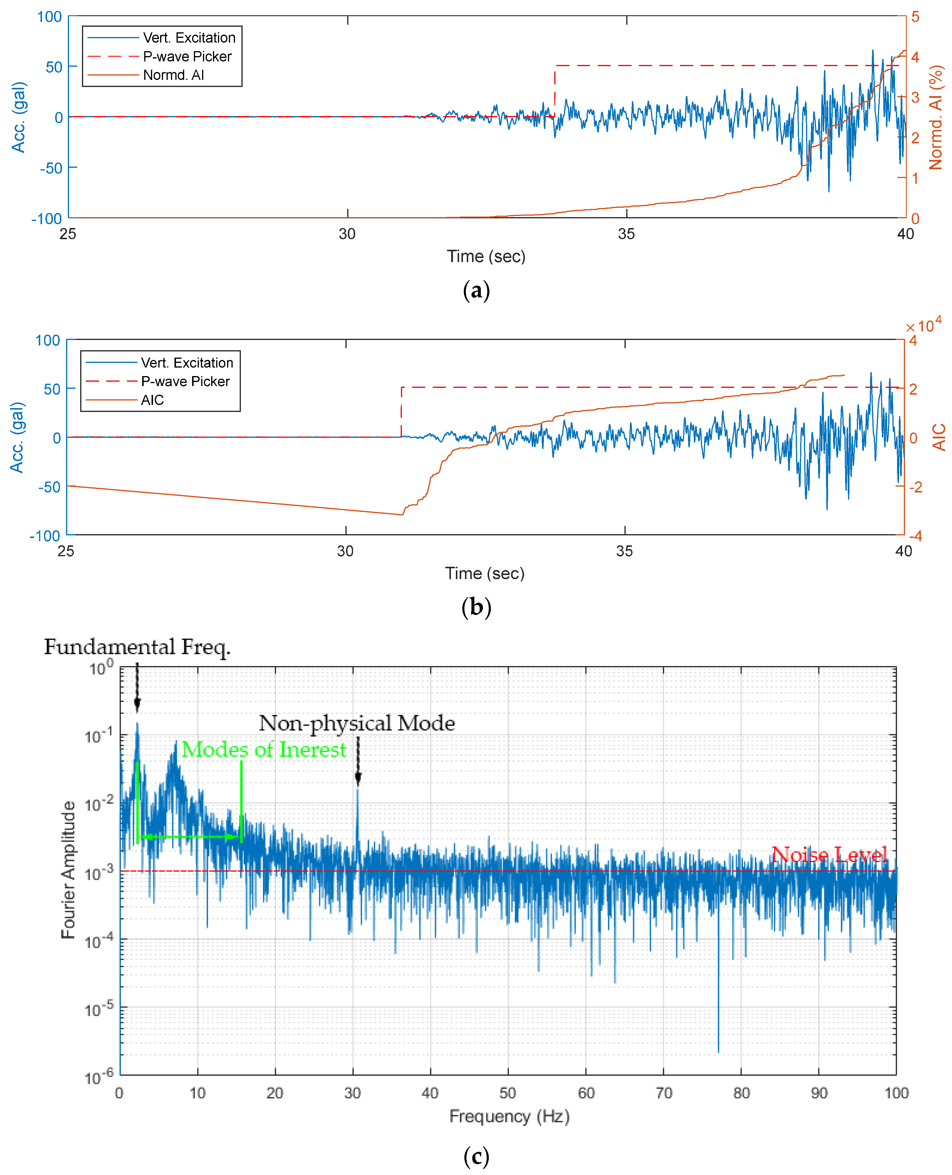
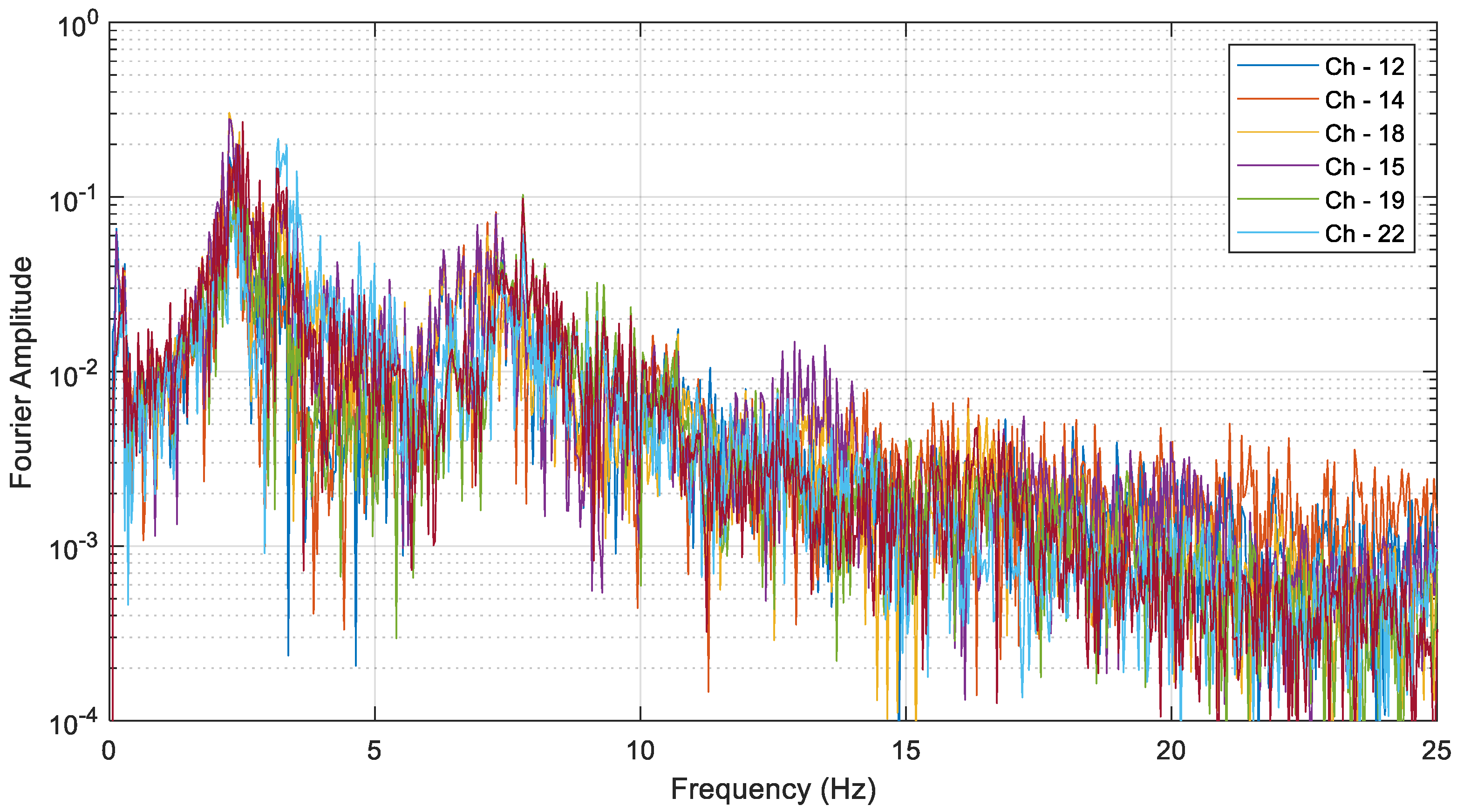
First, in the data preprocessing step, waveforms that were clearly distorted or exhibited dropouts or glitches were excluded from the measurements. The normalized Arias intensity and AIC were sequentially implemented to identify the arrival of P-waves, as well as to determine stationary excitations, as shown in Figure 2a. Then, FFT was applied to the acceleration responses with a 200 Hz sampling rate to provide an overview of the structure’s modal information, as shown in Figure 5. This example uses measurements collected on 21 September 1999 at 17:57:16 local time. It is worth noting that these measurements do not relate to the mainshock but rather the aftershock, by which point the seven-story RC frame had already undergone damage. After careful examination, the fundamental frequency of the seven-story RC building was about 3.2 Hz before the Chi-Chi earthquake and 2.3 Hz after the destructive earthquake. Moreover, the structure’s highest mode of interest was less than 20 Hz, so the acceleration responses can be down-sampled to 50 Hz—which corresponds to the Nyquist frequency of 25 Hz—to increase analysis efficiency.

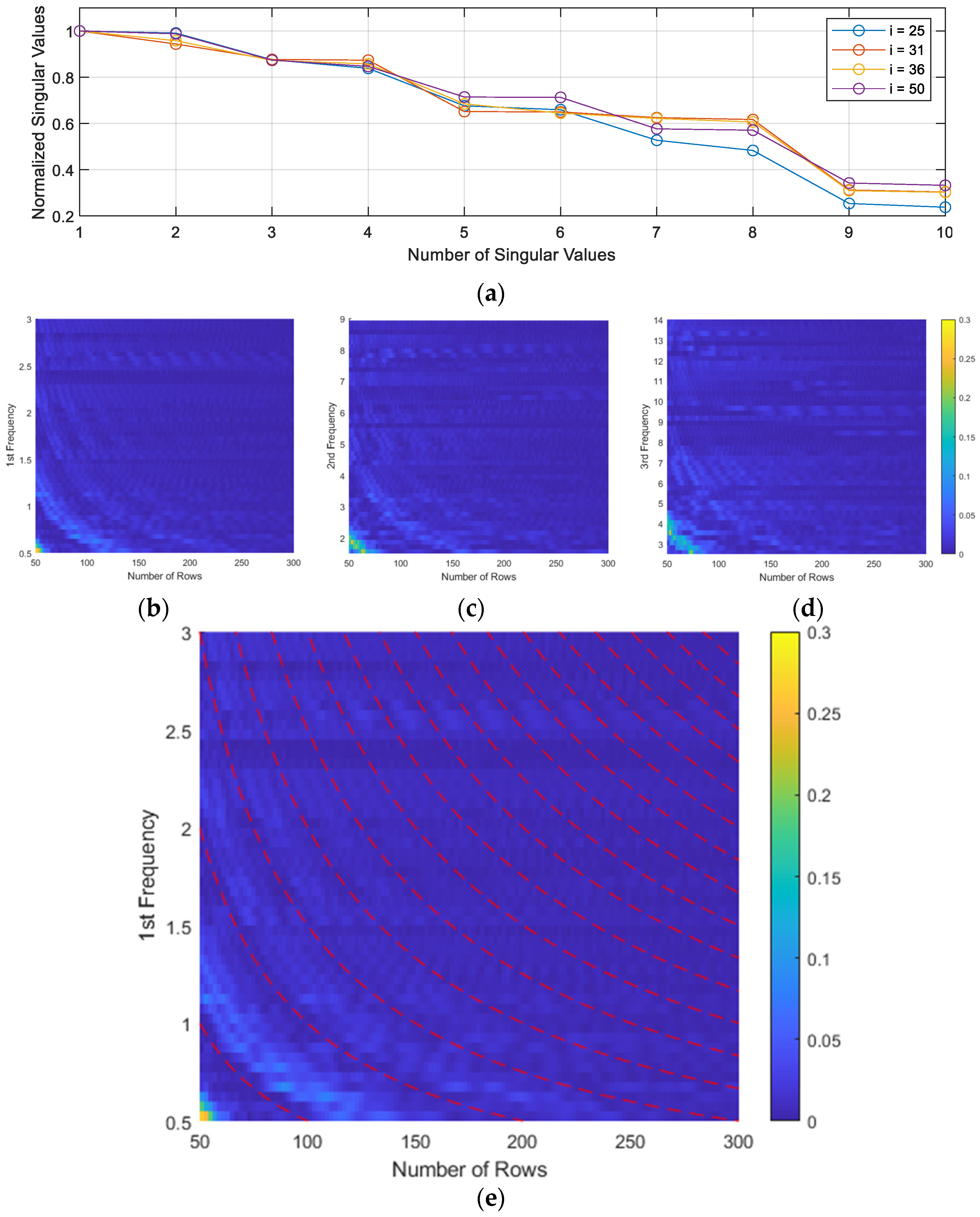
The next step is matrix construction and decomposition. According to Equation (14), the number of rows, i, can be selected as 8 (3.2 Hz) and 11 (2.3 Hz) and their multiples to secure the complete cycles of the lagged vectors for a clear decomposition. For example, Figure 6 shows the comparison of the normalized differences between the singular pairs with respect to different strategies. Clearly, the choice of the size of the Hankel matrix can affect the resultant decomposition performed by SVD, and the conventional method of selecting sequential numbers likely results in an incomplete decomposition, especially for the first mode, as shown in Figure 6a. Contrarily, the proposed procedure, according to the above-mentioned equation, can generate an elaborate isolation of every mode, providing well-separated singular pairs, as shown in Figure 6b.

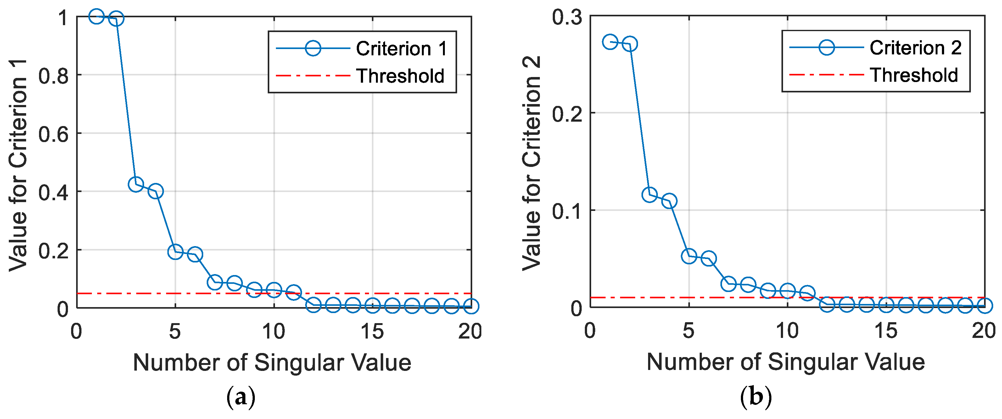
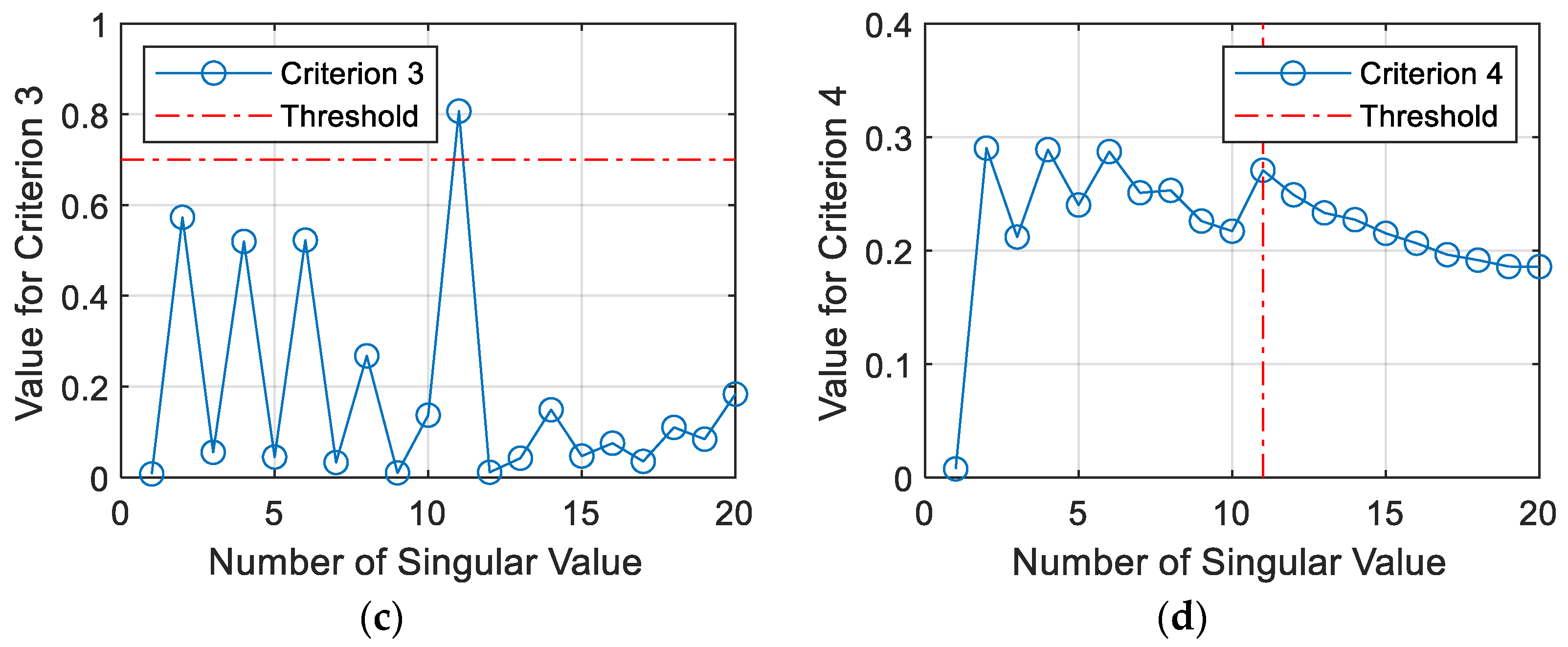
As stated in the previous section, the selection of system orders, n_e, is important when realizing the system in the final step. Figure 7 illustrates the results of the four approaches for estimating system orders through singular values. In this example, the size of the Hankel matrix is assigned as 22 to ensure differentiation of energy. Correspondingly, the criteria from C₁ to C₄, defined in Equation (15) to Equation (18), are 0.05, 0.01, 0.7, and 5, respectively, and the final selections of all approaches come to 11. The odd number resulting from the selection actually indicates that at least one spurious pole is extracted in the following system realization.

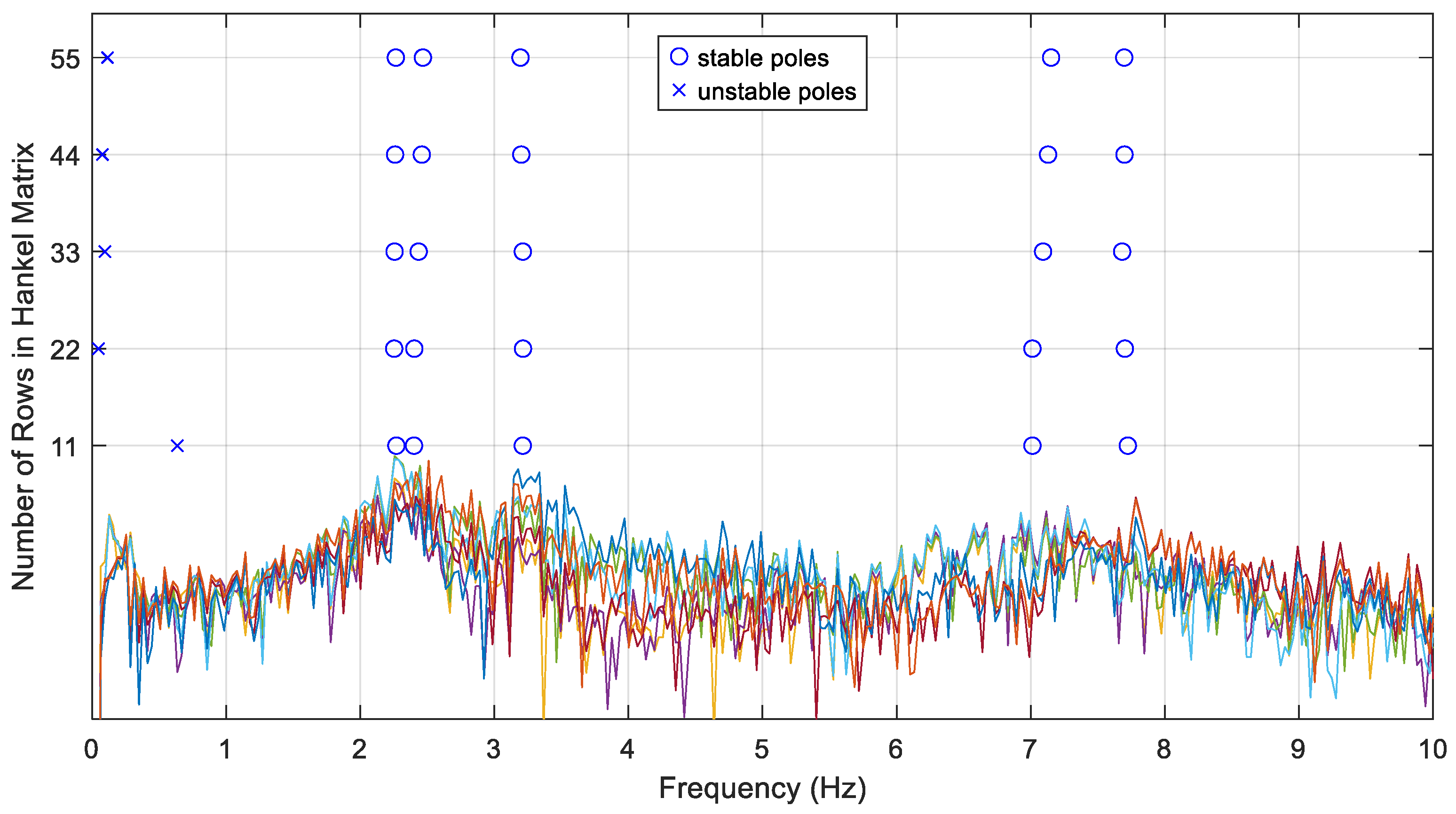
By assigning the system order as 11, Figure 8 depicts the stability diagram of the selected i together with the Fourier spectrum. Clearly, the identified frequencies are highly correlated with those observed in the Fourier spectrum. Five modes can be identified, including 2.27 Hz, 2.47 Hz, 3.19 Hz, 7.09 Hz, and 7.7 Hz. The consistency of the stability diagram also suggests that the proposed procedure provides clearer decomposition by designating the lagged vectors with complete cycles. The spurious mode can be further identified by applying the criterion of assured modes, which is represented as a cross in the stability diagram (unstable poles in Figure 8). This example generally illustrates the proposed three-step procedure for complex structures or field applications, and demonstrates the ability to produce reliable identification results.

Finally, the identified frequencies across the ten-year dataset are shown in Figure 9. It can be seen that the identification results with the proposed procedure are better than those without a carefully selected SSI matrix size and an adaptive estimation of system order, as shown in Figure 9a. With the proposed procedure, two more frequencies represent secondary modes, ranging from 5 Hz to 10 Hz, although some modes are not stimulated or identified in some measurements. Generally, this figure can be divided into three sections: the first seven sets of measurements represent the RC frame before the destructive earthquake, the eighth to thirteenth sets represent the frame after the earthquake, and the last three sets of measurements represent the last section, as separated by the red lines in the figure. According to the reconnaissance report by senior engineers, the destructive earthquake was identified as having caused moderate damage. The second section presents the damaged RC frame, which generates a 15% to 20% reduction in modal frequencies. Moreover, the report also indicated that the seven-story RC frame underwent repairs, representing the retrofitted RC frame, increasing the modal frequencies by about 5% to 10% in the results.

In the first two modal frequencies identified from the 16 sets of measurements, the average and the standard deviation of the overall error after applying the proposed procedure are around 1.99% and 1.89%, respectively. The error percentages range from 0.06% to 7.22%. On the other hand, the average and the standard deviation of the overall error before applying the proposed procedure are around 2.24% and 2.06%, respectively, while the error percentages range from 0.08% to 7.93%. Upon comparing these two cases, with and without a carefully selected SSI matrix size and an adaptive estimation of system order, it can be noted that the proposed procedure improved all the statistical indexes by approximately 10%. Most importantly, seven out of thirty-two modal frequencies are missed in the conventional SSI-based OMA; however, with the help of the proposed procedure, only two are missed, indicating three to four times superior performance in terms of identifying the structure’s mode in complex field applications.

4.4. Verification Result Using Four-Story RC Frame in Hualien

The second dataset includes 30 channels of accelerometers connected to the conventional SHM system, and it was collected from the RC building in Hualien, Taiwan. Figure 4b shows the sensor locations. Similar to the first dataset, only the structural responses in the longitudinal and transverse directions are exploited to identify the modal parameters, and the channels 4, 5, 10, 11, 13, 14, 16, 17, 18, 19, 22, and 23 are therefore used in the following verification. To discriminate nonstationary excitations, regarding the basic assumption, ground motions are measured through free-field sensors, although these channels are not shown in the figure. As a result, the structural responses from the ambient excitations, rather than the earthquake excitations, can be separated and analyzed by SSI.

Again, in the first step, waveforms that were clearly distorted or exhibited dropouts or glitches were excluded from the measurements. Then, the normalized Arias intensity and AIC were implemented to exclude nonstationary parts. FFT was applied to the acceleration responses before down-sampling, so that an overview of the structure’s modal information could be reviewed. Notably, this RC frame was also damaged by the Chi-Chi earthquake in 1999. After careful examination, the fundamental frequency of the four-story RC building was about 3.1 Hz before the Chi-Chi earthquake and 2.6 Hz after the destructive earthquake. Moreover, the structure’s highest mode of interest is less than 20 Hz, so acceleration responses can be down-sampled to 50 Hz—which corresponds to the Nyquist frequency of 25 Hz—to reduce the computational effect. Due to a high similarity with previous results and limited space, the results in the data preprocessing step are not demonstrated herein.

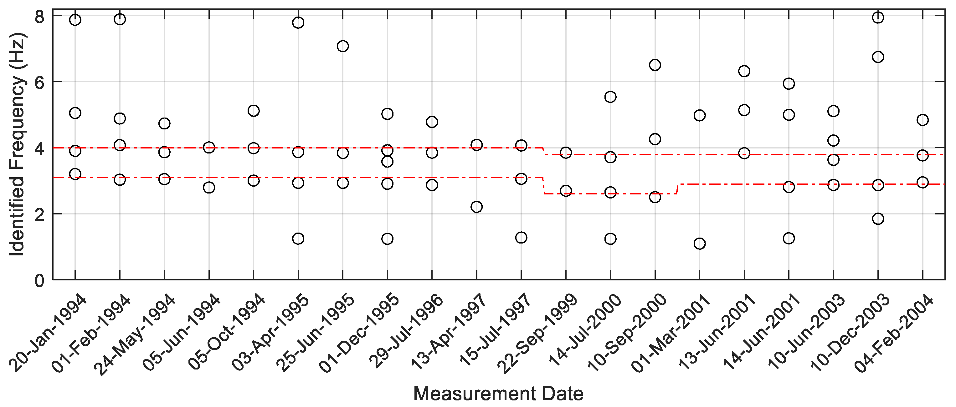
Figure 10 shows the identified frequencies across the ten-year dataset. Unfortunately, the results are more complicated than those in the first dataset due to several reasons, including smaller signals, stiffer behaviors, and more complex compartments. Some modes are not stimulated or identified in some measurements, such as the frequencies located at approximately 1.1~1.2 Hz, 5 Hz, and 8 Hz. Generally, two modes can be consistently observed from this figure, represented by the red lines in the figure. According to the reconnaissance report of the destructive earthquake, this frame was identified as having some damage by senior engineers, so an obvious drop can be found prior to 22 September 1999. The report also pointed out that the four-story RC frame underwent subsequent repairs around 2000. As a result, the fundamental frequency increased after 2001. The frame also underwent a further retrofit around 2010, in accordance with the nationwide school building enhancement program, although the measurements are not included in this dataset.

Lastly, the estimated system orders, using four approaches through singular values, are illustrated in Figure 11. From the first dataset, the proposed (fourth) approach shows more stable results over a decade, ranging from 8 to 18. In contrast, the first approach has the largest variation in both datasets because of its high dependency on the measured signals. The second approach seems more reliable compared to the first one; however, it kept advancing after the destructive earthquake and the structural repairs in the second dataset. This indicates that the second approach is difficult to update the results if the structural responses display increasing uncertainties. Typically, the third approach tends to underestimate the system order, although the estimated system orders are very similar to the proposed approach in the first dataset. The identified results may therefore lose many modes. Considering the identified frequencies in Figure 9 and Figure 10, the fourth approach is clearly the most highly recommended one.

4.5. Discussion on Limitations and Future Work Toward Full Automation

The effectiveness of implementing automated SSI-based OMA for long-term SHM has been investigated and illustrated using the aforementioned datasets. Consequently, the proposed procedure establishes a robust foundation for effective monitoring, facilitates early issue detection, and supports data-driven maintenance strategies. Certainly, it remains limited to assumptions regarding system identification based on SSI, as well as OMA, i.e., linear models, stationary excitations, and non-severe SNR, among other conditions. The identified modes are also restricted to the number and location of the sensors. For diagnosis and prognosis, experienced engineers are still preferred to carry out comprehensive assessment and provide informed decision-making concerning maintenance. However, applications of automated SSI-based OMA are not generally restricted by structure type, indicating a good transferability to other structure types or domains once the measurement configuration is adequate. When building a fully-automated SHM system, the P-wave picker can be abridged if stationary excitation can be secured. Moreover, further study is also recommended to fully demonstrate the continuous performance of SHM systems before field deployment, in particular, a detailed investigation on damage detection.

5. Conclusions

The accurate identification of modal parameters is essential for SHM, and this can be achieved by exploiting the structural responses measured in ambient environments following the OMA framework. Considering its versatility in handling real-world structural monitoring challenges, SSI is particularly applicable to complex structures or field applications. This study aims to propose a three-step procedure for implementing automated SSI-based OMA, including data preprocessing, matrix construction and decomposition, and system realization. To verify the effectiveness of the proposed procedure, two datasets, collected using conventional SHM systems, were investigated and analyzed herein. Accordingly, it is evident that the selected size of the SSI matrix, the estimation of system order, and the removal of spurious modes can significantly enhance system identification techniques, providing a 10% improvement in overall error rates. Most importantly, loss rates, in identifying structure mode in complex field applications, can be decreased by approximately three to four times, and therefore, continuous and long-term SHM can be facilitated by enhanced SSI, implemented with the proposed three-step procedure. The conclusions drawn from these results can be summarized as follows:

• The techniques of P-wave pickers can be utilized to differentiate nonstationary excitation and secure analysis based on OMA and SSI.
• The preliminary identification of fundamental frequency helps the overall automated work through down-sampling, sizing the Hankel matrix, and clarifying the stability diagram.
• Assigning the size of the Hankel matrix with integers multiplied from the fundamental periods can improve decomposition with lower differences between pairs and avoid spurious modes.
• The proposed decay function provides a good estimation of system order by finding the first point at which the system experiences a steady descent.
• The proposed three-step procedure based on SSI can facilitate automated OMA for continuous and long-term SHM, in terms of adjusting user-defined parameters autonomously.

Identifying modal parameters accurately is crucial for complex and field-based SHM systems, as it establishes a robust foundation for effective monitoring, facilitates early issue detection, and supports data-driven maintenance strategies. Moreover, diagnosis and prognosis grounded in a thorough physical understanding of structural behavior offer valuable insights for comprehensive assessment and informed decision-making regarding maintenance. Although this study has provided initial validations, further research is recommended—particularly a detailed case study on damage detection—to more fully demonstrate the continuous performance of SHM systems prior to field deployment.