1. Introduction
Fuzzy logic methods emerged in the mid-1960s with the foundational work presented in [
1], where a fuzzy set is defined through a membership function that assigns each element a degree of membership ranging from zero to one. Subsequently, in 1973, Zadeh expanded on this concept by introducing fuzzy algorithms, which are structured sequences of instructions formulated through IF-THEN rules [
2]. In the same year, the first documented industrial application of fuzzy logic was reported in [
3]. This study explored the development of a “linguistic” controller for a steam engine model, aiming to analyze human interaction with adaptive control strategies. Unexpectedly, the fuzzy control approach demonstrated superior performance, significantly exceeding expectations and fostering broader interest in the application and advancement of fuzzy logic systems
The work presented in [
4] compares fuzzy control methods with other nonlinear control strategies. It points out that a major drawback of fuzzy control lies in its inability to clearly define a direct link between membership functions and the system’s states, an unresolved issue. The authors also suggest that nonlinear control approaches, especially those specifically adapted to the system’s structure, often demonstrate superior performance compared to fuzzy techniques. The study presented in [
5] focuses on Takagi–Sugeno–Kang (TSK) fuzzy systems, which enable the representation of general nonlinear dynamics through a compact set of rules. This work also introduces a methodology for designing fuzzy controllers capable of ensuring closed-loop stability when using TSK models. A practical implementation of fuzzy control is illustrated in [
6], where a fuzzy logic controller is applied to a magnetic levitation system of a metallic sphere. The main contribution lies in the comparative analysis between the fuzzy controller and both linear (PD and PID) and nonlinear alternatives. The results reveal a superior performance of the fuzzy controller, primarily due to its effectiveness in managing the inherent nonlinearities of the system.
The research outlined in [
7] introduces the well-established Takagi–Sugeno (T–S) identification method for modeling systems based on input–output data. A notable limitation of this method is its inapplicability in scenarios where membership functions exhibit pairwise overlap. To address this shortcoming, the approaches proposed in [
8,
9] incorporate parameter weighting to refine the values obtained through standard T–S identification, thereby mitigating the constraints of the original formulation. Furthermore, a Linear Quadratic Regulator (LQR) is employed to evaluate the performance of the proposed estimation framework. Validation through two illustrative examples confirms the robustness, simplicity, and general applicability of the algorithm developed.
The study conducted in [
10] illustrates the application of modern control theory, rooted in time-domain analysis and state-space modeling, to systems with multiple inputs and outputs, including those exhibiting nonlinear behavior. In this study, the authors address the challenges posed by complex airflow dynamics, noting that few models adequately capture the dynamic distribution of indoor temperature. To improve accuracy in temperature prediction and control, a state-space model is employed and experimentally validated, yielding realistic and reliable results. Similarly, the study in [
11] proposes an enhanced aeroservoelastic modeling framework for gust load analysis using time-domain state-space representations. The approach effectively handles the computational complexity of gust calculations and proves advantageous for control system design. A subsystem realization methodology is introduced to construct the full aeroservoelastic model, with simulation results confirming its high predictive accuracy.
The contributions presented in [
12,
13] demonstrate further applications of the state-space modeling paradigm in control design. Di Ruscio [
12] incorporates the model within a model predictive control framework, whereas [
13] utilizes it for the regulation of a four-tank process. In the latter study, as is common in system identification tasks, the derivation of accurate models typically requires full knowledge of both input and output signals. However, when one or more inputs are partially unknown, the identification process becomes significantly more challenging or even infeasible. To address this limitation, the methodology proposed in [
14] introduces an iterative estimation procedure capable of reconstructing the system state trajectory and inferring the unknown input signal based solely on output measurements. This technique effectively mitigates one of the primary obstacles associated with conventional identification approaches.
The control strategy outlined in [
15] leverages the incremental state-space model to achieve zero steady-state error in response to step-type reference signals. This formulation is further employed in [
16] for the optimal multivariable control of a wind turbine system. The evaluation involves the application of Linear Quadratic Regulator (LQR) controllers to a nonlinear wind turbine model, with simulation results indicating favorable transient performance and complete steady-state error rejection, even in the presence of external disturbances, nonlinearities, and model inaccuracies. The work in [
17] reinforces the suitability of the incremental modeling approach for addressing the intrinsic nonlinearity and uncertainty of the plant. Additional findings in [
18] demonstrate that incremental control strategies can effectively resolve continuous-time nonlinear control problems without requiring a comprehensive global model of the system.
The foundational work in [
19] demonstrates that the state vector of a linear system can be reconstructed by monitoring the system’s inputs and outputs. This study introduces the concept of a state observer, which enables estimation of the system’s internal states when direct measurement is impractical—a common scenario in real-world control applications. The relevance of this methodology is further substantiated in [
20,
21], where state observers are employed to estimate the system states and facilitate the design of optimal state-feedback controllers. Simulation analyses presented in both references validate the proposed approaches, highlighting their ability to ensure global stability and accurate state estimation.
The comparative study conducted in [
22] analyzes the performance of three advanced state observers: high-gain, sliding mode, and extended state observers developed to address the inherent limitations of classical observer designs. The results indicate that the extended state observer outperforms the others in terms of robustness to dynamic uncertainties, sensor noise, and external disturbances. A similar evaluation is presented in [
23], where the Luenberger estimator, Kalman filter, and sliding mode observer are assessed for estimating the speed of a DC motor. The findings underscore that observer performance is highly dependent on the specific characteristics of the system, with each method exhibiting distinct advantages under different operational conditions.
The Linear Quadratic Regulator (LQR) has been widely adopted in state-space control for both continuous- and discrete-time systems due to its inherent robustness and optimal performance characteristics. Wong [
24] employs the LQR to demonstrate its ability to ensure system stability under predefined conditions, even in the presence of actuator faults and significant external disturbances. A complementary study is presented in [
25], where the LQR is integrated into a fuzzy control architecture. In this case, the nonlinear system is linearized using the Lyapunov linearization technique and modeled through the Takagi–Sugeno (T–S) fuzzy framework. This representation enables the implementation of an LQR controller within each locally linearized region. The simulation results confirm that the combined approach yields quasi-optimal system performance, underscoring the effectiveness of embedding LQR within fuzzy modeling structures.
The investigation performed in [
26] presents a comparative evaluation of the Linear Quadratic Regulator (LQR) and the Proportional-Derivative (PD) controller, applied to the attitude control of a quadrotor, a system characterized by nonlinear dynamics. MATLAB 2014 based simulations are employed to assess key performance indicators, including settling time and overshoot percentage. The results indicate that the LQR, despite being a linear control strategy, is capable of delivering satisfactory performance in controlling the nonlinear system, thus validating its applicability in such contexts.
The work presented in [
27] introduces an enhancement to the Linear Quadratic Regulator (LQR) through the inclusion of an integral feedback component aimed at improving steady-state accuracy. This modification achieves a notable reduction in steady-state error—from over 40 cm to less than 1 cm—demonstrating the effectiveness of integral action as an extension to the LQR for applications demanding high precision. A comparable methodology is explored in [
28], where an optimal control scheme based on the LQR is designed for the position and attitude regulation of a quadcopter UAV. In this case, integral compensation is selectively implemented for vertical position control. The simulation outcomes confirm that the proposed control structure successfully eliminates steady-state error in altitude regulation.
The methodology applied in [
29] presents a comparative evaluation of a state feedback controller (SFC), designed using a linearized model and a Linear Quadratic Regulator (LQR), against a conventional PID controller. The findings indicate that, with appropriate parameter tuning, the SFC markedly improves the dynamic performance of the system. Specifically, it achieves a reduction in steady-state error and delivers an enhanced transient response, thereby offering a more robust control solution compared to the traditional PID approach.
Extremum Seeking Control (ESC), initially introduced in [
30], constitutes an adaptive control strategy that enables a system to converge toward the optimum of a measured performance index without requiring a priori knowledge of the plant model. The method operates by iteratively minimizing a cost function through the adjustment of specific optimization parameters. A significant resurgence of interest in ESC was driven by the contribution in [
31], where a formal proof of convergence was established for the standard ESC scheme utilizing periodic perturbations in the context of nonlinear systems.
The application of Extremum Seeking Control (ESC) for PID tuning is explored in [
32], where ESC is utilized to minimize a cost function and, thereby, identify the optimal parameters of a PID controller. The comparative analysis reveals that ESC achieves superior performance—specifically, a reduced settling time—relative to traditional tuning techniques such as Ziegler–Nichols (ZN), Internal Model Control (IMC), and Iterative Feedback Tuning (IFT). A related contribution is presented in [
33], which proposes a novel PI controller design method grounded in ESC principles. This approach is formulated to address real-time optimization tasks, thereby illustrating the adaptability of ESC for dynamic control environments.
As discussed in [
34], enhancing process performance typically involves the application of real-time optimization (RTO) or model-based control techniques. Although these strategies can be effective, they often entail considerable computational overhead, and model-based controllers are notably susceptible to disturbances not accounted for in the model. In contrast, Extremum Seeking Control (ESC) offers a model-free alternative that circumvents these issues but is constrained by slow convergence rates. To address this limitation, the integration of automatic optimization control is proposed as a means to reduce computational complexity. The case study involving an ammonia reactor illustrates that the combined use of ESC and automatic optimization enables effective compensation for unmeasured disturbances and plant-model discrepancies, thus improving overall system robustness.
The methodology presented in this work aims to ensure zero steady-state error in response to various reference and disturbance signals, including step, ramp, and second-order polynomial (parabolic) inputs. The proposed control scheme combines the incremental state and incremental-N state modeling frameworks with the Takagi–Sugeno (T–S) fuzzy representation to address nonlinear system dynamics. To improve the controller tuning process, Extremum Seeking Control (ESC) is integrated into the design. The effectiveness of the approach is validated through a case study involving a thermal tank system, selected due to its inherent nonlinear behavior and multivariable characteristics.
The structure of the paper is as follows:
Section 2,
Section 3 and
Section 4 introduce the incremental state-space model, its fuzzy extension via Takagi–Sugeno rules, and a nonlinear parameter identification method.
Section 5 and
Section 6 address discrete LQR control and state estimation.
Section 7 and
Section 8 detail the construction of incremental-2 and generalized incremental-N models, including their fuzzy formulations.
Section 9 presents the Extremum Seeking Control (ESC) algorithm for automatic LQR tuning.
Section 10 applies the proposed fuzzy control strategy to a nonlinear thermal mixing tank, evaluating its performance and robustness across various reference signals and disturbance scenarios.
7. Incremental-2 State Model
As seen in
Section 2, it is straightforward to obtain the incremental state model using Equation (
11). For this reason, the question arises as to what would happen if this equation were applied again to previously calculated incremental state matrices. By doing so, a new state model is obtained, which we will refer to as the incremental-2 state model. This model naturally allows for the introduction of a second integrator into the control algorithm. If we apply the process described by Equation (
11) to the previously obtained incremental model, namely, Equation (
13), we obtain the following:
where
,
y
. In matrix form, it would be
where
,
and
, thus obtaining the new extended vector of incremental-2 state,
:
The feedback matrix of the incremental-2 state can be designed using the discrete LQR method, which requires for its calculation the state matrices
and
, as well as the matrices
y
. Following the process described in
Section 3, and since the objective of the control is to achieve a steady-state output
, the extended reference state of the incremental-2 model would be defined as
and the controller is described as follows:
where
,
,
and
, and the control action is
If the feedback system is stable and steady state is approached, the following is true:
and, thus,
So, if
and
are of rank
q, it is verified that
Therefore, the controlled system has a steady-state error equal to zero in response to step-type inputs and disturbances, and even to ramp-type inputs. It is important to highlight that the control action (
40) has been calculated in an incremental-2 form, which is equivalent to applying a double integral control action. Similarly to the incremental model, for the incremental-2 model, it is necessary to use a state observer, since
is not accessible. Based on Equation (
27), the incremental-2 state can be estimated as follows:
With Equations (
41) and (
28), the observer can be described as
where
is calculated in the same way as in Equation (
31).Thus, the observer of the extended vector of the incremental-2 state would be
8. Fuzzy Incremental-N State Model
An iterative algorithm has been proposed to obtain an incremental-N state model that introduces N integrators and can achieve zero steady-state error in response to polynomial-type inputs and disturbances of order N-1. To do this, the extended state matrices are initialized by assigning them to the traditional discrete-state matrices:
Using a loop, the extended state matrices are recalculated N times:
In this way, the incremental-N state model would be defined:
In matrix form,
where
,
, and
, thus obtaining the new extended vector of incremental-N state,
. This would be
and the reference state is
The controller and control action for the incremental-N would be defined:
where the incremental-N state feedback matrix K can be obtained, for example, using the discrete LQR method, whose calculation will use the state matrices
and
obtained through the recursive algorithm of Equation (
45), along with the matrices
and
. For the incremental-N model, as with the previous incremental models, a state observer is required since
is not accessible. Following the approach of Equations (
27) and (
41), we can estimate the incremental-N state as follows:
Following the approach of the Equations (
42) and (
51), the observer can be described as
where
is calculated in the same way as in the Equation (
31). Thus, the observer of the extended incremental-N state vector is defined:
Since the goal is to achieve fuzzy control using the incremental-N state model, the method to be used is explained below. First, after completing the linear identification and T–S identification, the nonlinear system is modeled using the incremental-N T–S state model. Starting from Equation (
46), we obtain
From this, we can express its matrix form using the T–S fuzzy model, taking Equation (
47) as a reference:
where
,
and
, and they are calculated using the iterative method presented in Equations (
44) and (
45). Then, a discrete LQR controller is used, the calculation of which will use the state matrices
and
, as well as the matrices
and
. For this reason, to obtain the controller and the control action, we start from Equation (
50), to which the T–S fuzzy model is applied. In this way, the following is obtained:
Finally, a fuzzy state observer is used because the state
is not accessible. This observer is obtained by applying the T–S fuzzy model to Equation (
52):
where
is calculated using the Equation (
34).
10. Thermal Mixing Tank System
In this section, the application of fuzzy control based on the incremental-N state model is illustrated through the thermal mixing tank case study [
15,
35,
36]. The purpose is to evaluate the system’s performance and verify the achievement of zero steady-state error in response to step, ramp, and subsequent input and disturbance signals. The thermal mixing tank system, depicted in (
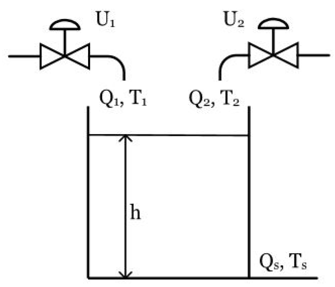
Figure 1), is a multivariable and nonlinear system comprising a tank, two inlet valves (for hot and cold fluids), and an outlet pipe. The primary control objective is to regulate the outlet flow rate
and the outlet temperature
to their respective setpoints, under the assumption that the outlet temperature is equal to the temperature within the tank.
The system inputs are two valves: One transports a hot fluid at a constant temperature
with a variable flow rate
, and the other transports a cold fluid at a constant temperature
with a variable flow rate
. Both flow rates serve as the manipulated variables of the system, controlled through their respective motorized valves, whose dynamic model is given by
Additionally, it is assumed that there are heat losses proportional to the temperature difference between the interior
and the exterior
of the tank, which act as a disturbance to the system. Thus, the dynamic model is given by
Substituting (
64) into (
62),
And substituting (
62) into (
66),
The model can also be expressed in function of
, starting from (
64):
Thus, the complete model would be
where the parameters of the thermal mixing tank system are shown in
Table 1. Similarly,
Table 2 describes the values of the nominal operating point of the system. In (
69), it can be seen that
is of order 2 and that
is of order 3.
The open-loop simulation of the system was carried out using the Simulink tool from Matlab, with a sampling time of 0.5 s and a total simulation time of 50,000 s. The effect of actuator saturation was explicitly addressed in the simulation framework by constraining the control inputs during the design phase. Specifically, the maximum flow rate for each actuator was limited to 4 (m
3/s). Once the system data were obtained, a linear identification was performed using the classical least squares method to estimate an initial set of parameters
for both the outlet flow rate and the outlet temperature. This identification process is as follows:
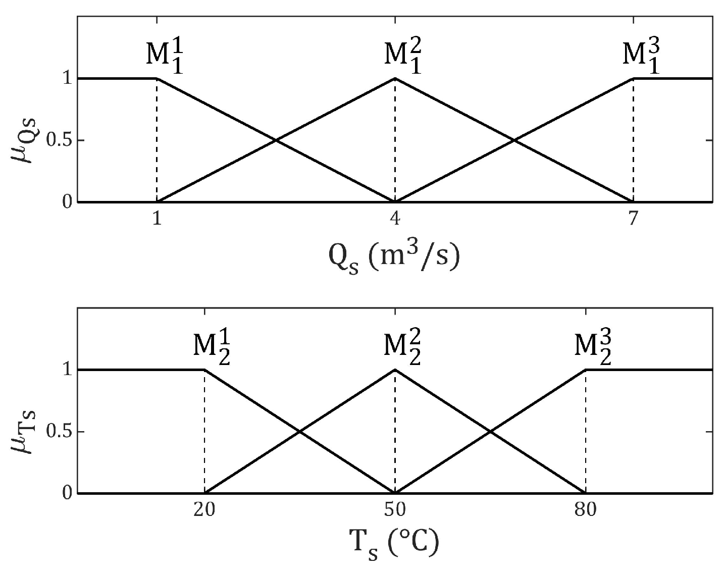
The next step is to apply the identification of the T–S fuzzy model. To this end, three fuzzy sets are selected between 1 and 7 (m
3/s) for the flow rate, and another three between 20 and 80 (°C) for the temperature. Both membership functions are shown in
Figure 2.
In this way, the fuzzy model is constructed using a set of 9 rules:
The next step is to model the nonlinear system using the incremental state T–S model. This is achieved by applying Equation (
15) presented in
Section 3:
where
,
, …,
,
and
C are calculated using Equations (
2)–(
4). So,
In the same way, the matrix notation of the T–S incremental state model is obtained using Equation (
16), thus obtaining
where:
Once the model is obtained, the feedback matrix
K for all the fuzzy rules. To do this, the matrices
Q and
R are used, which are defined as follows:
And so, the controller for each fuzzy rule is defined as
Finally, remembering that the state
, we must calculate the matrix
H of the state observer for each fuzzy rule using Equation (
34) of
Section 6:
Based on the results obtained, a fuzzy controller using the incremental state model was successfully implemented for the thermal mixing tank system. To evaluate the performance of the fuzzy controller on the nonlinear system, changes were applied to the reference inputs of
and
, as well as disturbances affecting both variables.
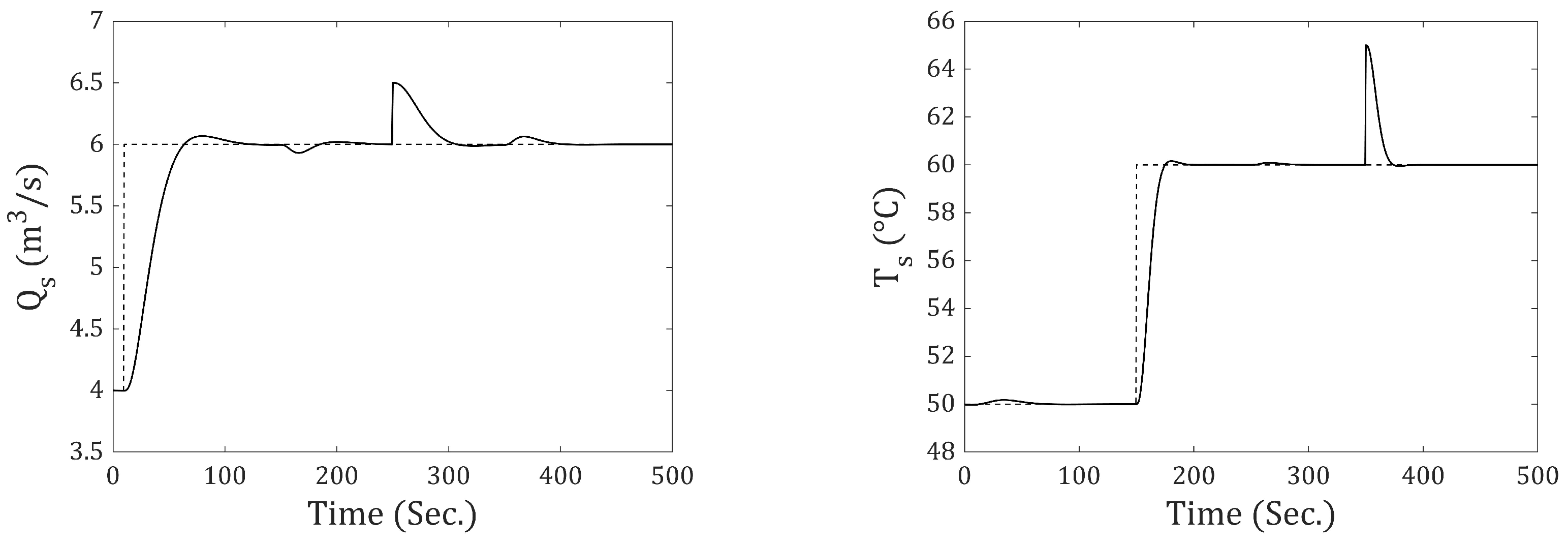
Figure 3 show the responses of
and
to step changes: One step input is applied to
at 10 s and another to
at 150 s, along with step-type disturbances. The disturbance affecting
occurs at 250 s with an amplitude of
(m
3⁄s), while the disturbance affecting
occurs at 350 s with an amplitude of 5 (°C). Moreover, in
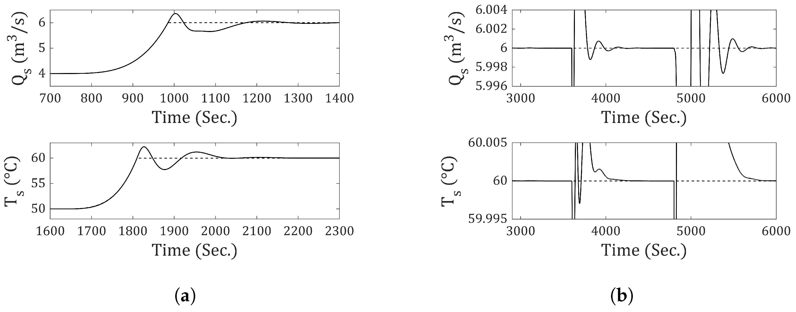
Figure 4, it can be observed that the system can withstand excessive changes in the reference input, which confirms its correct operation even in regions far from its nominal operating point.
It can be observed that a zero steady-state error has been achieved in response to step-type inputs and disturbances for a nonlinear system using a fuzzy control based on the incremental state model. However, the
Q and
R values are not optimal; in other words, a better response can still be obtained. A clear example would be to make the system faster while ensuring that the overshoot peaks are not excessively high. To obtain these optimal values, the ESC (Extremum Seeking Control) explained in
Section 9 is used, which aims to minimize the cost function shown in Equation (
58), corresponding to the MSE (Mean Squared Error).
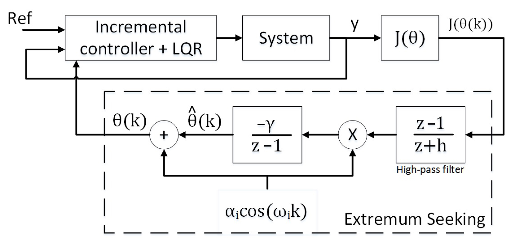
As illustrated in the
Figure 5, the ESC algorithm iteratively updates the controller parameters
based on the current value of the cost function
. At each iteration, the algorithm evaluates
using the updated parameters and subsequently adjusts
to minimize the cost. This procedure is repeated until convergence is achieved, i.e., when
reaches a local minimum, thereby yielding an optimal parameter configuration.
This optimization is achieved by periodically perturbing the system, usually using a sinusoidal wave, and then estimating the gradient . The gradient is computed by first filtering the discrete-time signal using a high-pass filter to remove the DC component. Next, the signal is demodulated by multiplying it with a discrete sinusoidal wave of the same frequency as the perturbation signal. Finally, the result is integrated using a step size to obtain a new estimate of the parameter . It is worth noting that the integrator acts as a low-pass filter.
For the case of the thermal mixing tank system, the following cost function will be used:
where
and the scaling factor 0.01 is introduced to ensure that the output flow rate error
and the output temperature error
contribute comparably to the cost function. In general, the magnitude of the temperature signal is approximately 10 times larger than that of the flow rate. As the cost function involves squared errors, this discrepancy is further amplified—potentially causing the temperature error to contribute up to 100 times more than the flow rate error. To address this imbalance, a weight of 0.01 is applied to the temperature term, effectively normalizing both error contributions to a similar scale. Therefore, the chosen scaling factor is not arbitrary; it ensures that both variables influence the optimization criterion in a balanced manner, despite their differing physical units and dynamic ranges. Once the cost function is defined, the initial values for the
Q and
R matrices are selected:
The value of 0.001 was chosen through iterative testing because if it were larger, it caused failures in the controller; on the other hand, if it was too small, a good response was not obtained. Since
R is the weighting matrix for the control action of the system and its variables have the same weight,
will change in the same way as
. Similarly, for the
Q matrix, only the values of
,
and
are varied, since multiple simulations have shown that variations in the remaining terms do not significantly affect the performance of the control system. In fact, it has been verified that the values from
to
can be set identically without degrading control quality. Thus, the configuration is as follows:
This simplifies the simulation run time and makes it less complicated to select appropriate values for
,
and
. It should be noted that
and
influence the stability and convergence of the method, and that
where
. The optimizer values are obtained through an iterative search to ensure that the method is stable and able to converge. These values are
where a value of
was chosen to calculate
. It can also be seen that
, since it is intended to keep
so that their values remain unchanged throughout the entire iteration. This serves as a reference and allows the focus to be placed solely on the
Q matrix. It is worth noting that it has been verified that the optimization is not affected if the value of
remains constant.
Since the goal is to obtain the values that optimize the cost function, it is recommended to apply ESC globally. That is, the system should be subjected to large variations in the reference input for both output flow rate and output temperature across its entire operating range.
Table 3 shows the selected points, establishing the path from point 1 to point 11 and then returning back to point 1.
Figure 6 shows the convergence of
and the values obtained for the
Q matrix. It can be observed that the value of
continues to increase; however, the value obtained at iteration number 500 is taken, since
no longer decreases. The resulting
Q and
R values are as follows:
The feedback matrix
K is obtained for each fuzzy rule, which is defined as
Figure 7 and
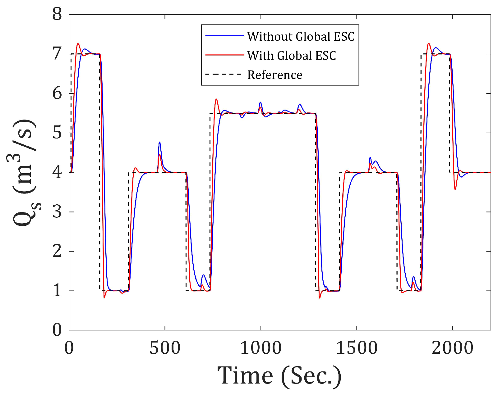
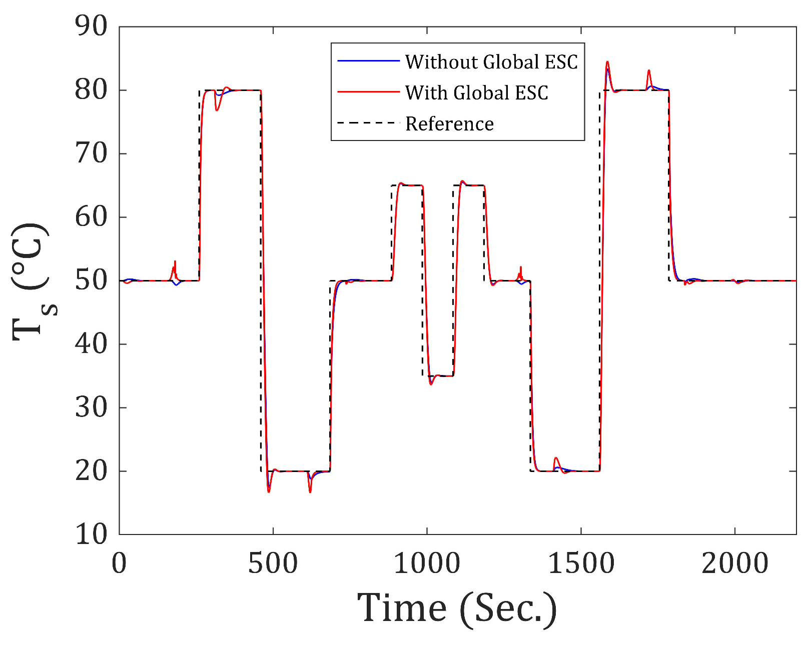
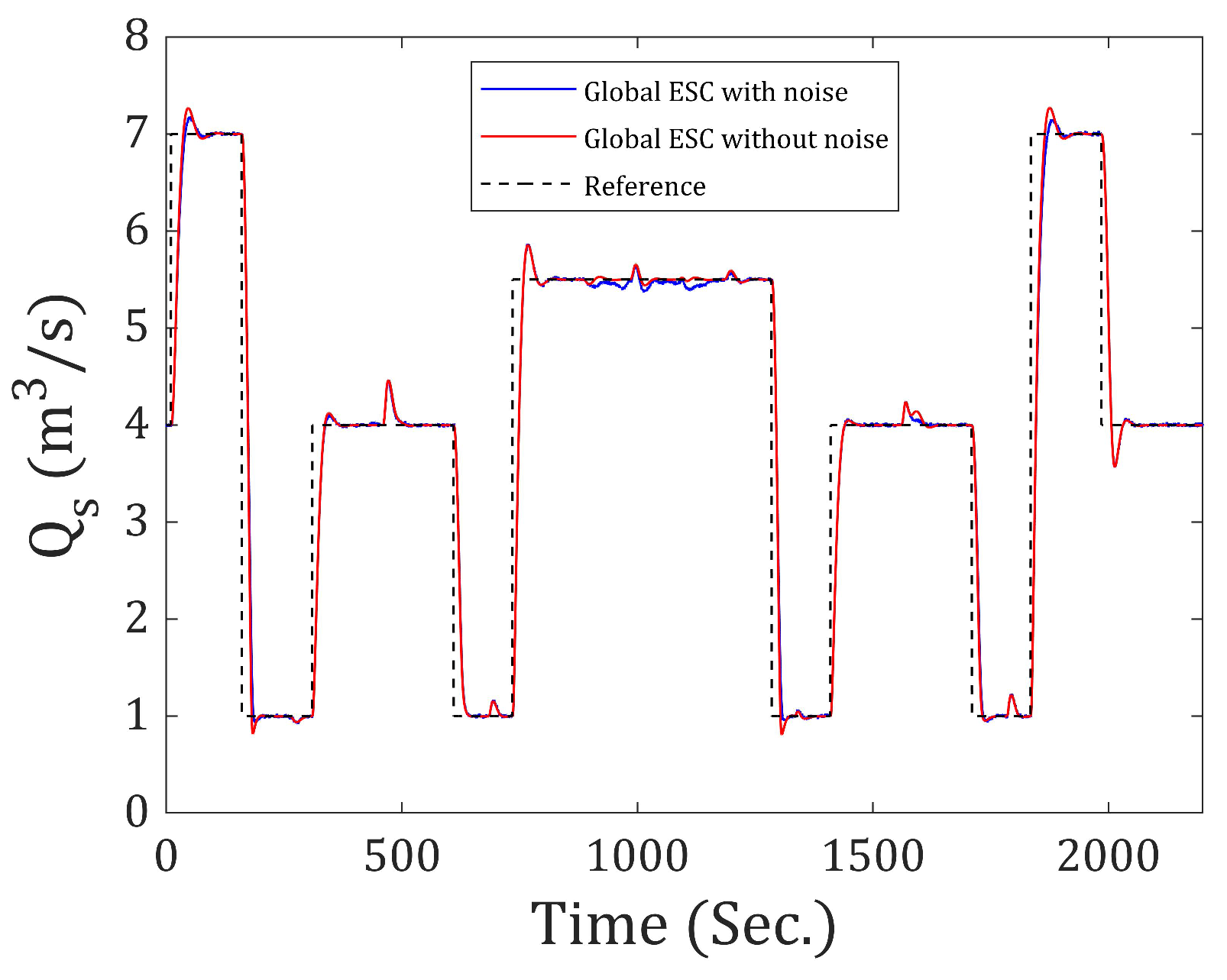
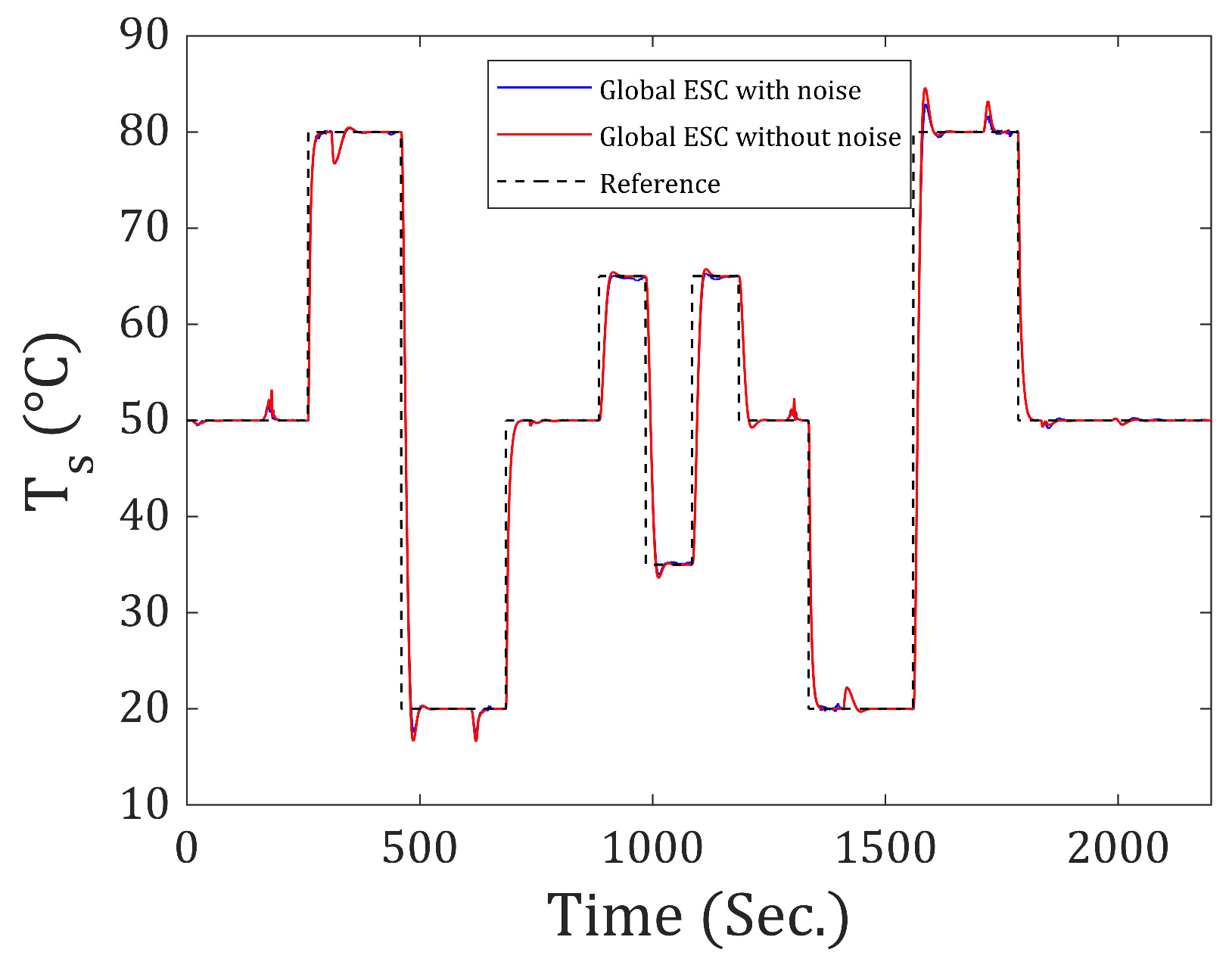
Figure 8 show the responses of flow rate and output temperature to excessive step-type input throughout the operating range of the nonlinear system, comparing the system when ESC is not used with the values obtained for the matrices
Q and
R using Global ESC.
As shown in
Figure 7, by using Global ESC, a better response is obtained in the output flow rate. It is faster and exhibits a smaller amplitude in the peaks that occur when there is an abrupt temperature change and the flow rate remains constant. On the other hand, in
Figure 8, it can be seen that using ESC slightly increases the peaks in the temperature response when it remains constant and the system is subjected to an abrupt change in the flow rate. However, a faster response is achieved. This can be better understood by looking at
Table 4, which shows the cost function
and the RMSE (Root Mean Square Error) value for
and
, comparing the method used to obtain the matrices
Q and
R.
This confirms that the application of ESC leads to an improved and faster response under excessive step inputs. Moreover, this method simplifies the determination of the optimal values for the matrices Q and R.
11. Responses for the Incremental-N
In a similar manner, this procedure can be applied to the incremental-N approach in order to analyze the system’s behavior at each incremental stage under reference changes and output disturbances, as well as input disturbances and measurement noise.
11.1. Step-Type Reference and Output Disturbance
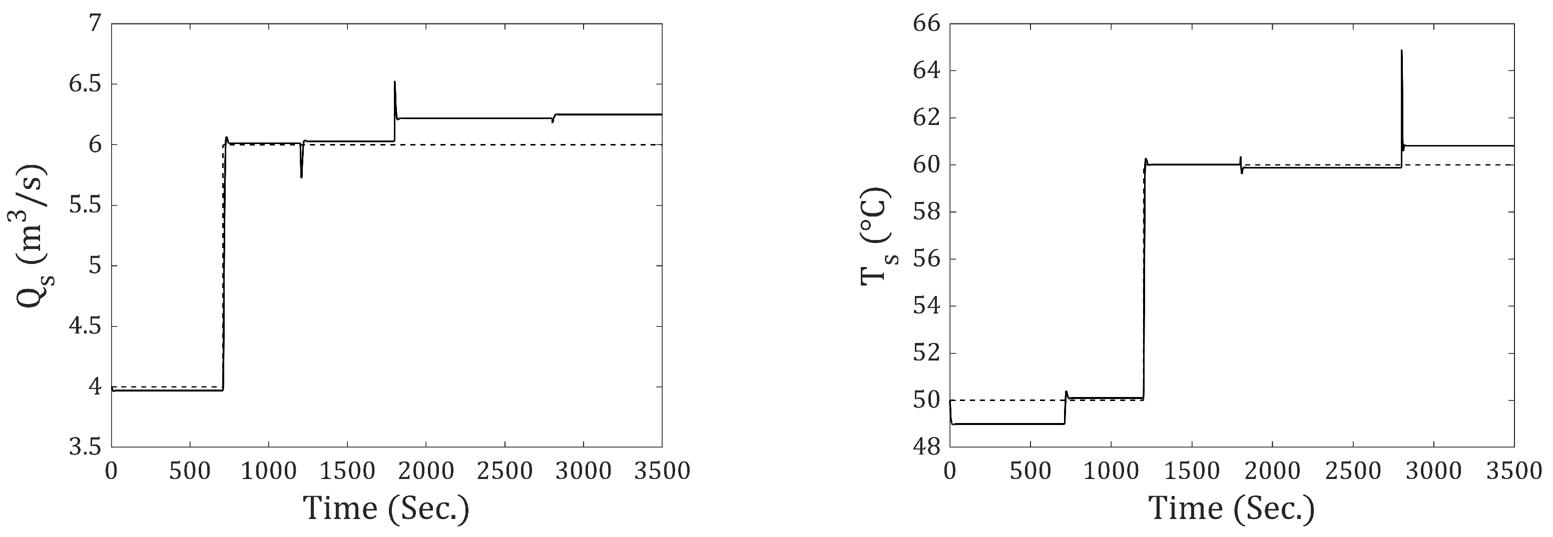
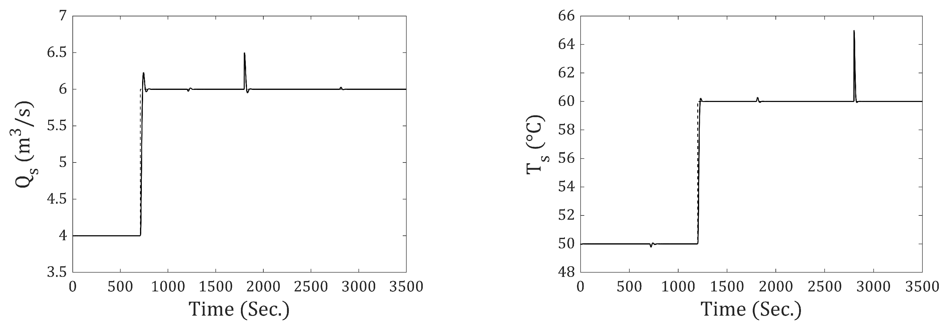
The results are presented for the system subjected to step-type reference and disturbance inputs. A simulation time of 3500 s was used for all cases. The step input for the output flow rate () occurs at 710 s, and for the output temperature (), it occurs at 1200 s. The disturbance for has an amplitude of (m3⁄s) and occurs at 1800 s. For , the disturbance has an amplitude of 5 (°C) and occurs at 2800 s.
Figure 9 presents the output flow rate and temperature responses using the traditional discrete-state model (incremental-0). In both cases, it can be seen that the system fails to achieve zero steady-state error. From
Figure 10,
Figure 11,
Figure 12,
Figure 13 and
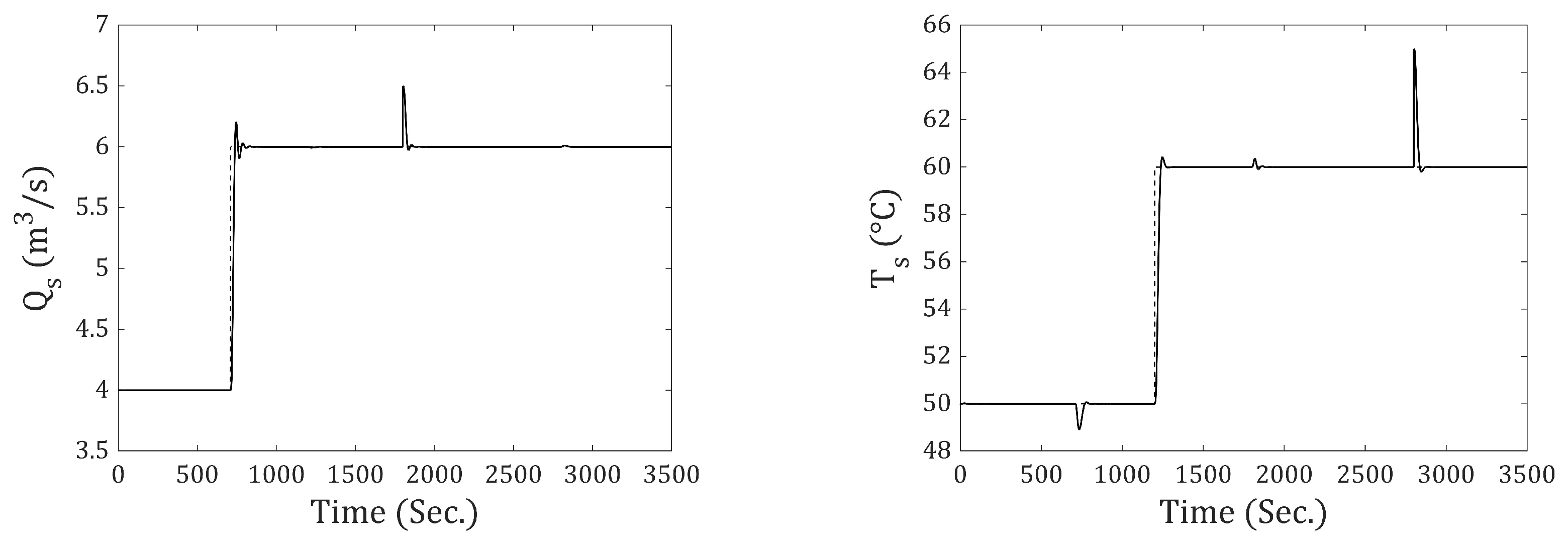
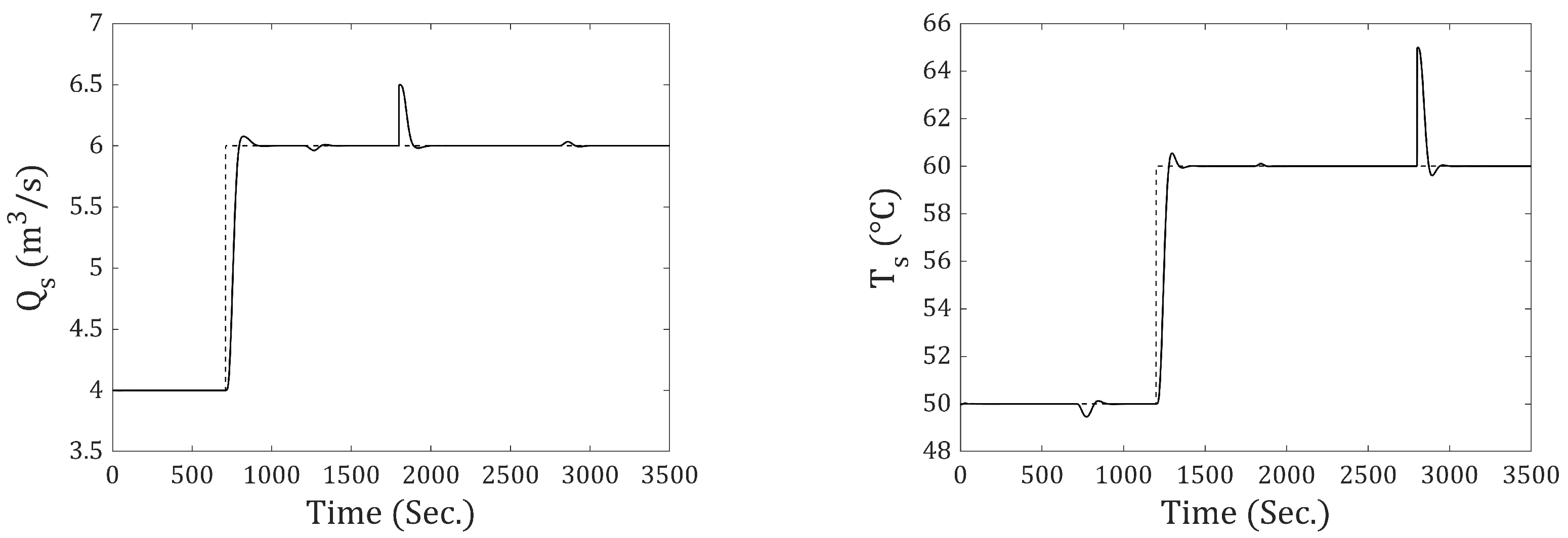
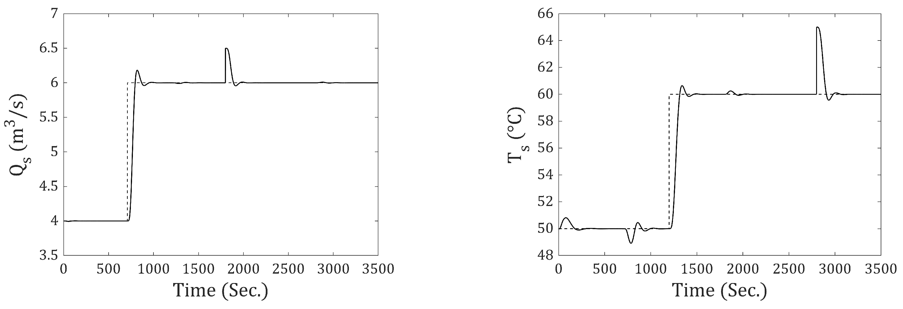
Figure 14, the responses obtained using incremental-1 through incremental-5 are shown. It is demonstrated that all of them achieve zero steady-state error in response to step-type references and disturbances (at the output). The difference among the incrementals lies in the response speed: As the incremental number increases, the response becomes slower. To better understand this behavior,
Table 5 presents the IAE and ISE values for the output flow rate and temperature for all incrementals.
11.2. Ramp-Type Reference and Output Disturbance
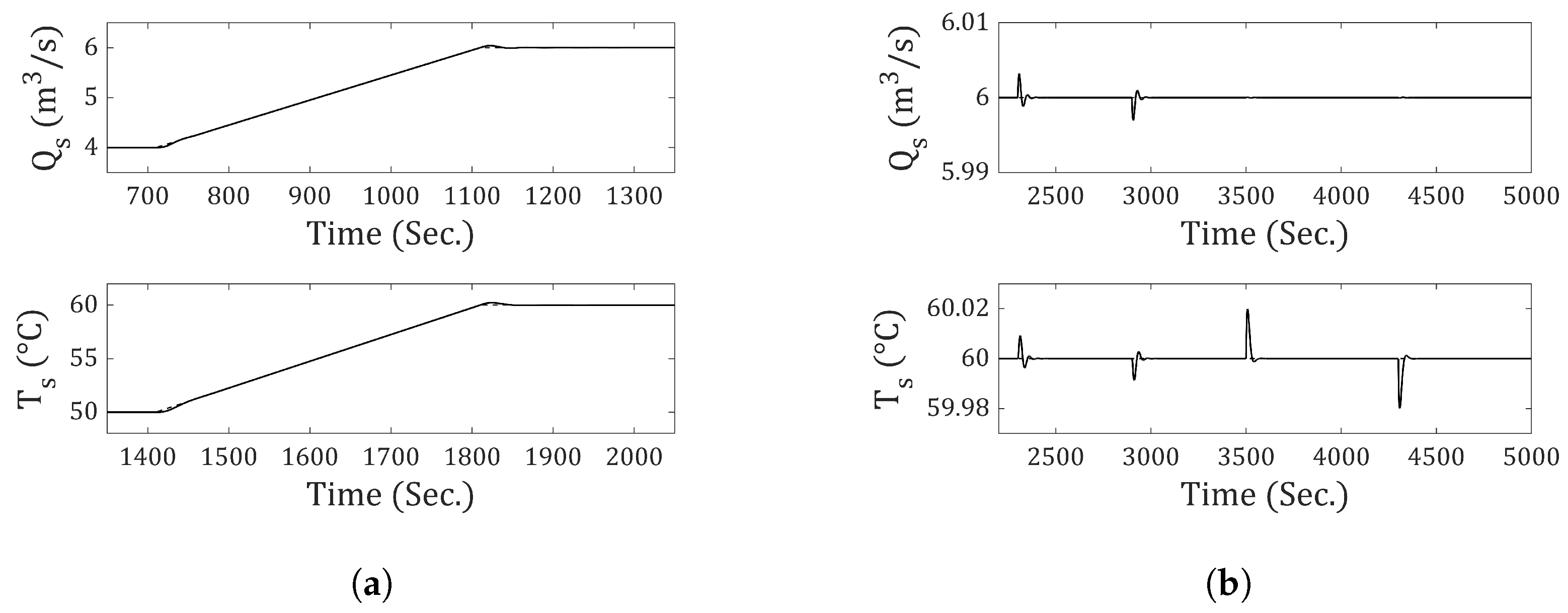
Ramp-type references and disturbances are also commonly used in the field of control, whether to smoothly start a motor or to reach a certain value in a less abrupt manner. Below are the results obtained when the system is subjected to ramp-type reference signals and output disturbances. A simulation time of 5000 s was used for all cases.
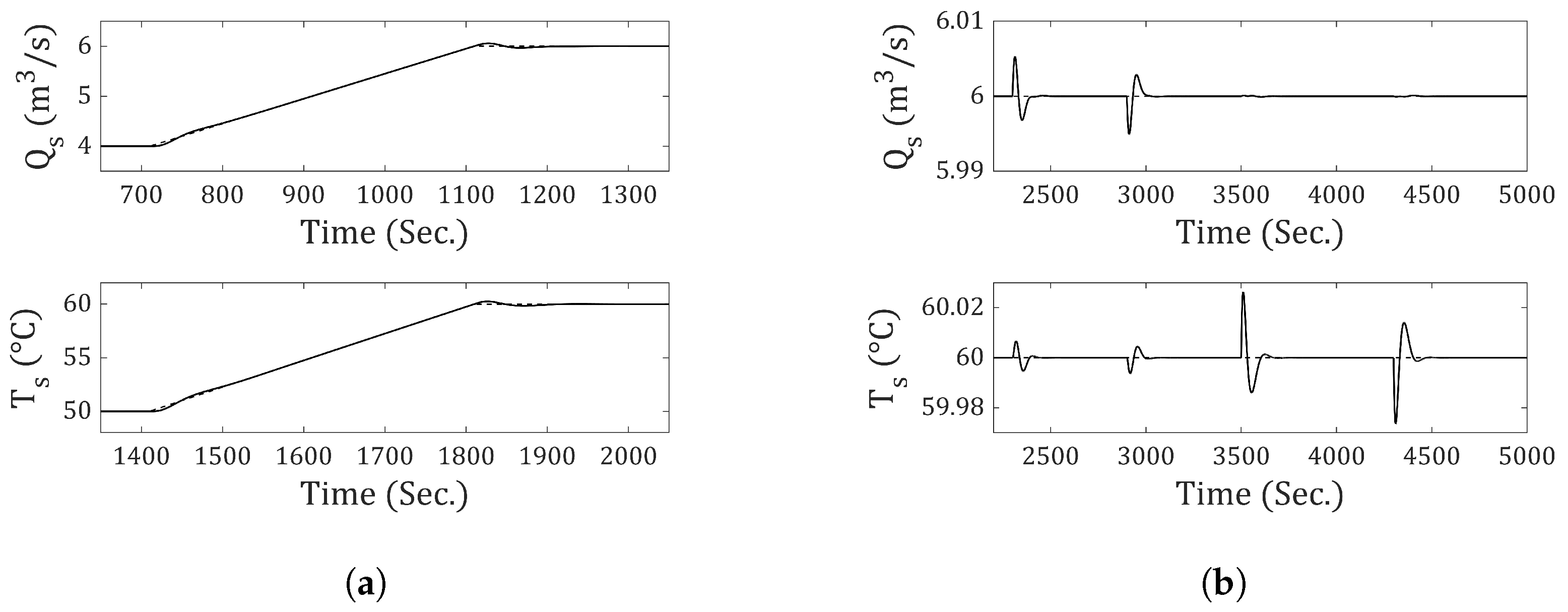
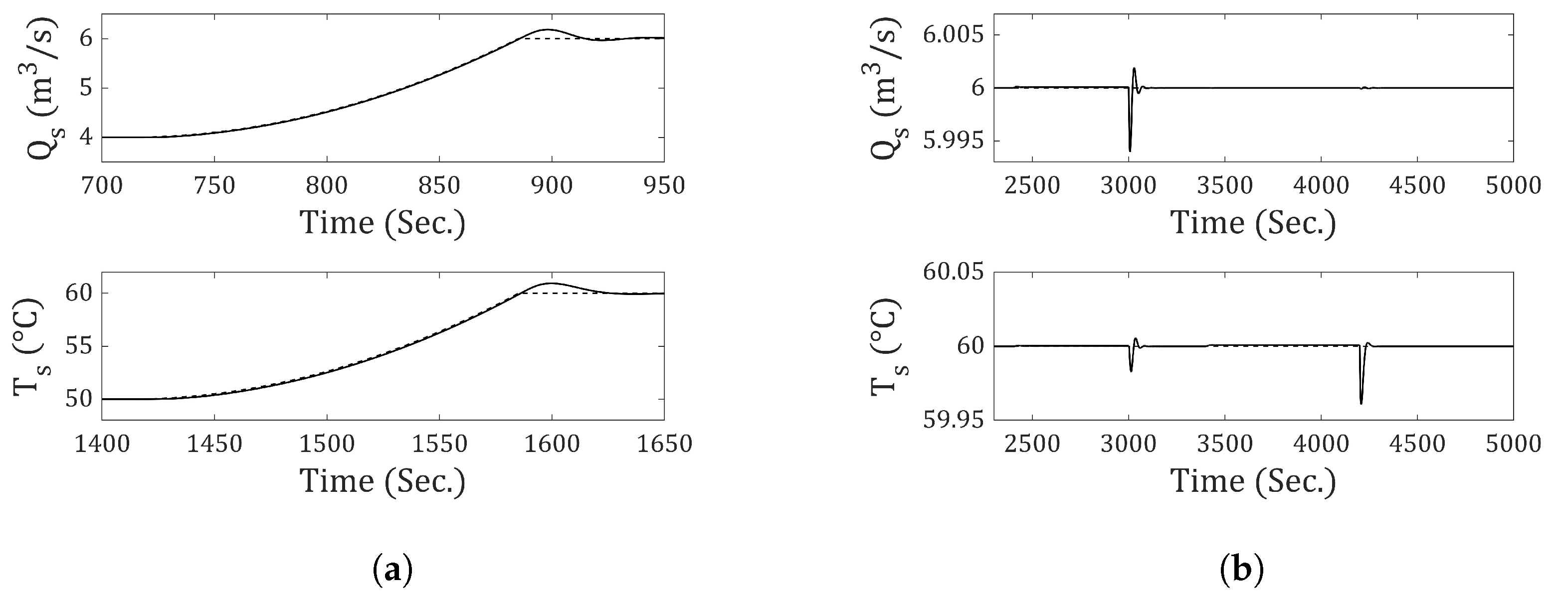
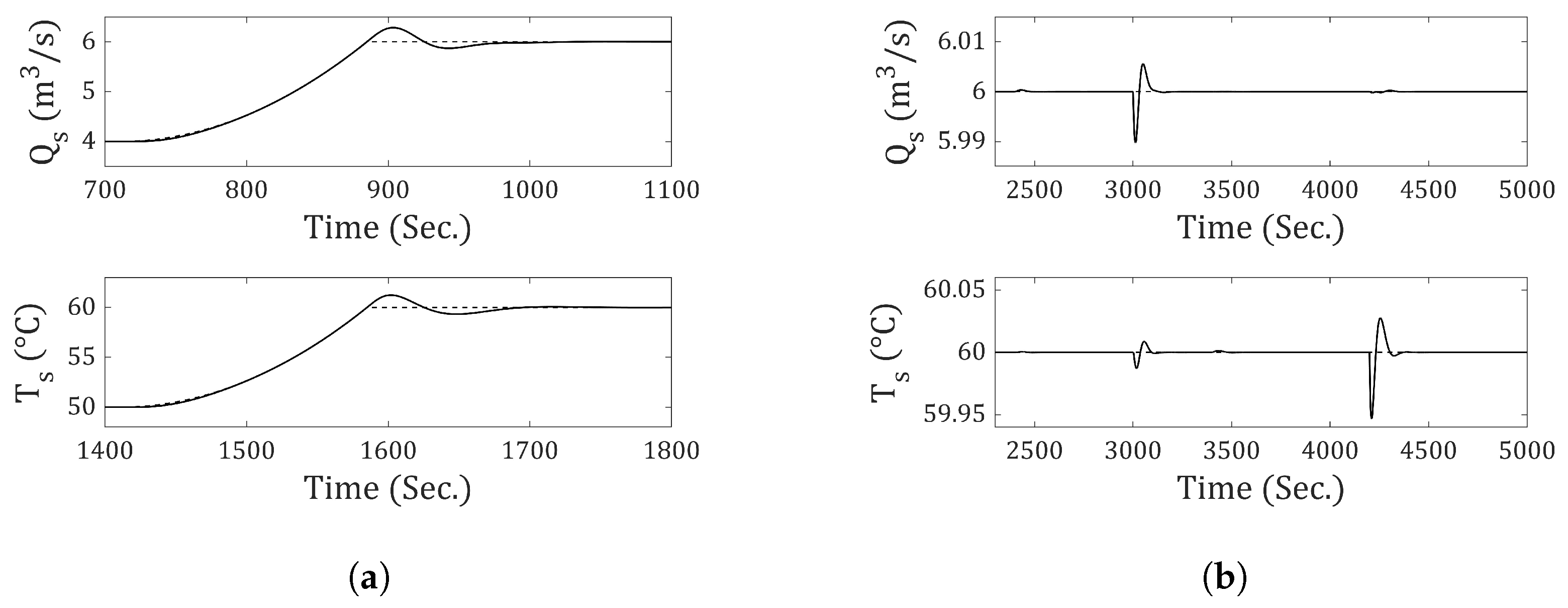
The ramp-type reference for the flow rate begins at 710 s and ends at 1110 s, with a slope of (m3/s2). For temperature, the ramp starts at 1410 s and ends at 1810 s, with a slope of (°C/s). In both cases, the final value reached is maintained until the end of the simulation.
The ramp-type disturbance for the flow rate starts at 2300 s and ends at 2900 s, with a slope of (m3/s2). For temperature, the ramp begins at 3500 s and ends at 4300 s, with a slope of (°C/s). In both cases, the final value reached is maintained until the end of the simulation.
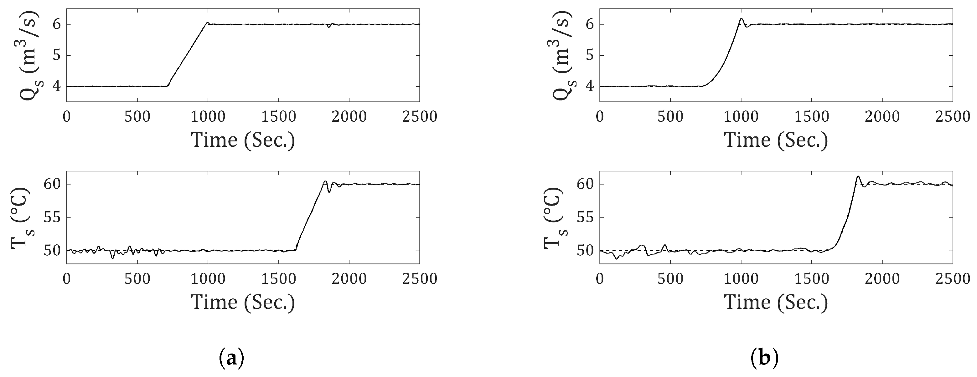
Figure 15 presents the results using incremental-1. This incremental does not achieve zero steady-state error in response to ramp-type references and output disturbances. It can be observed that the response attempts to follow the ramp but consistently exhibits an error. In contrast, when using incremental-2, zero steady-state error is achieved in response to ramp-type references and output disturbances (see
Figure 16). The same behavior is observed with incremental-3 (see
Figure 17) and beyond.
11.3. Second-Order Type Reference and Output Disturbance
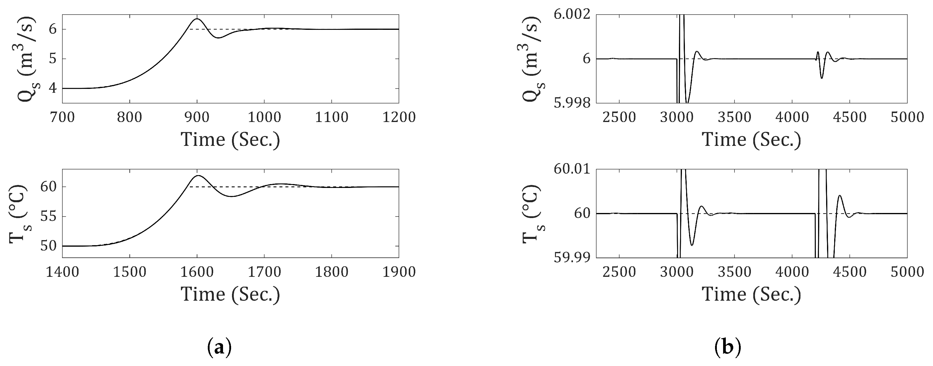
In order to verify the performance of incremental-3, the system is subjected to second-order output references and disturbances. The results are presented for a simulation that spans 5000 s.
The second-order reference for the flow rate starts at 710 s and ends at 885 s, ranging from 4 (m3⁄s) to 6 (m3
⁄s). For temperature, it ranges from 50 (°C) to 60 (°C), starting at 1410 s and ending at 1585 s. In both cases, the final value is maintained until the end of the simulation.
The second-order output disturbances for the flow rate begin at 2400 s and end at 3000 s, ranging from 0 (m3⁄s) to (m3⁄s). For temperature, the disturbance ranges from 0 (°C) to 5 (°C), starting at 3400 s and ending at 4200 s. In both cases, the final value is maintained until the end of the simulation.
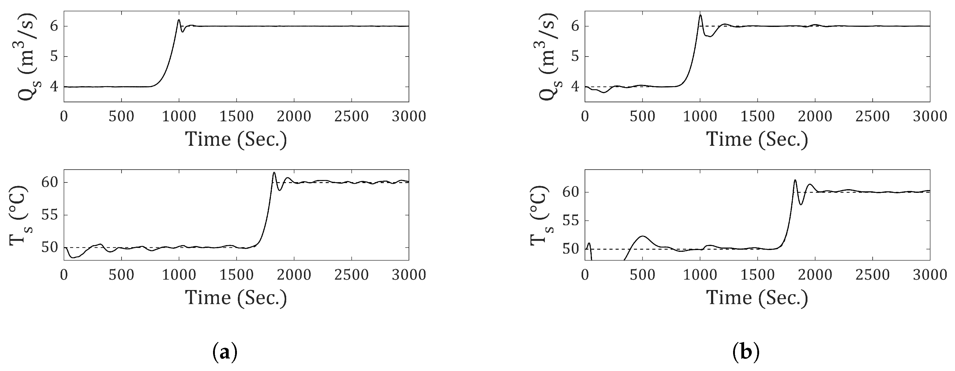
Figure 18 presents the results obtained using incremental-2. This incremental does not achieve zero steady-state error in response to second-order output references and disturbances. The response attempts to follow the parabolic input but consistently exhibits an error.
In contrast, when using incremental-3, zero steady-state error is achieved for second-order output references and disturbances (see
Figure 19). It can be observed that the response successfully follows the parabolic trajectory in both the flow rate and the output temperature.
11.4. Third-Order Type Reference and Output Disturbance
Similarly, the performance of the incremental-4 will be evaluated by subjecting the system to third-order reference inputs and output disturbances. The results are presented for a simulation time of 5000 s.
The third-order input for the flow rate starts at 710 s and ends at 885 s, increasing from 4 (m3⁄s) to 6 (m3⁄s). In the case of temperature, it rises from 50 (°C) to 60 (°C), starting at 1410 s and ending at 1585 s. In both cases, the final value reached is maintained until the end of the simulation.
The third-order output disturbances for the flow rate begin at 2400 s and end at 3000 s, ranging from 0 (m3⁄s) to (m3⁄s). For temperature, the disturbance goes from 0 (°C) to 5 (°C), starting at 3400 s and ending at 4200 s. In both cases, the final value is held constant until the simulation ends.
Figure 20 presents the results obtained using the incremental-4 approach. This incremental achieves zero steady-state error in response to third-order references and output disturbances. The system output successfully follows the reference in both flow rate and temperature.
11.5. Fourth-Order Type Reference and Output Disturbance
Finally, the performance of incremental-5 is evaluated by subjecting the system to fourth-order reference inputs and output disturbances. The simulation spans a duration of 6000 s.
The fourth-order input for the flow rate starts at 710 s and ends at 985 s, increasing from 4 (m3⁄s) to 6 (m3⁄s). In the case of temperature, it rises from 50 (°C) to 60 (°C), starting at 1610 s and ending at 1810 s. In both cases, the final value reached is maintained until the end of the simulation.
The fourth-order output disturbances for flow begin at 3000 s and end at 3600 s, ranging from 0 (m
3⁄s) to
(m
3⁄s). For temperature, the disturbance ranges from 0 (°C) to 5 (°C), starting at 4000 s and ending at 4800 s. In both cases, the final value reached is maintained until the end of the simulation.
Figure 21 presents the results obtained using incremental-5. This incremental achieves zero steady-state error in response to fourth-order output references and disturbances. The system’s response accurately follows the reference in both output flow and temperature.
11.6. Input Disturbances
Disturbances can occur not only at the output of the system but also at the input. Therefore, it is important to analyze all possible disturbances that the system may experience.
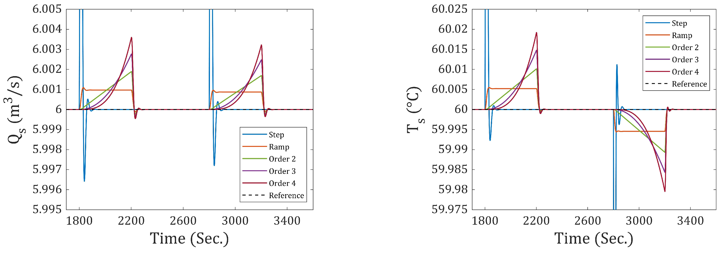
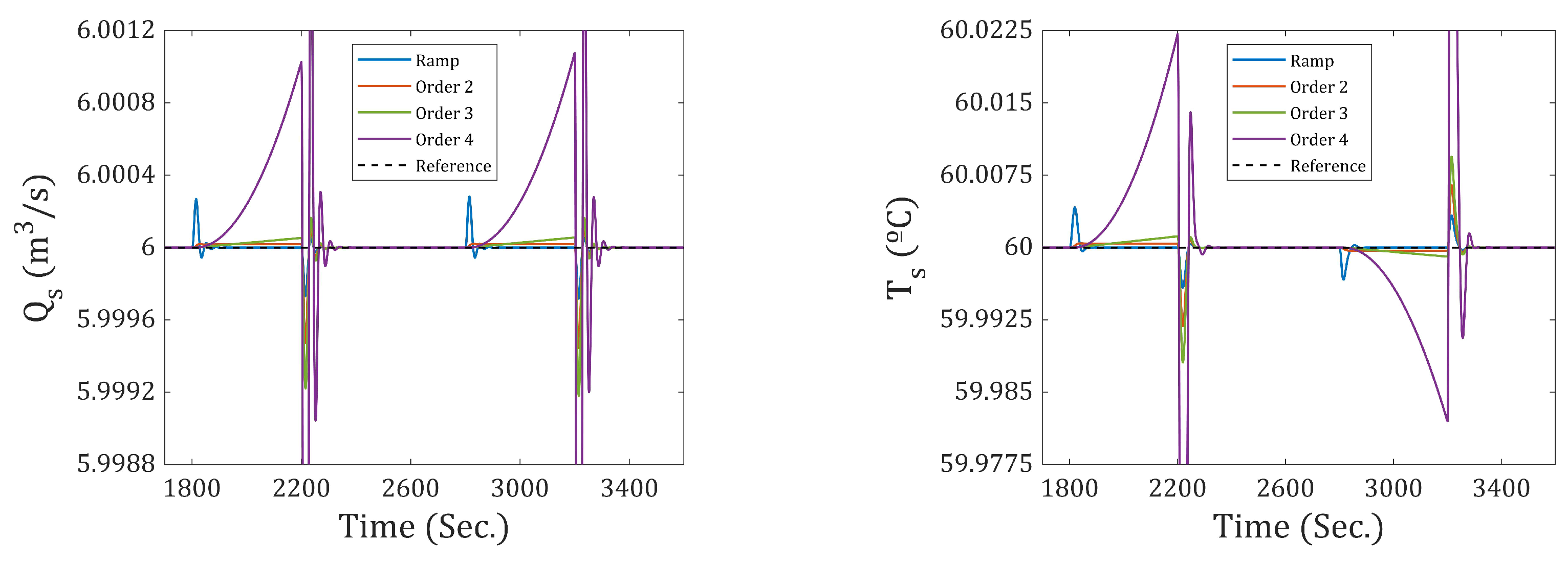
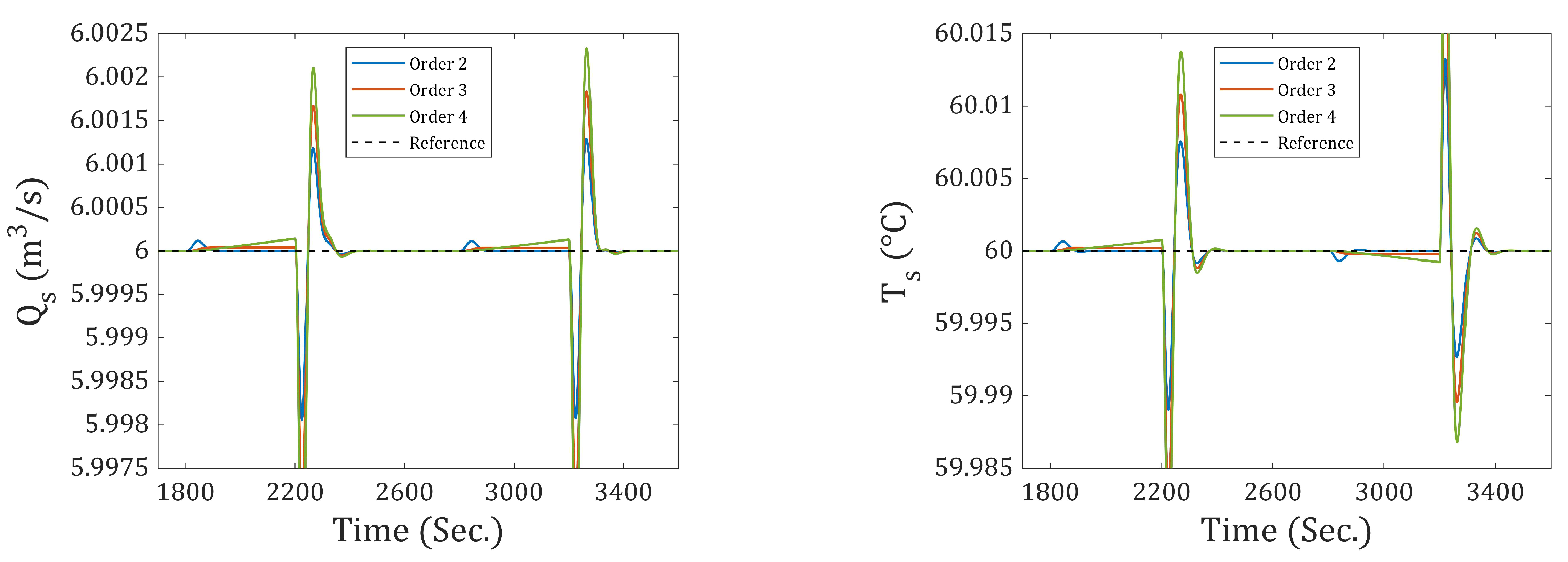
The system will be analyzed starting from the point where it reaches the state [ = 6 (m3⁄s), = 60 (°C)]. Once this state is reached, disturbances will begin to be applied to the motorized valve signals and . The step-type input disturbances for and occur at 1800 and 2800 s, respectively, each with an amplitude of . For the remaining disturbances (ramp, second-order, third-order, and fourth-order), the signal starts at 1800 s and ends at 2200 s, while starts at 2800 s and ends at 3200 s. All disturbances have an amplitude of . The simulation time for incrementals-1, 2, and 3 is 3600 s.
Figure 22 shows the responses of
and
. It can be observed that under a step-type input disturbance, the system exhibits zero steady-state error. However, as the order of the disturbance increases, the error also increases. Similarly,
Figure 23 shows the responses of incremental-2, which exhibit zero steady-state error under a ramp-type disturbance. Conversely, as with incremental-1, the error increases as the order of the disturbance increases.
Figure 24 displays the system’s response using incremental-3. In this way, zero steady-state error is achieved for disturbances of order N-1 when using incremental-N.
11.7. Load Disturbances
Load disturbances occur when changes affect the system’s behavior by modifying one of its parameters, such as the discharge coefficient of the outlet flow rate , or the temperature of one of the inlet flow rates ( or ). The following section details these possible load disturbances and shows how the system responds to them:
In this study, a value of equal to 1 was used. In this scenario, this parameter will be disturbed such that at second 200 it decreases to a value of . This simulates a step-type disturbance, which, in real terms, would represent an object obstructing the outlet duct. For this case, the incremental-1 state model will be used, and the system will start from the point [ = 6 (m3⁄s), = 60 (°C)].
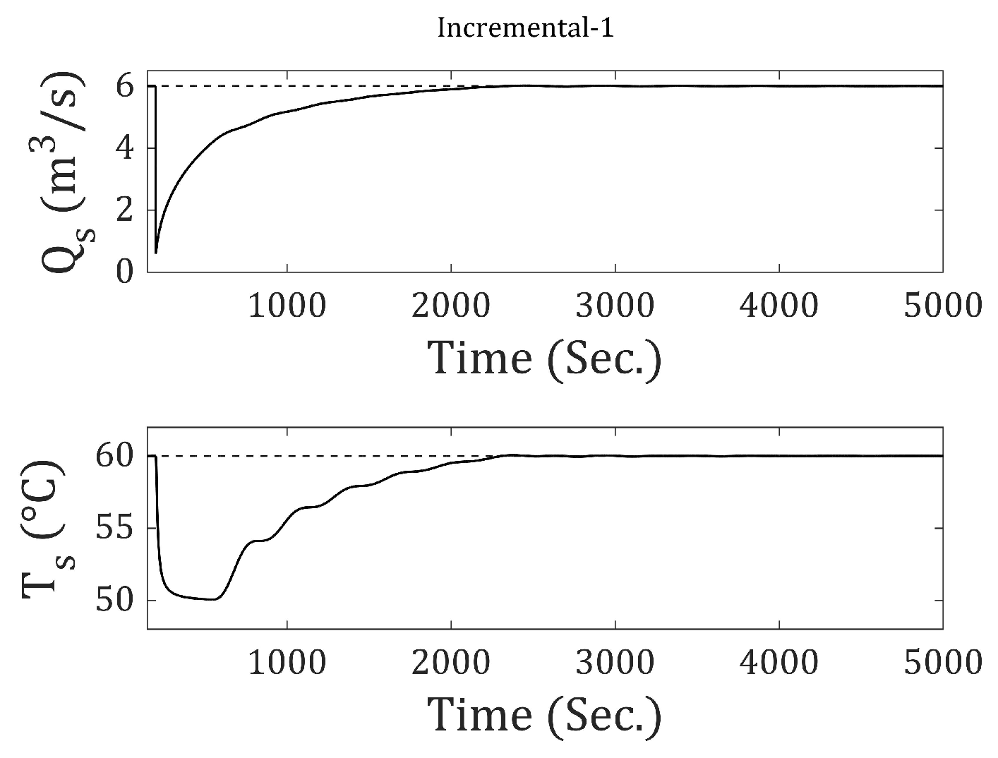
Figure 25 shows how the outlet flow rate decreases due to the obstruction, causing the system to fully open both inlet flow rates and the temperature to approach 50 (°C). As time progresses, the flow rate increases, and the temperature also rises until reaching the desired value with zero steady-state error.
Another type of load disturbance that may occur is a variation in the temperature of one of the inlet flows. For example, a malfunction in the boiler that heats the flow
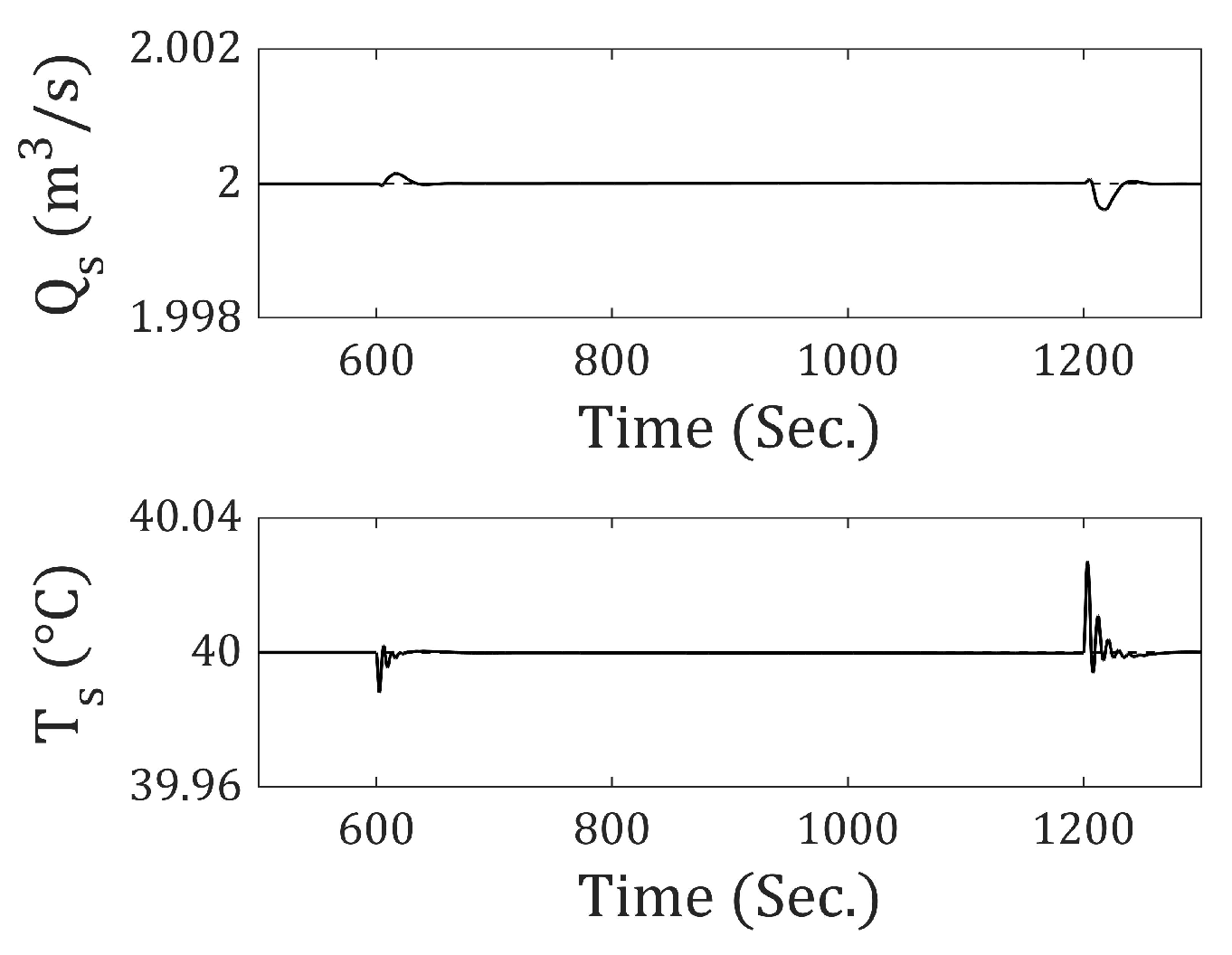
could cause its temperature to change from 90 (°C) to 60 (°C). This disturbance begins at 600 s and ends at 1200 s. It simulates a ramp-type disturbance, which, in practice, represents a gradual temperature decrease due to the failure. For this case, the incremental-2 state model will be used, starting from the point where the system reaches [
= 2 (m
3⁄s),
= 40 (°C)] (See
Figure 26).
11.8. Noise
In this section, the system will be subjected to noise in both and in order to analyze its behavior.
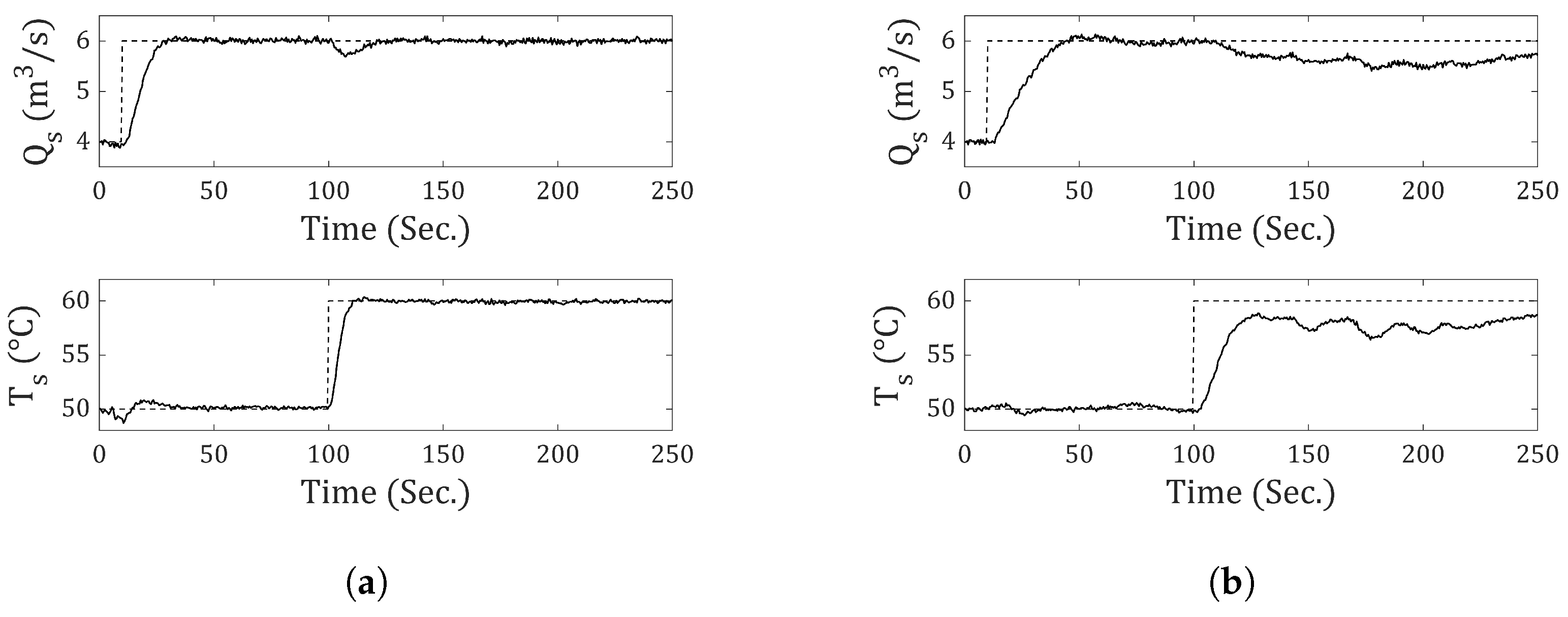
Figure 27 shows the responses of incremental-0 to step-type references for
and
, along with output noise of
N (
) and
N (
), respectively, where the first term is the mean of the distribution and the second is the variance. Also,
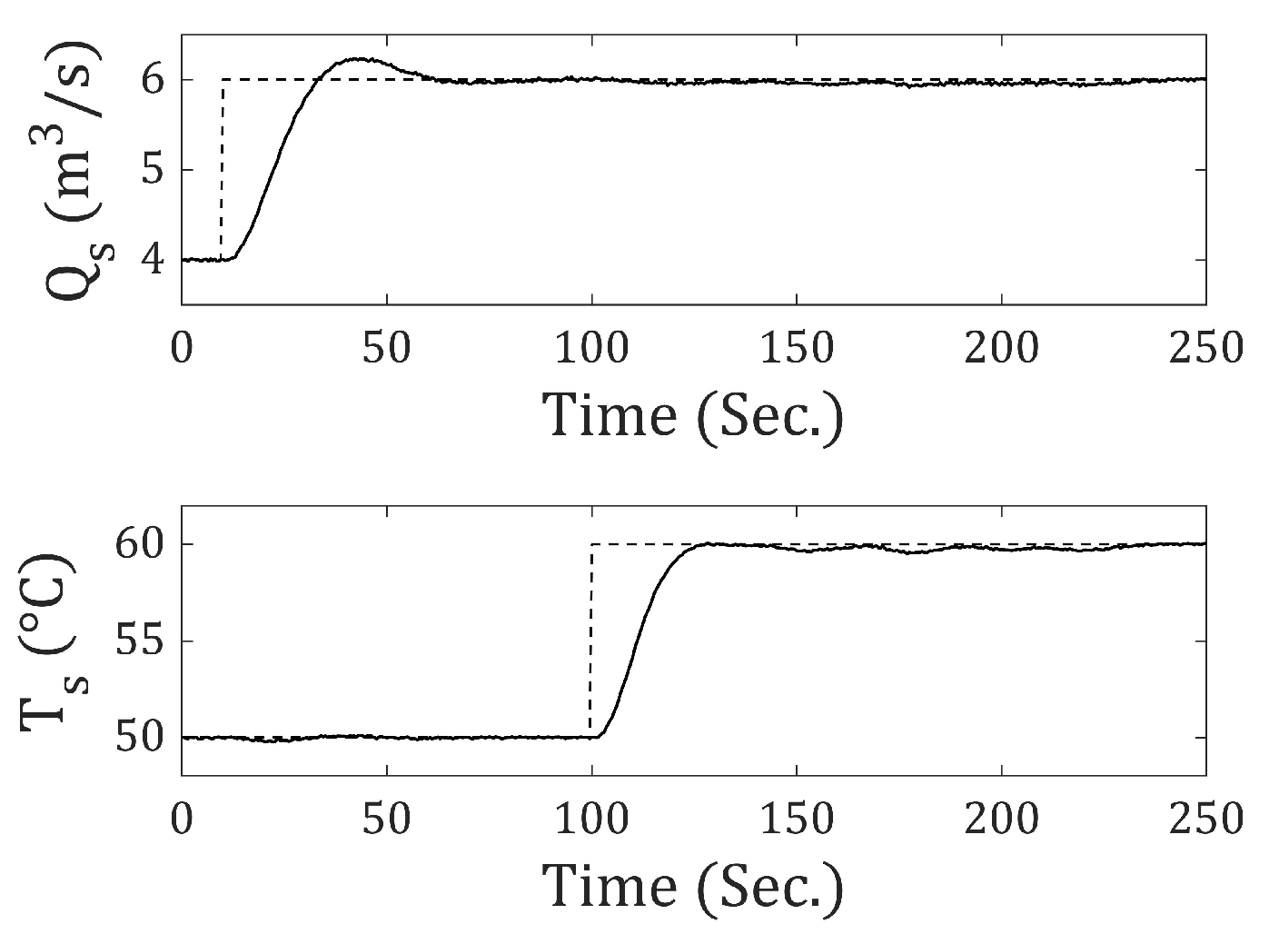
Figure 27 illustrates the system’s behavior for incremental-1 under the same inputs and noise.
It is clearly observed that Incremental-1 fails under the same noise conditions. This is because, as more incrementals are added, the noise is amplified due to the difference between the current and previous samples, which accumulates and becomes larger for the next incremental. On the other hand, if the output noise is
N (
) for
and
N (
) for
(10 times lower than in the previous case), a better response is obtained (see
Figure 28).
Figure 29 shows the response of incremental-2 to ramp-type references for
and
, as well as output noise of
N (
) and
N (
), respectively. Also,
Figure 29 shows the response of incremental-3 to second-order references for
and
, along with output noise of
N (
×
) and
N (
×
), respectively.
Meanwhile,
Figure 30 shows the response of incremental-4 to successive third-order references for
and
, along with output noise of
N (
×
) and
N (
×
), respectively. Also,
Figure 30 presents the response of incremental-5 to successive fourth-order inputs for
and
, along with output noise of
N (
×
) and
N (
×
), respectively.
It can be observed that as the number of incrementals increases, the noise variance must be reduced to prevent the system from failing drastically. Additionally, the noise has a greater effect on the output temperature.
11.9. ESC Affected by Noise
As previously shown, when noise is applied to the incremental state model, the system remains stable, although it becomes more sensitive as the number of incrementals increases. To test the ESC under more realistic conditions, it is proposed to use the ESC method with the added challenge of output noise. For the simulation, the same parameters from the ESC described in
Section 10 were used, with a simulation time of 2200 s and excessive step-type inputs. In other words, a Global ESC will be calculated while the system is affected by output noise, which follows a distribution of
N (
) for
and
N (
) for
.
Figure 31 and
Figure 32 show good system performance under noise, even when subjected to excessive step-type inputs, demonstrating a certain degree of robustness of the fuzzy LQR controller when using the incremental-1 state model.
Table 6 shows that the values of
and the RMSE of
and
are similar in both cases. Additionally, the values of the
Q matrix parameters are quite similar (see
Table 7).
11.10. Computational Burden and Real-Time Feasibility
The proposed control architecture achieves an effective compromise between control performance, adaptability, and computational feasibility by integrating incremental-N modeling, Takagi–Sugeno fuzzy systems, discrete LQR design, and Extremum Seeking Control (ESC). While PID controllers are widely adopted due to their simplicity and low computational demand, they exhibit significant limitations when applied to multivariable, nonlinear, or strongly coupled systems, such as the thermal mixing tank addressed in this study. Additionally, the tuning process for PID gains in such contexts is often heuristic and lacks robustness.
Model Predictive Control (MPC) offers a more sophisticated alternative by explicitly handling system constraints and nonlinearities through online optimization. However, this advantage comes at the cost of high computational complexity, as MPC requires solving an optimization problem at every sampling instant. Consequently, its real-time implementation becomes impractical for fast dynamic systems or platforms with limited processing capabilities.
In contrast, the methodology proposed in this work exploits the structure of the incremental-N model to manage high-order reference signals and disturbances with improved steady-state accuracy. The fuzzy state-space framework allows for an efficient representation of the system’s nonlinear dynamics, while the LQR formulation ensures stable and optimal multivariable control. Furthermore, ESC is employed exclusively as an offline optimization tool to tune the LQR weighting matrices, thereby avoiding any real-time computational overhead. Thus, the proposed approach combines the simplicity and efficiency of LQR with the adaptive tuning capabilities of ESC and the modeling flexibility of fuzzy systems, resulting in a control scheme that is both computationally efficient and well-suited for real-time applications. It offers a viable alternative to PID and MPC, particularly in scenarios where nonlinearities, multivariable interactions, and high-order dynamics must be addressed without incurring excessive computational cost.
12. Conclusions
This paper proposes the incremental-N state model for the modeling and control of nonlinear multivariable systems using Takagi–Sugeno (T–S) fuzzy models. The proposed approach ensures zero steady-state error in response to input and disturbance signals of order N-1.Furthermore, the use of the incremental-N model eliminates affine terms and addresses the challenge of computing the target state, a difficulty commonly encountered with traditional discrete-time state-space models. Moreover, the proposed approach has shown strong resilience to various adverse conditions, including disturbances at the input and load levels, as well as measurement noise. Importantly, the ESC algorithm preserves its tuning effectiveness even under noisy output conditions, highlighting the robustness and practical applicability of the overall control scheme.
A discrete Linear Quadratic Regulator (LQR) controller was designed based on the fuzzy model, requiring real-time information of the state of the system. As a result, the role of state observers is critical, since any estimation error directly impacts control performance. An optimal observer was developed to estimate the incremental-N state, given that not all states of the system are directly measurable.
The proposed control strategy was evaluated using a thermal mixing tank system as a benchmark. The simulation results confirm the achievement of zero steady-state error under reference and disturbance signals of order N-1 for incremental orders ranging from 1 to 5, while also demonstrating robust performance. However, increasing the incremental order results in slower and more oscillatory system responses, attributed to the additional integrators, which, in discrete time, correspond to poles located at in the Z-plane.
Extremum Seeking Control (ESC) was employed to optimize the Q and R weighting matrices of the discrete LQR controller. This approach significantly streamlines the tuning process, substantially reduces the design effort and computation time, and enables the identification of optimal controller parameters.
