Application of a Bi-Mamba Model for Railway Subgrade Settlement Prediction During Pipe-Jacking Tunneling

Abstract

To explore a more accurate prediction method for subgrade settlement induced by underpass construction, this study takes the existing railway project of Ningbo Yuanyi Road underpass as a case to construct a subgrade settlement prediction model based on the Mamba neural network. Using monitoring data collected using on-site automated monitoring robots as the data foundation, the prediction results of the improved transformer, long short-term memory (LSTM), time-series dense encoder (Tide), and decomposition-linear (Dlinear) neural networks are compared. The research results show that the Mean Squared Error (MSE) and Mean Absolute Error (MAE) of the proposed Bi-Mamba model are 0.279 and 0.276, respectively, demonstrating higher prediction accuracy than comparative models such as iTransformer and LSTM. Additionally, ablation experiments verify that the attention gating module in the model reduces the MSE by 9.1%, serving as a key component for improving accuracy. This study provides an advanced data-driven prediction method for subgrade settlement forecasting, offering technical references for similar engineering projects.

1. Introduction

In recent years, with the continuous improvement of the density of China’s comprehensive transportation network, the intersection nodes of highways and roads have become a key bottleneck restricting the efficiency and safety of the road network. Therefore, it is essential to transform level crossings between railways and highways into three-dimensional intersections, and rectangular top-tube tunnels under existing railways are a solution to this problem. During the construction of an underpass railway project, stress redistribution will occur in the surrounding soil, causing soil settlement and deformation, which in turn will cause deformation of the upper track and affect the safety of train operation [1,2]. Therefore, it is necessary to predict the settlement of the track and roadbed caused by the construction process and take corresponding measures to control the settlement to ensure the safety of construction and railway operation [3,4].

At present, there are two main methods used to study surface settlement in underpass projects. The first is the theoretical analysis method, which mainly includes the random medium theory [5] and analytical solution [6]. The second type is numerical analysis methods, which use finite element software to establish a simulation model to predict settlement [7]. Currently, these predictive methods and models are predominantly applied in isolation. Although each approach possesses distinct advantages and applicable scenarios, the absence of a multi-source data integration mechanism impedes the comprehensive extraction of complex correlation features embedded in field measurements, thereby limiting the improvement of the prediction accuracy.

With the continuous progress of computational technology, an increasing number of researchers are leveraging the robust nonlinear modeling capabilities of advanced algorithms, such as deep neural networks and adaptive support vector regression, to address the challenging issue of settlement prediction in railway underpass projects [8,9]. Ovídio used artificial neural networks to predict the surface settlement above the tunnel of Line 2 of the São Paulo Metro [10]. In order to determine the appropriate model for predicting the maximum surface settlement caused by shield tunneling, Chen et al. [11] compared the prediction effects of artificial neural network (ANN) and recurrent neural network (RNN). The results show that the RNN exhibits higher accuracy in modeling the spatiotemporal correlation of settlement sequences, but its inherent defect—namely, the exponential decay of gradients with increasing iteration steps (the gradient vanishing problem)—leads to a significant decrease in the learning efficiency of the model’s dynamic response to long-term construction parameters. Li Tao’s team proposed a method for predicting surface settlement during multi-stage excavation of subway tunnels based on the VMD–GRU hybrid model. This model can effectively capture the dynamic response characterized by sudden deformation fluctuations during the construction process by integrating variational mode decomposition and gated recurrent units [12]. To address the accuracy problem of settlement prediction during the operation phase of concrete face rockfill dam (CFRD), HU et al. proposed a multi-monitoring point collaborative modeling method based on optimized long short-term memory network (LSTM), which effectively integrated the spatiotemporal correlation characteristics and significantly improved the accuracy and stability of settlement prediction [13].

Traditional theoretical analysis, numerical simulation, and the above-mentioned combined neural network model have achieved certain results by predicting surface settlement data.However, these methods also have some shortcomings. For example, traditional theoretical analysis methods are usually based on idealized assumptions, and it is difficult to effectively characterize the dynamic coupling effect between complex geological structures and construction parameters [14]; although numerical simulation technology can better reflect the actual engineering, its computational efficiency is limited by the selection of refined soil constitutive models, and large-scale three-dimensional simulation faces significant computing resource consumption [15]; in the field of machine learning, the classical support vector machine algorithm is subject to the quadratic programming theoretical framework, and there is a bottleneck of a sharp increase in computational complexity when processing high-dimensional and large-sample engineering data [16]. Therefore, it is urgent to optimize and upgrade existing methods. Current research is mostly limited to the static analysis of post-construction settlement results, and fails to effectively integrate dynamic construction stage settlement data, while existing railway facilities are extremely sensitive to real-time settlement responses.By incorporating time-series settlement data within the construction period into the training set, the temporal and spatial correlation laws of soil deformation can be deeply explored, and the dynamic data characteristics can be more comprehensively extracted, which can significantly improve the prediction accuracy of the model for complex settlement processes, thereby providing a scientific basis for real-time regulation during the construction process.

By comparing and analyzing the existing neural network models in the field of sequence modeling, it is found that the Mamba model is a representative of the new state space model (SSM) [17]. With its efficient long-term dependency capture capability and linear complexity characteristics, it can effectively handle nonlinear dynamic relationships in time series and capture cross-scale data dependencies. This model has been widely used in fields such as semantic segmentation [18], image classification [19], remote sensing image prediction [20], and meteorological sequence construction [21].

Based on the above research, this paper proposes a Bi-Mamba subgrade settlement prediction model based on the Mamba model. The model first performs feature conversion on the time point of each variable. The Mamba variable correlation (VC) encoding layer then uses bidirectional Mamba to encode the correlation between variables and mine the information between global variables; then, weighted fusion is performed through the attention gate unit. Finally, the temporal dependency (TD) encoding layer containing a simple feedforward network (FFN) extracts the time-dependent features and outputs the prediction results. The Mamba model has shown great potential in the field of text and image modalities, but research in the field of subgrade settlement prediction is still blank.

This paper is based on the Bi-Mamba model and the new Ningbo Yuanyi Road underpass under the existing railway project. The real-time monitoring data during the construction period is integrated to carry out subgrade settlement modeling and prediction, and the LSTM, iTransformer, Tide, and DLinear models are used for comparative analysis to verify the reliability of the Bi-Mamba model in the settlement prediction task.

2. Monolithic Framework

Given the pronounced time-series characteristics of subgrade settlement data, this study develops a Bidirectional State Space Modeling Framework (Bi-Mamba) based on settlement monitoring data (as illustrated in Figure 1). The proposed model employs a multi-level feature extraction mechanism to accurately capture implicit temporal dependencies and dynamic evolution patterns within data sequences, enabling effective fusion of temporal features with influencing factors. Leveraging the dynamic weight allocation capability of attention-gating mechanisms, the model can precisely quantify the contribution of each influencing factor to settlement deformation while investigating the underlying causes of deformation effects. The Bi-Mamba framework demonstrates capability for advanced prediction of subgrade settlement trends during construction processes, enabling timely activation of safety warning systems. This innovation not only enhances construction efficiency and reduces project costs, but more importantly provides reliable technical support for ensuring construction quality and safeguarding the operational safety of existing railway lines.

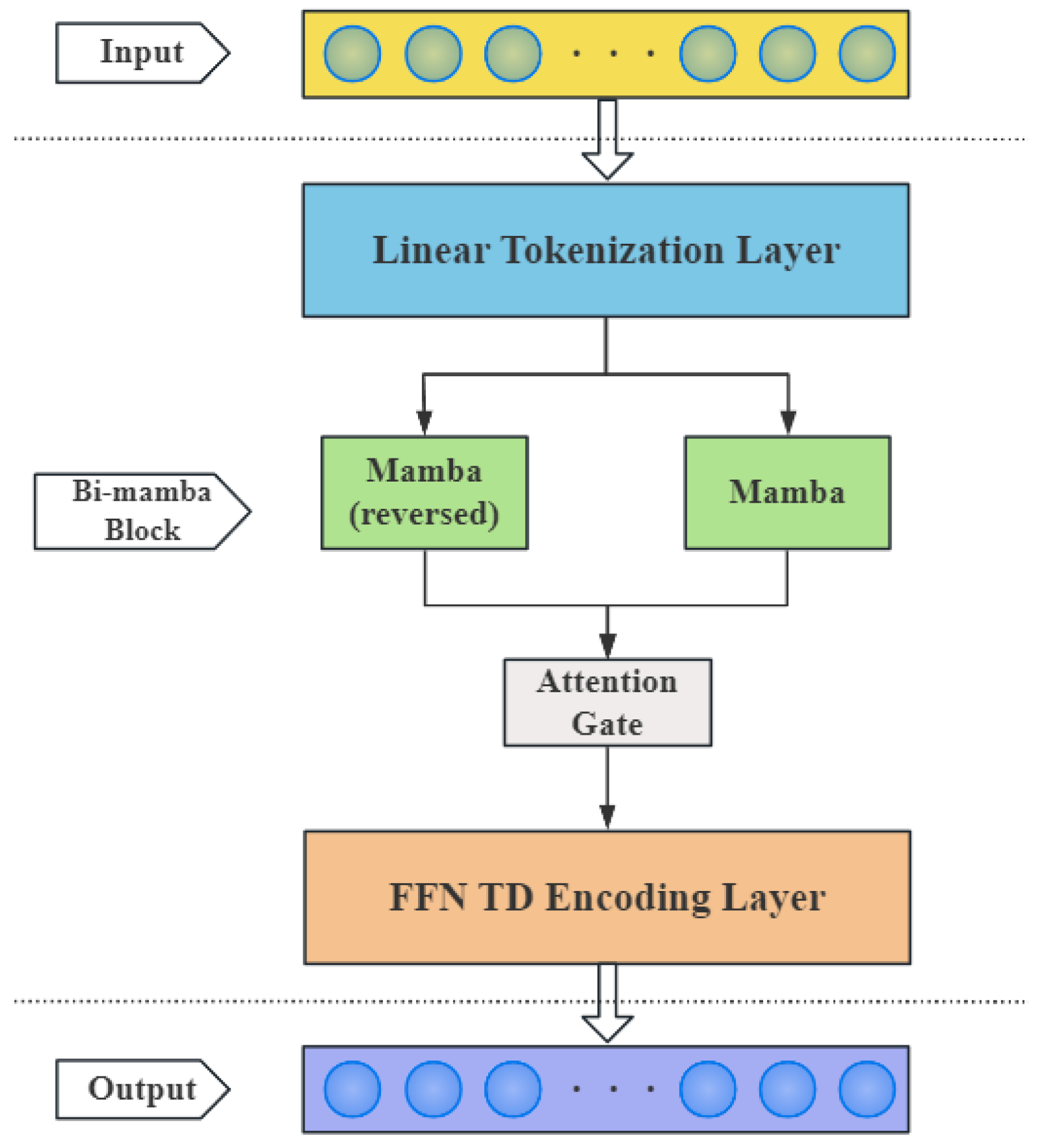
3. The Establishment of Railway Subgrade Settlement Model Based on Bi-Mamba

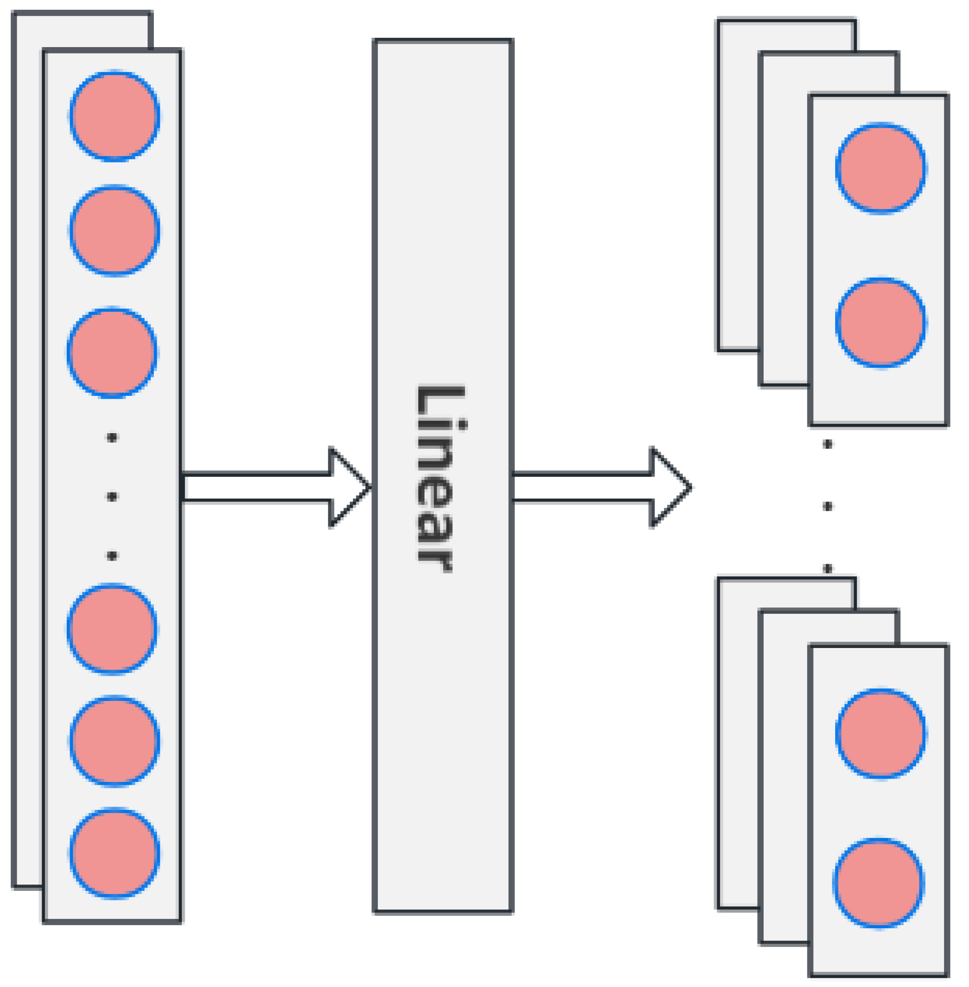
3.1. Linear Tokenization Layer

Time-series forecasting (TSF) involves using historical information to predict future states, and the input data are usually a multivariate time series. $X_{in}\in [x_1,x_2,\dots ,x_L]\in {\mathbb{R}}^{L\times N}$ [22]. After the original data are input into the Linear Tokenization Layeras illustrated in Figure 2), the input time series is first labeled and converted into a standardized feature representation suitable for deep model processing. This design is similar to the tokenization idea in natural language processing (NLP). This layer maps the multivariate observations at each time point to the latent space through linear transformation, forming a “feature label” sequence, laying the foundation for subsequent spatiotemporal feature extraction. The core operation of this layer is a single linear transformation, and its mathematical expression is:

$$X_{\mathrm{tok}}=Linear(Batch\left(X_{\mathrm{in}}\right))$$

(1)

In the equation, $X_{tok}$ is the output of the layer.

3.2. Bi-Mamba Block

Mamba is a selective state space model. As an improvement of the S4 (structured state space sequence model), it introduces a data-dependent selection mechanism and a hardware-aware parallel algorithm to efficiently capture dependencies in long sequences while maintaining near-linear computational complexity. This innovation enables Mamba to significantly outperform traditional transformer and original S4 models in sequence analysis tasks [23]. The unidirectional Mamba can only capture forward dependencies, similar to the causal structure of RNN, and cannot model backward dependencies. This makes it inadequate in scenarios that require global VC, so we design a bidirectional Mamba structure for reference here [24]. The basic structure of the Mamba layer is shown in Figure 3. After receiving the output of the previous layer, the forward Mamba block processes the sequence in the original order and transforms the output through the following formula; it then models the sequence dependency through a dynamically parameterized state space model and multiplies the output of the selective SSM by the gating signal of the branch element by element.

$$X^{\prime }=\sigma (Conv(Linear\left(X_{\mathrm{tok}}\right)))$$

(2)

$$X^{″}=\sigma (Linear\left(X_{\mathrm{tok}}\right))$$

(3)

$$\sigma \left(\mathrm{x}\right)=\mathrm{x}·sigmoid\left(\mathrm{x}\right)$$

(4)

$$h_t={\overline{A}}_t{h}_{t-1}+{\overline{B}}_t{x}_t$$

(5)

$$y_t=C_t{h}_t$$

(6)

In the equation, $X^{\prime }$ represents the value of the input SSM after branch 1 processing. Each channel is convolved independently to capture local spatial features, and then activated by the SiLU function to introduce smooth nonlinearity and enhance feature expression capabilities. $X^{″}$ indicates that branch 2 is directly activated by linear transformation and SiLU function to generate gating signal, which is directly used for the output of SSM. The backward Mamba block reverses the input sequence and inputs it to another Mamba block.

$$Y\_forward= Mamba\_forward\left(X\right)$$

(7)

$$Y\_backward= Mamba\_forward\left(X\right)$$

(8)

Bidirectional Mamba encoding finally generates $Y\_forward$ and $Y\_backward$.

3.3. Attention Gate

In the previous layer, we use a bidirectional Mamba layer to process the correlation (VC) between variables. If it is simply added after processing, it will lack the ability to distinguish the dynamic importance of the variables, so we add an attention gating unit after the Bidirectional Mamba output [25]. We adjust the fusion ratio of the forward and reverse Mamba outputs by calculating dynamic weights, concatenating the features of the two Mamba outputs, calculating the weights through the attention gating network, and finally performing weighted fusion of the two outputs based on the weights. The calculation formula is as follows:

$$Z=Concat(Y\_forward,Y\_backward)$$

(9)

$$A=W\_2·\sigma (W\_1·Z+b\_1)+b\_2$$

(10)

$$\alpha =Sigmoid\left(A\right)$$

(11)

$$Y\_gated=\alpha \otimes Y\_forward+(1-\alpha )\otimes Y\_backward$$

(12)

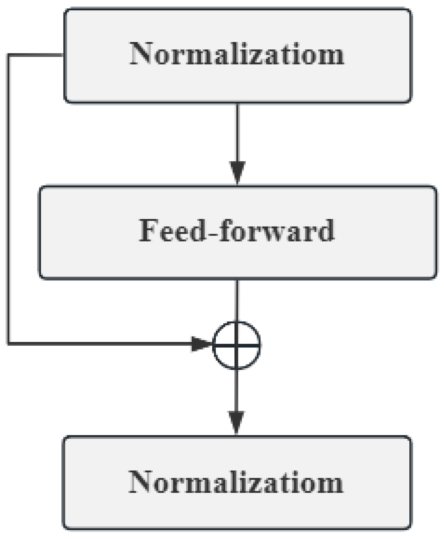
3.4. FFN TD Encoding Layer

The FFN TD encoding layer (feedforward network time dependency encoding layer) is the core module in the model responsible for extracting time-series temporal dependencies (TD). After capturing the correlation (VC) between variables, it can further model the time-series characteristics of each variable to generate accurate prediction results [26]. The FFN TD encoding layer mainly consists of two normalization layers and a feedforward network layer. The FFN TD encoding layer is shown in Figure 4.

4. Project Examples

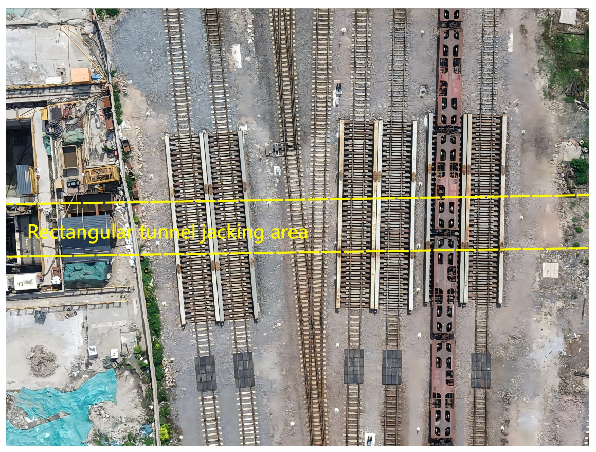
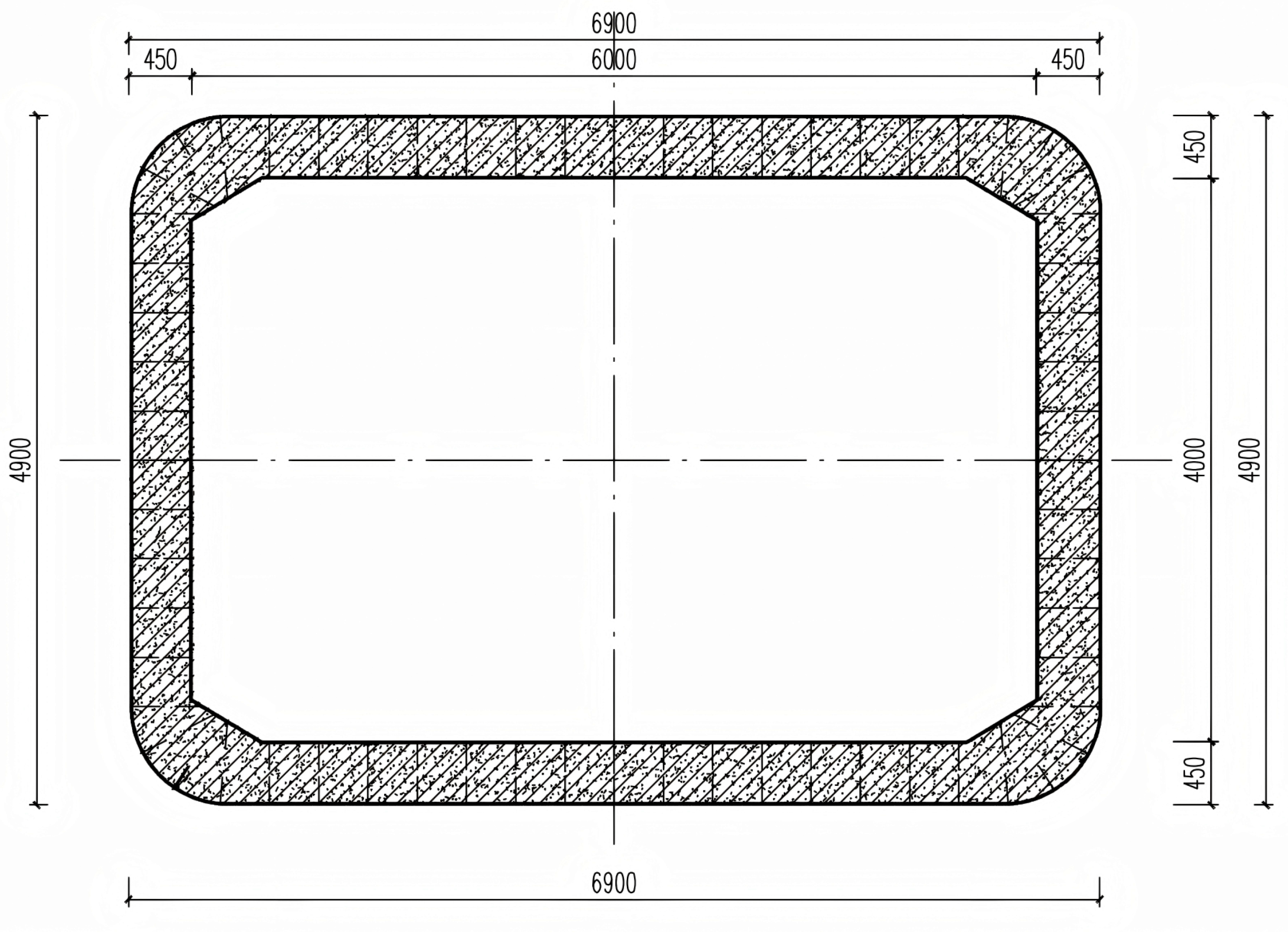
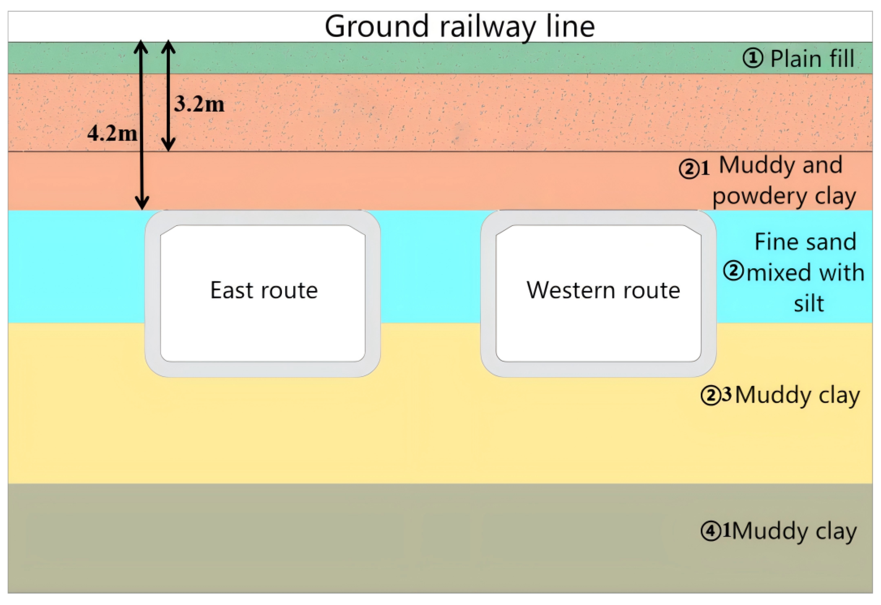
4.1. Project Overview

This study is based on the Ningbo Yuanyi Road underpass project that crosses existing railway lines. The underpass section employs a rectangular pipe-jacking method, with the tunnel crossing located at meleage K20 + 461. The rectangular jacking structure comprises dual cavities orthogonal to the railway alignment. The railway tracks (numbered 1 to 7) are traversed in the jacking direction from Track 7 to Track 1, with Figure 5 showing the construction layout plan. Prior to underpass construction, the existing railway subgrade was reinforced using MJS (Metro Jet System) grouting. During the underpass operation, D-type temporary beams were installed for pre-reinforcement of the active railway lines. The rectangular tunnel has a clear span of 6.0 m and a clear height of 4.0 m, with uniform thicknesses of 0.45 m for the top slab, bottom slab, and sidewalls. Detailed dimensions of the jacking tunnel are provided in Figure 6 (all values are presented in millimeters).

The geological parameters of the jacking soil layer mainly include the physical and mechanical parameters of the top and bottom strata of the tunnel, such as the characteristic value of the bearing capacity of the foundation soil, compression modulus, cohesion, friction angle, and porosity ratio; the soil layer is divided into five layers from the bottom. The soil layers from top to bottom are plain fill, muddy and powdery clay, fine sand mixed with silt, muddy clay, and muddy clay.

Table 1. Soil parameters table.

Name of Soil Layer	Characteristic Value of Bear Capacity/kpa	Compression Modulus/Mpa	Cohesion/kpa	Friction Angle/°	Void Ratio
Plain fill	/	/	/	/	/
Muddy and powdery clay	60	4.5	12.2	10.5	1.028
Fine sand mixed with silt	110	6.6	12.2	19.5	0.648
Muddy clay	60	2.8	10.9	8.6	1.217
Muddy clay	65	2.7	15.9	9.8	1.330

lists the soil layer parameters. Figure 7 is a schematic diagram of the cross-section of the pipe-jacking tunnel and the existing railway line.

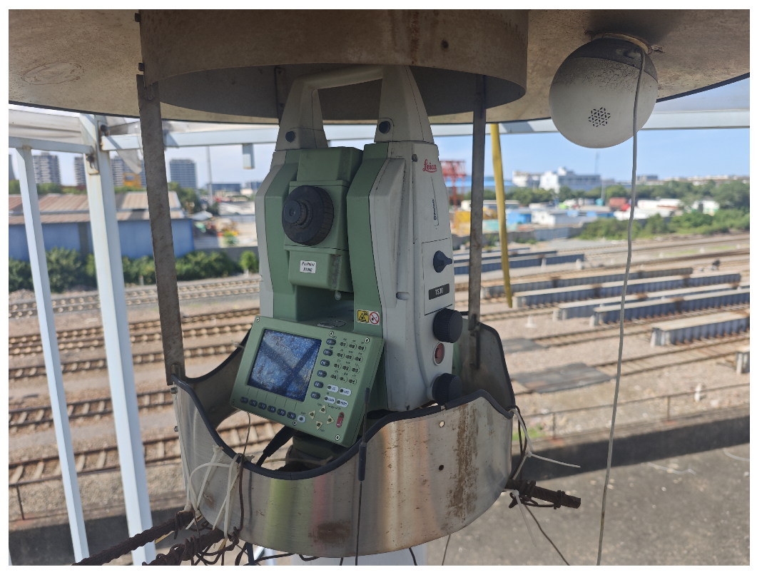
4.2. Data Acquisition

To effectively predict and analyze track and subgrade settlement deformation during construction, ensuring the safe and smooth implementation of the rectangular pipe-jacking operation, on-site monitoring has become an indispensable component of this project. Based on field conditions, the monitoring points are arranged as follows: a pier monitoring point is arranged at each end of the D24 type temporary beam, six monitoring points are arranged at equal intervals on the temporary beam, one group of monitoring points is arranged at an interval of 10 m for each track of the railway line, and five groups of roadbed monitoring points are arranged on the roadbed between the tracks. The schematic layout of monitoring points is shown in Figure 8.

Field monitoring was conducted using an intelligent automatic monitoring method, with a fully automated measuring robot as the core data acquisition device. Figure 9 shows the on-site observation device diagram. The measuring robot employed a Leica TS30 Ultra-High Precision Total Station, featuring an angular measurement accuracy of 0.5 s and a distance measurement accuracy of 0.6 mm + 1 ppm. Data are automatically collected every hour. Due to the influence of weather and train obstruction during data collection, the data may be missing or abnormal. We use linear interpolation to fill these missing values. The data collected was then organized into a dataset for this study, resulting in a monitoring dataset consisting of 3212 samples. Each sample comprised 82 input parameters and one output parameter, both of which represented the displacement of the sample point in the direction perpendicular to the ground. The dataset follows the principle of using 70% of the data as the training set and 30% as the validation set.

4.3. Experimental Analysis

4.3.1. Model Evaluation Metrics

The core process of model prediction is to fit the data to build a model, and then predict subsequent data points based on the established model. Fitting is the key link in modeling, and prediction is the final output of this process. This article uses mean squared error (MSE) and mean absolute error (MAE) as evaluation indicators. The calculation formula is as follows:

$$\mathrm{MSE}={\displaystyle \frac{1}{n}}\sum _{i=1}^n{(y_i-{\widehat{y}}_i)}^2$$

(13)

$$\mathrm{MAE}={\displaystyle \frac{1}{n}}\sum _{i=1}^n\left|y_i-{\widehat{y}}_i\right|$$

(14)

where $y_i$ is the true value, ${\widehat{y}}_i$ is the predicted value, and n is the number of samples. The smaller the MSE and MAE, the closer the model’s predicted value is to the true value.

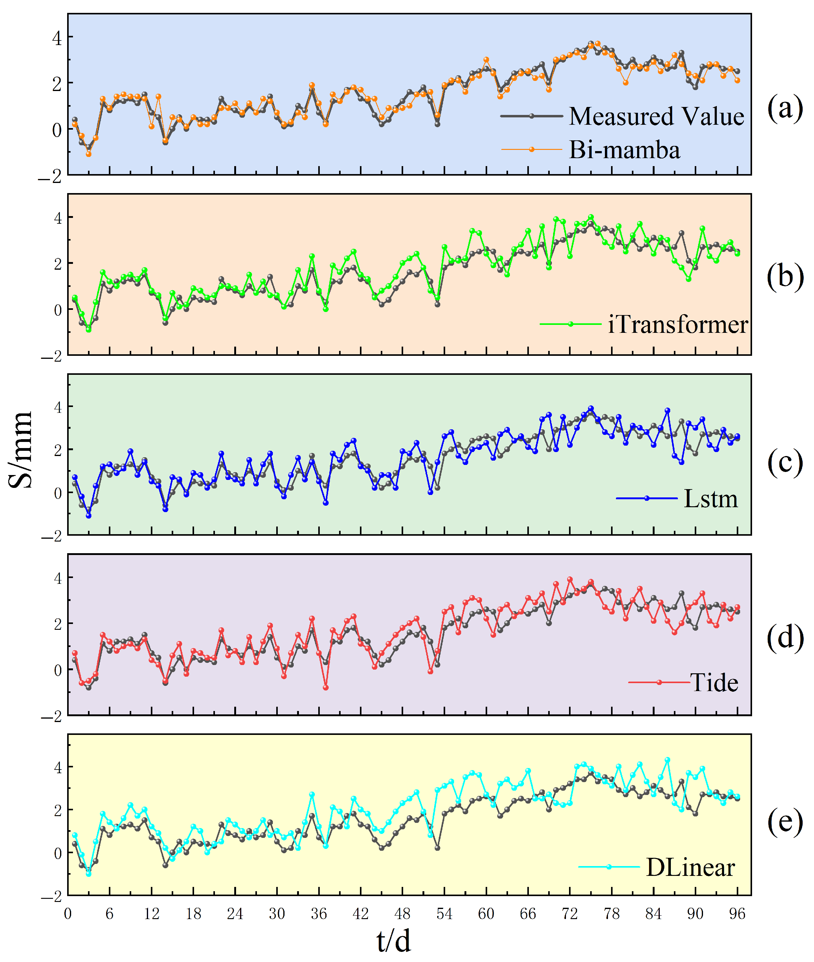
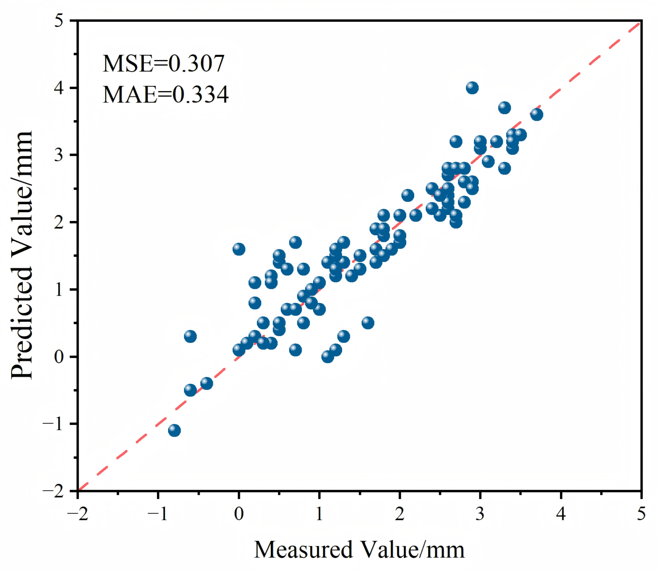
4.3.2. Prediction Results

This experiment uses the PyTorch1.4 deep learning framework to build the Bi-Mamba model and obtain relevant results. The specific implementation is based on the Python3.6 programming language and is completed through the VSCode development platform in the Ubuntu 22.04 operating system environment. The experimental hardware configuration is a NVIDIA RTX 4090 graphics card, Intel (R) i7-13700k processor, and 60 GB memory. The network training uses the Adam optimizer, with mean square error loss (MSELoss) as the loss function, and the learning rate is set to 0.001. This paper uses the Bi-Mamba model to predict and analyze the monitoring point: L1-1. The prediction results are shown in Figure 10.

4.3.3. Model Comparison Experiment

In order to verify the effectiveness of the method proposed in this paper for predicting settlement caused by underpass construction, four networks, iTransformer [22], LSTM [27], Tide [28], and DLinear [29], were selected to compare the performance of the proposed Bi-Mamba model. The input parameters and training times of iTransformer, LSTM, Tide, and DLinear are consistent with those of Bi-Mamba. The performance of the models was tested using the same test set. The comparison between the model prediction results and the actual measurement results is shown in Figure 11 and Figure 12. The MAE and MSE comparison of each model is shown in

Table 2. Model performance comparison for different forecast lengths.

	Model	Bi-Mamba		iTransformer		LSTM		Tide		DLinear
	Metric	MSE	MAE	MSE	MAE	MSE	MAE	MSE	MAE	MSE	MAE
The Forecast Length	16	0.173	0.213	0.325	0.373	0.272	0.175	0.573	0.318	0.294	0.259
	32	0.203	0.234	0.398	0.428	0.432	0.258	0.624	0.339	0.452	0.264
	64	0.255	0.273	0.435	0.455	0.681	0.382	0.641	0.341	0.723	0.402
	96	0.279	0.276	0.606	0.498	0.753	0.525	0.675	0.394	1.030	0.560

.

As shown in Table 2, the MSE and MAE values of Bi-Mamba at different prediction lengths are lower than those of other models. In particular, for high-precision long sequence prediction (such as 96 steps), the MSE value of Bi-Mamba is 0.279, which is 0.474, 0.327, 0.396, and 0.751 lower than LSTM, iTransformer, Tide, and DLinear, respectively; the MAE of Bi-Mamba is 0.276, which is 0.249, 0.222, 0.118, and 0.284 lower than LSTM, iTransformer, Tide, and DLinear, respectively. It can be seen that the accuracy of Bi-Mamba is significantly better than that of other models, indicating that the Mamba model can more accurately mine the laws of mutual influence of time-series data during the construction process in long time-series prediction, indicating that the model proposed in this paper has better fitting accuracy and prediction performance, and can more accurately predict the subgrade settlement caused by the construction of the underpass.

4.3.4. Ablation Experiment

In order to explore the effectiveness of the Attention Gate module used in this paper, an ablation experiment was conducted on a dataset of railway subsidence caused by tunnel construction. In order to verify the effectiveness of the Attention Gate, a Bi-Mamba prediction model without the Attention Gate module was constructed and tested using the dataset constructed in this paper. The test results are shown in Figure 13.

The MSE and MAE of the Bi-Mamba model without the Attention Gate module are 0.307 and 0.334, respectively, which are 0.028 and 0.058 higher, respectively, than those of the complete Bi-Mamba model. The above results show that after the introduction of the Attention Gate module, the comprehensive prediction performance of the model is significantly improved, indicating that the Attention Gate module can effectively improve the model’s ability to capture key information and dynamic relationships, and reduce the impact of redundant information on the prediction results.

5. Conclusions

This study innovatively proposes a subgrade settlement time-series prediction model based on the Bidirectional Mamba (Bi-Mamba) architecture, validated using automated monitoring data from the Ningbo Yuanyi Road underpass project that crosses existing railways, leading to the follwing conclusions:

(1)

The Bi-Mamba model demonstrates excellent alignment between predicted and actual settlement values, effectively capturing the relationship between pipe jacking progress and surface subsidence. For long-sequence predictions, the model achieves MSE and MAE of 0.279 and 0.27,6 respectively, outperforming iTransformer, LSTM, Tide, and DLinear models in predictive accuracy. These results establish Bi-Mamba as a novel methodological approach for subgrade settlement prediction.

(2)

The Attention Gate mechanism significantly enhances model performance by dynamically adjusting feature fusion weights through computed attention coefficients.

(3)

The study could further incorporate soil information; for example, the cohesion of soil layers can be incorporated as input variables into the model, to predict foundation settlement under different geological conditions.

References

1. Chen, R.; Wang, Z.; Wu, H. Risk assessment for shield tunneling beneath buildings based on interval improved TOPSIS method and FAHP method. J. Shanghai Jiao Tong Univ. 2022, 56, 1710–1719. [Google Scholar]
2. Jin, D.; Yuan, D.; Li, X.; Zheng, H. Analysis of the settlement of an existing tunnel induced by shield tunneling underneath. Tunn. Undergr. Space Technol. 2018, 81, 209–220. [Google Scholar] [CrossRef]
3. Hao, Z.; Zhang, H.; Zhang, G.; Xiong, W.; Wang, L. The Prediction of Ground Settlement of a Box Culvert Jacked Under the Action of an Ultra-Shallow Buried Pipe Curtain. Arab. J. Sci. Eng. 2022, 47, 12423–12438. [Google Scholar] [CrossRef]
4. Li, J.; Yan, B.; Shi, Y. The monitoring and analysis of surface subsidence of Soft soil rock large section of subway tunnel shield construction. In Proceedings of the 2nd International Conference on Energy Materials and Material Application, Changsha, China, 5–7 December 2013; pp. 78–82. [Google Scholar]
5. Hamza, M.; Ata, A.; Roussin, A. Ground movements due to the construction of cut-and-cover structures and slurry shield tunnel of the Cairo Metro. Tunn. Undergr. Space Technol. 1999, 14, 281–289. [Google Scholar] [CrossRef]
6. Li, T.Z.; Yang, X.L. Stability of plane strain tunnel headings in soils with tensile strength cut-off. Tunn. Undergr. Space Technol. 2020, 95, 103138. [Google Scholar] [CrossRef]
7. Ding, D.; Yang, X.; Lu, W.; Liu, W.; Yan, M. Numerical Analysis on Deformation of Adjacent Structures due to Metro Station Construction by Enlarging Large-diameter Shield Tunnel. In Proceedings of the International Conference on Civil Engineering and Building Materials, Kunming, China, 31 October–3 November 2011; pp. 1196–1200. [Google Scholar]
8. Huang, Y.; Zhang, T.; Yu, T.; Wu, X. Support vector machine model of settlement prediction of road soft foundation. Rock Soil Mech. 2005, 26, 1987–1990. [Google Scholar]
9. Kirts, S.; Nam, B.H.; Panagopoulos, O.P.; Xanthopoulos, P. Settlement prediction using support vector machine (SVM)-based compressibility models: A case study. Int. J. Civ. Eng. 2019, 17, 1547–1557. [Google Scholar] [CrossRef]
10. Santos, O.J.; Celestino, T.B. Artificial neural networks analysis of São Paulo subway tunnel settlement data. Tunn. Undergr. Space Technol. 2008, 23, 481–491. [Google Scholar] [CrossRef]
11. Chen, R.; Zhang, P.; Wu, H.; Wang, Z.; Zhong, Z. Prediction of shield tunneling-induced ground settlement using machine learning techniques. Front. Struct. Civ. Eng. 2019, 13, 1363–1378. [Google Scholar] [CrossRef]
12. Li, T.; Tang, T.; Liu, B.; Chen, Q. Surface settlement prediction of subway tunnels constructed by step method based on VMD-GRU. J. Huazhong Univ. Sci. Technol. 2023, 51, 48–54+62. [Google Scholar]
13. Hu, Y.; Gu, C.; Meng, Z.; Shao, C.; Min, Z. Prediction for the Settlement of Concrete Face Rockfill Dams Using Optimized LSTM Model via Correlated Monitoring Data. Water 2022, 14, 2157. [Google Scholar] [CrossRef]
14. Su, J.; Wang, Y.; Niu, X.; Sha, S.; Yu, J. Prediction of ground surface settlement by shield tunneling using XGBoost and Bayesian Optimization. Eng. Appl. Artif. Intell. 2022, 114, 105020. [Google Scholar] [CrossRef]
15. Chen, R.P.; Zhang, P.; Kang, X.; Zhong, Z.Q.; Liu, Y.; Wu, H.N. Prediction of maximum surface settlement caused by earth pressure balance (EPB) shield tunneling with ANN methods. Soils Found. 2019, 59, 284–295. [Google Scholar] [CrossRef]
16. Goh, A.T.C.; Zhang, W.; Zhang, Y.; Xiao, Y.; Xiang, Y. Determination of earth pressure balance tunnel-related maximum surface settlement: A multivariate adaptive regression splines approach. Bull. Eng. Geol. Environ. 2018, 77, 489–500. [Google Scholar] [CrossRef]
17. Wang, C.; Tsepa, O.; Ma, J.; Wang, B. Graph-mamba: Towards long-range graph sequence modeling with selective state spaces. arXiv 2024, arXiv:2402.00789. [Google Scholar]
18. Ma, X.; Zhang, X.; Pun, M.O. Rs 3 mamba: Visual state space model for remote sensing image semantic segmentation. IEEE Geosci. Remote Sens. Lett. 2024, 21, 6011405. [Google Scholar] [CrossRef]
19. Chen, K.; Chen, B.; Liu, C.; Li, W.; Zou, Z.; Shi, Z. Rsmamba: Remote sensing image classification with state space model. IEEE Geosci. Remote Sens. Lett. 2024, 21, 8002605. [Google Scholar] [CrossRef]
20. Zhao, S.; Chen, H.; Zhang, X.; Xiao, P.; Bai, L.; Ouyang, W. Rs-mamba for large remote sensing image dense prediction. IEEE Trans. Geosci. Remote Sens. 2024, 62, 5633314. [Google Scholar] [CrossRef]
21. Liu, Z.; Chen, H.; Bai, L.; Li, W.; Ouyang, W.; Zou, Z.; Shi, Z. Mambads: Near-surface meteorological field downscaling with topography constrained selective state space modeling. IEEE Trans. Geosci. Remote Sens. 2024, 62, 4112615. [Google Scholar] [CrossRef]
22. Liu, Y.; Hu, T.; Zhang, H.; Wu, H.; Wang, S.; Ma, L.; Long, M. iTransformer: Inverted Transformers Are Effective for Time Series Forecasting. arXiv 2023, arXiv:2310.06625. [Google Scholar]
23. Gu, A.; Dao, T. Mamba: Linear-time sequence modeling with selective state spaces. arXiv 2023, arXiv:2312.00752. [Google Scholar]
24. Wang, Z.; Kong, F.; Feng, S.; Wang, M.; Yang, X.; Zhao, H.; Wang, D.; Zhang, Y. Is mamba effective for time series forecasting? Neurocomputing 2025, 619, 129178. [Google Scholar] [CrossRef]
25. Wang, F.; Jiang, M.; Qian, C.; Yang, S.; Li, C.; Zhang, H.; Wang, X.; Tang, X. Residual attention network for image classification. In Proceedings of the IEEE Conference on Computer Vision and Pattern Recognition, Honolulu, HI, USA, 21–26 July 2017; pp. 3156–3164. [Google Scholar]
26. Raffel, C.; Ellis, D.P.W. Feed-forward networks with attention can solve some long-term memory problems. arXiv 2015, arXiv:1512.08756. [Google Scholar]
27. Li, Z.; Peng, Y.; Li, J.; Tang, Z. Composite Foundation Settlement Prediction Based on LSTM-Transformer Model for CFG. Appl. Sci. 2024, 14, 732. [Google Scholar] [CrossRef]
28. Das, A.; Kong, W.; Leach, A.; Mathur, S.K.; Sen, R.; Yu, R. Long-term forecasting with tide: Time-series dense encoder. Trans. Mach. Learn. Res. 2023, arXiv:2304.08424. [Google Scholar]
29. Zeng, A.; Chen, M.; Zhang, L.; Xu, Q. Are transformers effective for time series forecasting? Proc. Aaai Conf. Artif. Intell. 2023, 37, 11121–11128. [Google Scholar] [CrossRef]
Figure 1. The overall framework of the Bi-Mamba foundation prediction model.
Applsci 15 07790 g001
Figure 2. Linear tokenization layer.
Applsci 15 07790 g002
Figure 3. Mamba layer.
Applsci 15 07790 g003
Figure 4. FFN TD encoding layer.
Applsci 15 07790 g004
Figure 5. Schematic diagram of the construction layout.
Applsci 15 07790 g005
Figure 6. Dimension diagram of a rectangular top-driven tunnel.
Applsci 15 07790 g006
Figure 7. Schematic diagram of a cross-section of a pipe jacking tunnel and an existing railway line.
Applsci 15 07790 g007
Figure 8. Schematic diagram of Monitoring Point.
Applsci 15 07790 g008
Figure 9. On-site observation device.
Applsci 15 07790 g009
Figure 10. (ad) respectively show the comparison of L1-1 prediction results at step sizes of 16, 32, 64, and 96.
Applsci 15 07790 g010
Figure 11. Comparative line-and-point plots of predicted versus observed values across models at a forecast length of 96.(a) Comparison of Bi-Mamba predicted and measured values; (b) Comparison results between iTransformer predicted values and measured values; (c) Comparison results of LSTM predicted values and measured values; (d) Comparison of Tide predicted values and measured values; (e) Comparison results between DLinear predicted values and measured values.
Applsci 15 07790 g011
Figure 12. (a) Comparison of Bi-Mamba predicted and measured values; (b) Comparison results between iTransformer predicted values and measured values; (c) Comparison results of LSTM predicted values and measured values; (d) Comparison of Tide predicted values and measured values; (e) Comparison results between DLinear predicted values and measured values. Comparative scatter plots of predicted versus observed values across models at a forecast length of 96.
Applsci 15 07790 g012
Figure 13. Comparison of the predicted and measured values of the Bi-Mamba model without the Attention Gate module.
Applsci 15 07790 g013