Deep-Learning Integration of CNN–Transformer and U-Net for Bi-Temporal SAR Flash-Flood Detection

Abstract

Flash floods are natural disasters that have significant impacts on human life and economic damage. The detection of flash floods using remote-sensing techniques provides essential data for subsequent flood-risk assessment through the preparation of flood inventory samples. In this research, a new deep-learning approach for bi-temporal flash-flood detection in Synthetic Aperture Radar (SAR) is proposed. It combines a U-Net convolutional network with a Transformer model using a compact Convolutional Tokenizer (CCT) to improve the efficiency of long-range dependency learning. The hybrid model, namely CCT-U-ViT, naturally combines the spatial feature extraction of U-Net and the global context capability of Transformer. The model significantly reduces the number of basic blocks as it uses the CCT tokenizer instead of conventional Vision Transformer tokenization, which makes it the right fit for small flood detection datasets. This model improves flood boundary delineation by involving local spatial patterns and global contextual relations. However, the method is based on Sentinel-1 SAR images and focuses on Erbil, Iraq, which experienced an extreme flash flood in December 2021. The experimental comparison results show that the proposed CCT-U-ViT outperforms multiple baseline models, such as conventional CNNs, U-Net, and Vision Transformer, obtaining an impressive overall accuracy of 91.24%. Furthermore, the model obtains better precision and recall with an F1-score of 91.21% and mIoU of 83.83%. Qualitative results demonstrate that CCT-U-ViT can effectively preserve the flood boundaries with higher precision and less salt-and-pepper noise compared with the state-of-the-art approaches. This study underscores the significance of hybrid deep-learning models in enhancing the precision of flood detection with SAR data, providing valuable insights for the advancement of real-time flood monitoring and risk management systems.

1. Introduction

Flood, and especially flash flood, is still one of the most harmful natural disasters, resulting in death, population displacement, and economic damage [1,2]. However, the impact is growing due to climate change, urbanization, and poor risk management. It is important to identify the location and spatial reach of floods in a timely and precise manner for effective disaster management, emergency response, and flood mitigation purposes [3]. However, remote sensing is a crucial technique in the area of geoscience and particularly flood monitoring, for it offers spatial information which is both large-scale and up-to-date [4,5,6]. In addition, SAR sensor systems (such as the ones on board the Sentinel-1A) have unique capabilities for flood detection [7].

However, SAR data provides advantages such as side-looking capabilities and the ability to collect surface information irrespective of weather and lighting conditions [8,9]. Nonetheless, flood detection in urban settings presents difficulties due to significant double scattering between structures and neighboring ground surfaces [10,11]. In metropolitan regions, structures generate radar shadows and layover, obscuring substantial parts of the ground surface from Synthetic Aperture Radar [12,13]. As a result, numerous studies have focused on analyzing the discrepancies in backscatter between SAR pictures acquired prior to and after floods [7,14,15,16]. To conclude, this research is based on the premise that double scattering caused by structures and adjacent floodwater in post-flood photos generally exceeds that from buildings and surrounding non-flooded terrain in pre-flood images [17].

In recent years, deep-learning models have gained significant attention in remote sensing due to their capability to extract features and learn both local and global hierarchies autonomously. For flood detection with bi-temporal SAR images, deep-learning techniques offer advantages like the ability to learn interactions between pre- and post-flood images [18]. In contrast to traditional machine-learning classifiers, deep-learning methods provide enhanced feature representation that effectively addresses issues of speckle noise and complex land cover, particularly in SAR images. Furthermore, deep-learning models can be tailored with modular computational components that specifically address the intricacies of the problem. Importantly, these models are often trained end to end, eliminating the need to address sub-problems (such as building shadows, layover, backscatter similarity in wetland, permanent water, and flooded regions) separately.

Remote-sensing-based flood mapping has been enriched by deep-learning techniques, including Convolutional Neural Networks (CNNs), U-Net architectures, Vision Transformers (ViTs), and hybrids that integrate these models. The development from old-style CNN networks to modern architectures is a kind of procedure that consistently works for making local feature extraction and global context understanding in agreement.

Convolutional Neural Networks CNNs have long been used as a building block in flood detection models because of their ability to extract local spatial features effectively using convolutional kernels that detect pixel neighborhoods and patterns [19,20]. Initial attempts, like the patch-based CNN proposed by [21], also demonstrated flood detection on SAR imagery quite efficiently. Expanding on this concept, Reference [22] leveraged 3D CNNs to fuse the temporal information in the multitemporal SAR images and recovered the evolution of floods over time. Notwithstanding the above achievements, a typical CNN architecture usually involves multi-stage pipelines, as demonstrated in [19]. Reference [15] first extracted water bodies and then conducted the change detection in temporal images. While this modular approach facilitates explainability, it is prone to segmentation artifacts [23,24], leading to suboptimal accuracy. Therefore, joint, one-stage approaches, where both segmentation and change detection are learned together, are increasingly favored. An example of this is the work by [25], in which a model with a Siamese architecture is used to process the images of different time-steps and to extract a common feature representation to perform direct CD and prevent error propagation.

However, CNNs encounter difficulties when applied to extensive flooding areas since an increased receptive field results in high computational complexity. Moreover, they are only able to model short-range dependencies, making them unable to capture essential global semantic context information that is required for a practical semantic segmentation task [26]. To alleviate these challenges, a spatial and channel attention mechanism has been introduced to CNNs to allocate computational resources to more relevant flood features. Reference [27] proposed WaterDetectionNet that incorporated self-attention and multiscale feature learning into an encoder–decoder architecture with the Xception backbone of DeepLabv3+, to facilitate a better flood-mapping result. Similarly, Reference [28] integrated spatial and channel attention mechanisms with the Inception v1 network and showed enhanced results for Sentinel-1 flood images under a low data regime. These attention-augmented CNNs provide a potential direction of development with the penalty of computation effort. Besides flood detection, CNN architectures such as CE-Net [29] and dilated fully convolutional networks with active contour models [30] pushed the segmentation and boundary refinement in medical imaging. Their developments on context extraction and edge profiling have inspired similar progress on flood segmentation, suggesting the viability of introducing auxiliary modules with the intention of dealing with the intrinsic limitation of the CNN.

The U-Net is a well-known flood detection model because of its high precision on pixel-level segmentation. With the pixel-level segmentation accuracy, U-Net has become a dominant flood detection model. Its encoder–decoder structure is symmetric with skip connections to preserve spatial resolution and fine detail, which may otherwise be lost in typical CNN pooling layers [31]. Such a feature-reuse mechanism enables U-Net to better identify flood boundaries, which are critical to flood extent mapping. The state-of-the-art advancements of the original U-Net have improved boundary precision and multiscale information. For instance, Reference [32] proposed BASNet, which employs residual refinement modules and hybrid loss functions to enhance regional and boundary segmentation quality at the same time. Similarly, Reference [33] applied this method for the fusion of Sentinel-1 SAR with Sentinel-2 multispectral data, showing competitive mIoU scores greater than 50%, indicating the strength of cross-modal feature extraction. Moreover, U-Net++ [34] further enhances the U-Net model using nested dense skip connections, which reduce the semantic gap between encoder and decoder features, leading to smoother transitions of features and increasing the segmentation accuracy [35]. This recursive approach is particularly beneficial in the case of flood, where water accounts and shape can be found.

Despite these achievements, U-Net-based architecture struggles in the presence of speckle noise and cluttered backgrounds often present in SAR images. Reference [36] proposed SA-U-Net, which contains spatial attention modules and structured dropout convolutional blocks for learning discriminating features as well as addressing overfitting on data-scarce cases. Similarly, Reference [37] introduced multihead attention into the U-Net architecture designed for SAR image characteristics that led to an incremental improvement of above 3% accuracy, precision compared to the baseline of U-Net in delineating the flood changes. It can be concluded from these attention-driven changes that (i) feature weighting should be emphasized when noise is severe, and (ii) reducing noise is equally important for successful flood mapping. In addition, U2-Net [38] introduces a two-level nested U-structure with Residual U-blocks (RSUs) to gather multiscale context information with affordable computation and proficiency, facilitating the training from scratch without the requirement of pretrained backbones. Ref. [39] further demonstrated the effectiveness of U-Net with ResNet50 backbones on Sentinel-1 flood data, with a uniform high F1-scores (approximately 0.82–0.83), which emphasized the robustness of the U-Net to different types of floods. Taken together, all these studies show a clear trend: although U-Net remains the backbone for flood segmentation, the introduction of attention and multiscale fusion modules are necessary to adequately handle SAR image noise and complex flood morphologies.

Transformers have drawn much attention towards flood detection, since they can model long-range dependencies and the global context using self-attention [40]. Vision Transformers (ViTs) [41,42] and their hierarchical counterparts, e.g., Swin Transformer [43], address the fixed receptive fields left by the CNNs, therefore supporting a more comprehensive exploration into large flood events. A study by [44] demonstrated that ViT models combined with transfer learning on Sentinel-1 SAR and Sentinel-2 multispectral imagery can outperform traditional CNN model accuracy by up to 15%. This demonstrates the potential role of transformers in recognizing global patterns that are important to understand for mitigating flooding risks and for enabling emergency responses. However, ViTs typically need large-scale training data and struggle to model subtle local patterns due to the absent of convolutional inductive priors [40,45].

To overcome these limitations, Reference [40] proposed a hybrid transformer model, which is a mixture of a mixer transformer encoder with noise filtering and multiscale depth-wise convolution blocks. This architecture properly decouples the global context modeling and local spatial detail preserving, which tackles problems such as flood-background similarity and edge discontinuity, leading to the best performance on overall benchmark datasets. Other methods include CSWin-U-Net [46], which uses cross-shaped window self-attention and CASCADE upsampling to improve segmentation quality and computational complexity. AgileFormer [47] improves the flexibility by incorporating deformable patch embeddings and spatially varied self-attention so that the irregular-shaped flood regions can be accurately segmented, which is one of the common problems in different shapes of flood landscapes. Furthermore, Reference [48] successfully leveraged Swin Transformer layers in a U-Net pipeline for image restoration, showing that transformers have the potential to advance high-resolution vision tasks, such as fine-grained flood mapping.

Recognizing that neither CNNs nor transformers alone sufficiently tackle flood detection issues, hybrid architectures merging their complementary advantages have become the state of the art. These models effectively combine CNNs’ local spatial feature extraction with transformers’ global context modeling to capture intricate details and extensive dependencies. Recently, TransUNet [49] takes this integration to a new level by substituting the traditional U-Net encoder with a ViT module, which leverages CNNs to encode low-level local details and transformers to capture long-distance context information. Reference [50] extended this idea by creating SwinUNet, a transformer-only version of U-Net, introducing shifted window attention to improve computational efficiency while maintaining the segmentation performance. Reference [51] leverages a CNN–Transformer hybrid encoder for U-Net [31] architecture in combination with a non-linear double upsampling decoder to enhance the feature extraction and generalization for complex scenes, a task particularly relevant to flood segmentation. Reference [52] introduced the CvT-U-Net, which combines convolutional projections with multihead self-attention blocks, effectively balancing spatial localization and global context for an accurate weld pool segmentation, as of potential relevance also for flood boundary detection.

In contrast to transformer hybrids, which have strong demand for computation and pretraining resources [53,54] tackled this problem with the development of FET-U-Net, which includes the CNN (ResNet34) and Swin Transformer branches by high-level feature fusion and multiscale upsampling and achieved more excellent results on the task of ultrasound segmentation—a domain with imaging difficulties similar to flood detection. Lightweight hybrid design for U-Net models, such as those in UNetFormer [55], with a global–local attention mechanism, made it feasible to provide robust accuracy in the real-time semantic segmentation, which is required by flood monitoring. Furthermore, Reference [56] showed that a simple concatenation of transformer and U-Net (Transformer-U-Net) outperforms the depth-wise U-Net models, with some trade-off in efficiency regarding the depth of the backbone. Moreover, Reference [26] proposed a Siamese network using Swin Transformer (SwinTrans) based on hierarchical feature extractors, the main power is computational efficiency, which is accompanied by spatial connectivity to SAR flood image detection. Reference [57] proposed the ViT-U-Net for high-resolution coastal wetland classification, replacing convolutions with Vision Transformer blocks and introducing dual skip connections and the bilinear polymerization pooling to improve feature fusion, increasing the precision of the original U-Net by more than 4%. Together, these hybrid methodologies represent an evolving research trajectory that effectively combines the strengths of CNNs and transformers, tackling the challenges of flood detection—noise, scale variance, and complex boundaries—with enhanced accuracy and practical viability.

This research focuses on developing and rigorously evaluating a novel hybrid deep-learning model that merges the strengths of the U-Net convolutional encoder–decoder structure with a Compact Convolutional Transformer (CCT) tokenizer. This combination allows for accurate and reliable flood detection using Sentinel-1 SAR imagery. The model is designed to effectively capture intricate spatial details and long-range global context, thus addressing the limitations of standalone CNN and Transformer frameworks. To achieve this, the model is trained and tested using benchmark datasets, including Sen1Floods11 and an additional dataset from the 2021 Erbil flood, facilitating a comprehensive performance assessment across various flood scenarios. The study aims to create a dual-path architecture that employs convolutional tokenization for efficient local-global feature integration, thereby boosting the model’s classification accuracy and resilience to noise and variability often found in SAR data. It also benchmarks its performance against existing CNN, Transformer, and hybrid models, conducts ablation studies to evaluate the contribution of each component, and illustrates its potential for real-time flood monitoring and early warning systems.

This study’s main contributions are summarized below:

• The model combines a U-Net convolutional path for precise spatial and contextual feature extraction with a Transformer branch employing a CCT tokenizer to grasp sequential long-range dependencies and global context.
• The model minimizes parameter needs and enhances generalization on small datasets commonly associated with flood detection by employing the CCT tokenizer instead of traditional Vision Transformer tokenization.
• This innovative method merges global features derived from the convolutional decoder and the Transformer feature space, resulting in a thorough representation that enhances classification.

This work represents a significant advancement in remote-sensing-based flood detection and monitoring. It tackles the limitations of current models through a novel architecture and tokenization strategy.

2. Study Area and Flood Detection Datasets

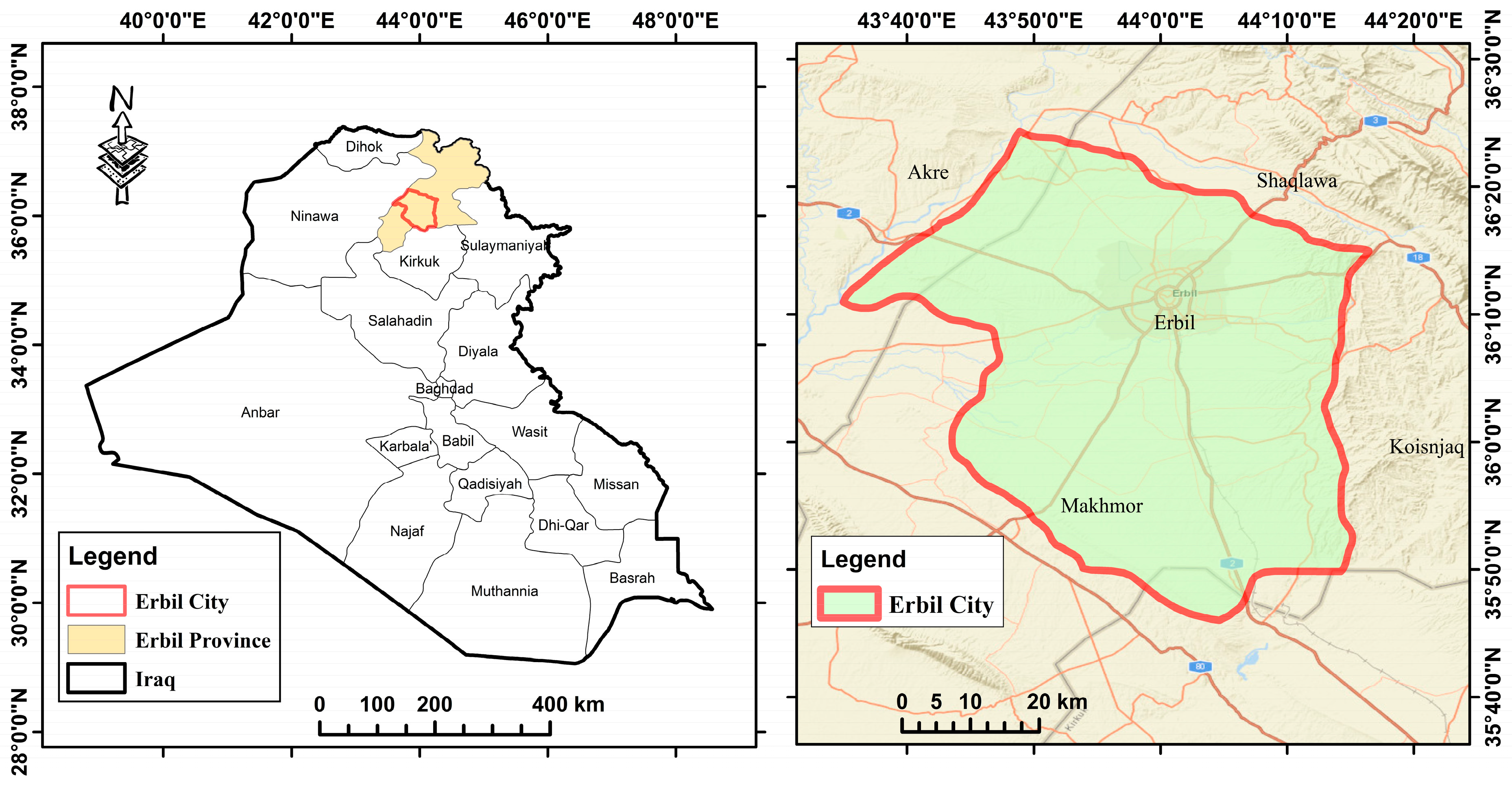
2.1. Description of the Study Area

Erbil, located in northern Iraq, serves as the focus of this study. Its geographic coordinates are 36°11′28″ N and 44°0′33″ E, as illustrated in Figure 1. The region features a broad plain, interspersed with hills to the east that reach elevations up to 426 m above sea level [58]. The landscape is predominantly covered by Quaternary sediments that have accumulated due to the weathering and erosion of the neighboring highlands. Significantly, in the northern and northeastern parts of the study area, the Quaternary sediments lie atop the Bai Hassan formation, composed of molasses-type rock formations. The central section of Erbil is generally flat, whereas the northeastern and eastern areas present a more rugged landscape [59].

Erbil’s climate is classified as semiarid, exhibiting apparent seasonal shifts in humidity. Summers are marked by low humidity, with temperatures often rising above 45 °C, whereas winters experience moderate humidity, with temperatures frequently falling below 0 °C. The area encounters a cool and wet climate, receiving over 400 mm of average annual precipitation [60]. Rainfall usually starts in mid-October and lasts until May.

On 17 December 2021, Erbil and the Kurdistan Region of Iraq faced an unusually severe rainfall following one of the driest years in recent history [61]. Starting at 4 a.m., the rain led to extensive flooding in several districts of Erbil, such as Dara Too, Qush Tappa, Shamamk, Zhyan, Roshinbiri, and Bahrka, especially in the northern and eastern areas of the city. This heavy downpour caused substantial destruction, damaging homes, buildings, and vehicles, and tragically resulting in loss of life [62].

2.2. Flood Detection Datasets

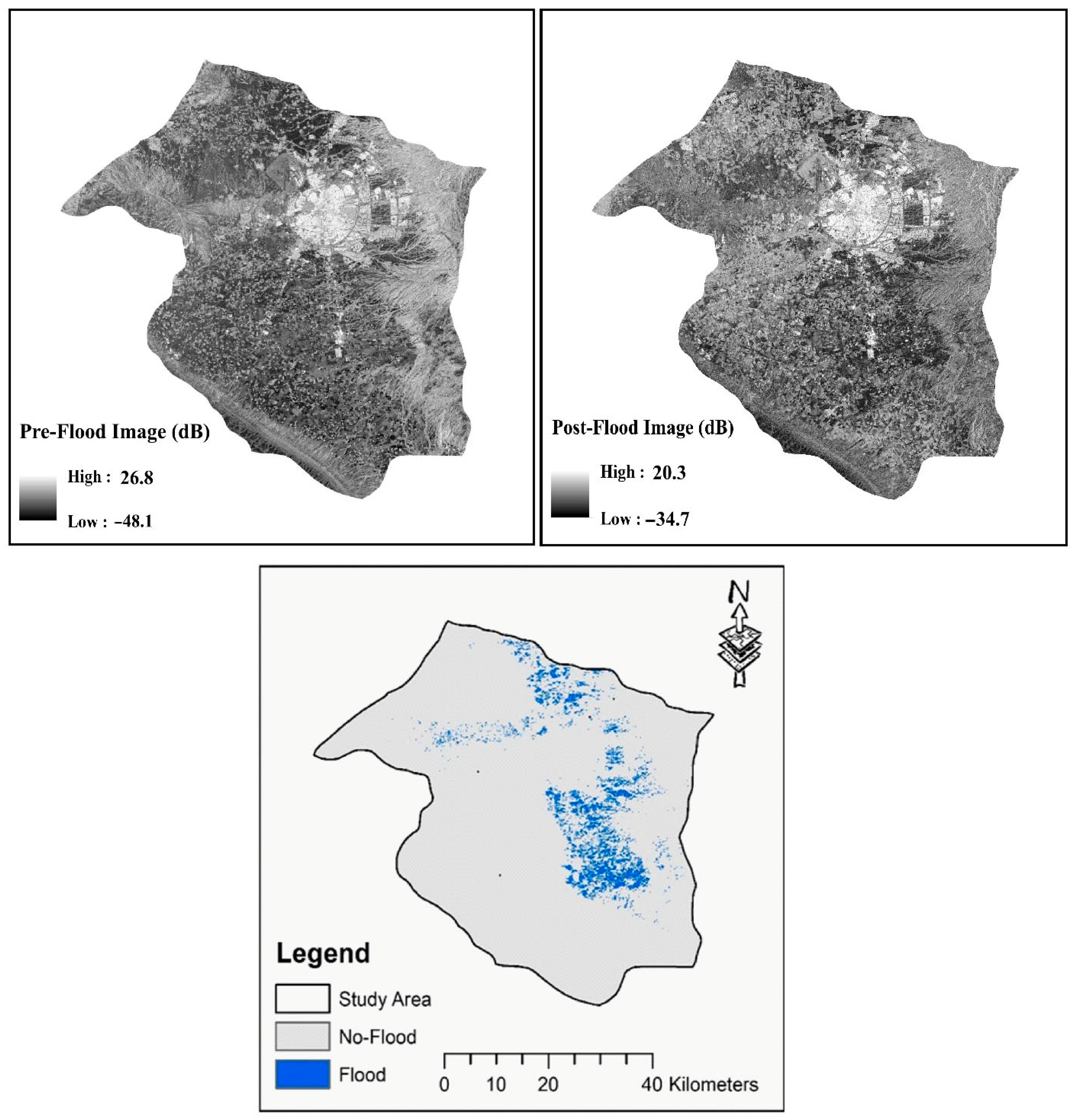
2.2.1. Erbil Flood Dataset

The satellite images from the Sentinel-1 mission were employed in the current research for flood delineation. Based on the Copernicus program of the European Space Agency, the Sentinel-1 offers high-resolution SAR images and includes the possibility of using it for flood monitoring. Differing from the optical images, SAR is insensitive to cloud or illumination, and is suitable for the long-period monitoring of the flood [63]. The study location is Erbil City due to a flash flood that hit the city in December 2021, which resulted in remarkable losses in lives and properties. In the present study, the flood-impinged land surface alteration maps were obtained from the pre-and post-flood SAR scenes (Figure 2). These images were sourced through Google Earth Engine (GEE), a cloud computing platform that specializes in processing geospatial data sets [64], privacy-enabled remote-sensing imagery processing, and analysis at scale using Google Earth Engine.

Table 1. Satellite data from Sentinel-1 used for flood analysis.

Satellite	Acquisition Date	Processing Level	Polarization	Spatial Resolution (m)
Sentinel-1	Pre-flood 25 September 2021	Level 1	Single—VH	10
Sentinel-1	Post-flood 20 December 2021	Level 1	Single—VH	10

presents a summary of the pre- and post-flood preparation process for Sentinel-1 images for assessing the impact of the flash flood. The acquisitions of data were collected in the Interferometric Wide Swath (IW) beam mode, which provides a wide swath at medium resolution and is considered appropriate for large-scale disaster monitoring. The high-resolution (HR) data (10 m × 10 m spatial resolution) can ensure the precision monitoring of waters, land sinks, and infrastructure damages. This method, with a swath-width of 250 km per swath, can scale large regions with a flooding disaster.

The raw radar data from Sentinel-1 goes through a preprocessing phase, which involves standard procedures to prepare for further analysis. The first step is processing this raw data, including radiometric calibration to adjust for sensor and atmospheric influences, ensuring that the signal strength accurately reflects surface characteristics. Afterward, geometric correction aligns the data with the Earth’s surface, compensating for distortions caused by the satellite’s movement and the curvature of the Earth. Speckle filtering is applied to reduce noise from the radar signal interacting with the surface, enhancing the visibility of features such as bodies of water or buildings. Speckle noise commonly affects SAR images, complicating visual analysis. Lee (5 × 5) speckle filtering is implemented to mitigate this noise while preserving image details. Additionally, orthorectification corrects distortions caused by terrain variations, ensuring that the resulting images accurately represent the Earth’s surface. The data may also be subsetted based on specific use cases, such as masking flooded areas for targeted data analysis by researchers. This preprocessing is crucial for improving the quality and applicability of satellite data in monitoring events like flash floods. All preprocessing steps of the Sentinel-1 dataset were implemented using JavaScript in GEE.

2.2.2. S1GFloods Dataset

The benchmarking data of our model consists of the data in Reference [16], which used the Sentinel-1 SAR database satellite images. This radar imaging system, designed by the European Space Agency (ESA), can create high-resolution images regardless of weather, time of day, or atmosphere opacity. The dataset covers common and high-impact causes of flooding, such as heavy rainfall, riverine flooding, dams and levee failure, tropical storms, and hurricanes. Its geographic variation ensures the adaptability of the flood monitoring method to a wide range of environmental scenarios, such as rural, mountainous, urban communities, vegetated zones, rivers, ponds, lakes, and reservoirs.

The dataset contains 4830 image sets consisting of pre-flood, post-flood, and change-labeled images. Each image is of size 256 × 256 pixels and has 3 channels that represent the Red (R), Green (G), and Blue (B) in RGB images. The labels are provided as a single channel; each pixel is assigned as flood (0) or non-flood (1). In order to better train the flood detection model, the dataset is divided into a training set, which has 4300 image sets (90% in total), and a test set, which consists of 530 image sets (10% in total). Training sets are further divided into two smaller training subsets and a validation subset to train the model with the right parameters. A model that has this division allows a good generalization that reduces the chance of overfitting and enhances learning.

3. Methodology

3.1. Network Architecture Overview

This research introduced the Compact Convolutional Tokenizer-based Hybrid U-Net and Vision Transformer Model (CCT-U-ViT) (Figure 3). This innovative model features a hybrid architecture designed for Synthetic Aperture Radar (SAR)-based flood detection, integrating U-Net’s spatial feature extraction with the Transformer’s global context modeling. The system processes pre- and post-flood SAR images utilizing a U-Net encoder–decoder framework with skip connections; the encoder methodically extracts hierarchical features using 8, 16, 32, and 64 filters across four levels. Each encoder level corresponds to a decoder layer, facilitating the reconstruction of spatial details. At the bottleneck layer, equipped with 128 filters, the model employs three vital enhancement modules: a Compact Convolutional Transformer (CCT) tokenizer that transforms 2D pooled features into 1D tokens for sequential processing, position embedding for adding spatial awareness (a dense 128-dimensional structure), and transformer blocks that implement multihead attention mechanisms along with MLP and skip connections to capture long-range dependencies. The U-Net’s spatial features are merged with the global features derived from the transformer via a feature fusion module, which concatenates, densifies (to 64 channels), and applies a dropout rate of 0.2 for regularization. Ultimately, a binary classification head with dense layers differentiates between flood and non-flood pixels, enabling the model to utilize local spatial patterns through the U-Net path and global contextual relationships via the transformer path to delineate flood boundaries precisely.

3.2. U-Net Architecture

The U-Net module utilizes an encoder–decoder architecture frequently used in segmentation tasks. The encoder path extracts hierarchical features from the input image, while the decoder reconstructs the image or generates high-level representations. Comprising multiple blocks, the encoder contains convolutional layers, which are followed by batch normalization and ReLU activation. As the blocks progress, they reduce the spatial resolution of the feature maps, capturing more abstract representations. At the end of each encoder block, max-pooling layers downsample the feature maps. Conversely, the decoder path employs transposed convolutions to enhance the resolution of feature maps, along with concatenation with corresponding encoder features via skip connections. This methodology enables the model to utilize fine-grained spatial information from earlier layers, improving prediction accuracy. In both the encoder and decoder paths, each convolutional block features two convolutional layers with 3 × 3 kernels, followed by batch normalization and ReLU activation. Ultimately, the U-Net decoder path produces a high-level feature representation of the input image.

3.2.1. U-Net Encoder with Hierarchical Convolutional Blocks

The encoder path comprises a series of convolutional blocks, each containing convolutional layers that utilize batch normalization and ReLU activation (Figure 4). As these blocks proceed, they incrementally increase the filter count while decreasing spatial dimensions using max-pooling, which helps extract increasingly abstract hierarchical features. Skip connections from each encoder stage preserve high-resolution spatial details for subsequent reconstruction.

The encoder uses convolutional layers to extract features. The general form of the convolution operation is:

$$F\_out=sigmoid\left(W\ast X+b\right)$$

(1)

where: F_out is the output feature map, $W$ is the convolution filter (kernel), $X$ is the input feature map, $b$ is the bias term, $\mathsf{\sigma }$ represents the activation function (ReLU).

Max pooling reduces spatial resolution:

$$X\_pooled=\mathit{max}\_\mathit{pooling}\left(X,f\right)$$

(2)

where $f$ is the filter size.

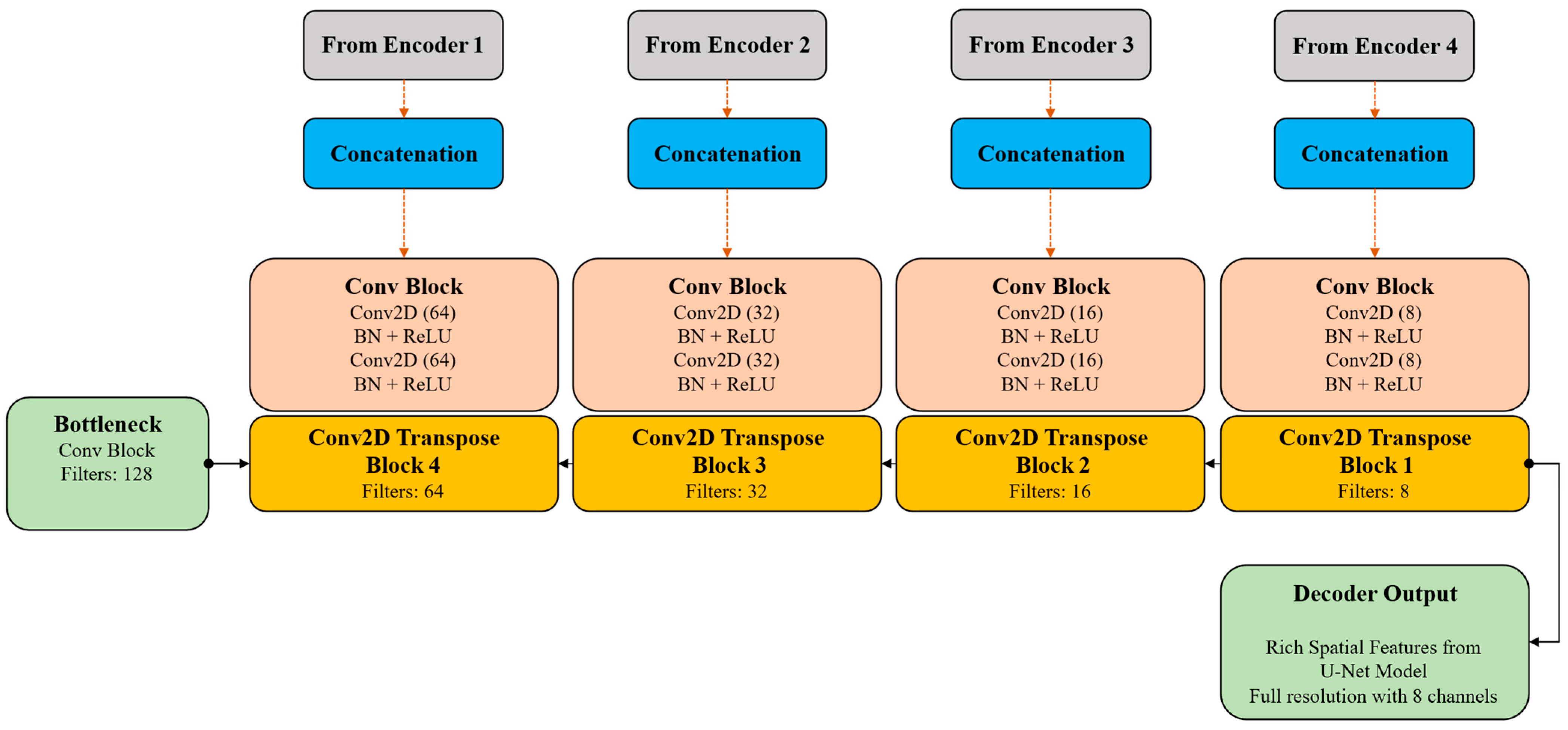
3.2.2. U-Net Decoder with Transposed Convolutions and Skip Connections

The decoder reflects the encoder’s architecture but uses transposed convolutional layers for upsampling (Figure 5). In every decoder phase, features from the related encoder block are concatenated via skip connections, restoring fine-grained spatial details diminished during downsampling. Additional convolutional blocks enhance the upsampled feature maps, leading to better spatial reconstruction.

The decoder uses transposed convolutions to upsample the feature maps. The formula for the transposed convolution is:

$$F\_out\_prime=sigmoid(np.dot(W\_prime, X\_prime)+b\_prime)$$

(3)

where $F\_out\_prime$ is the output feature map after upsampling, $W\_prime$ is the transposed convolution filter, $X\_prime$ is the input feature map, $b\_prime$ is the bias term, sigmoid represents the activation function (ReLU).

3.3. CNN-Based Tokenizer for Transformer Input (CCTTokenizer)

Rather than employing standard patch extraction, the transformer branch uses a CNN-based tokenizer. This approach yields richer and more informative tokens by learning spatial features before sending sequences into the transformer, thus improving the quality of tokens for subsequent attention mechanisms. The CCTTokenizer layer acts as the CNN tokenizer, converting the image into a sequence of patches through a succession of convolutional and pooling layers. Initially, the convolutional layers, which use 3 × 3 kernels, capture low-level features, followed by max-pooling layers that decrease spatial dimensions. Finally, the output from this segment is reshaped into a sequence of tokens for processing by the Transformer. The architecture of this module is presented in Figure 6.

The CCT tokenizer performs convolution followed by max-pooling:

$$X\_prime=\mathit{conv}2d\left(X,W,f\right) \mathit{and} X\_prime=\mathit{maxpooling}2d\left(X\_prime,f\right)$$

(4)

where $f$ represents the filter size.

Spatial information is integrated into the tokenized patches by applying positional embeddings to the CNN tokenizer’s output. These embeddings are trained and then merged with the tokenized patches. This allows the Transformer to understand the relative positions of patches in the image.

The composite raster image (pre- and post-flood) is divided into 2D image patches. These patches are passed through two Conv2D and Pooling layers to learn the spatial and semantic features of the image data. After feature extraction, the resulting feature maps are flattened into 1D feature vectors. To preserve the spatial relationships of these features, positional embeddings are applied. This allows the integration of the learned feature vectors from the Conv2D/Pooling layers with positional vectors, resulting in enriched spatial feature vectors that maintain the spatial information across the image.

3.4. Transformer Blocks

The transformer branch includes several encoder layers, each incorporating layer normalization, multihead self-attention with adjustable head counts and projection sizes, and position-wise feedforward MLPs that utilize GELU activations and dropout for regularization (Figure 7). Residual skip connections between the layers improve gradient flow and support stable training. Learned positional embeddings are combined with token embeddings to offer spatial context.

Each Transformer layer incorporates a multihead attention mechanism that operates on the tokenized patches to capture long-range dependencies between image regions. Num_heads specifies the number of attention heads, while the attention space’s dimensionality is indicated by projection_dim. After each attention operation, a residual connection is included in the output to aid training. This is followed by a feedforward neural network that consists of two dense layers utilizing GELU activations and dropout for regularization. Layer normalization is applied after both the attention and feedforward layers to enhance training stability. The Transformer block’s output is improved through multiple layers, enabling the model to capture local and global contextual information.

The transformer block uses multihead attention and a multilayer perceptron (MLP) for feature extraction. The multihead attention operation is defined as:

$$\mathrm{Attention}\left(Q,K,V\right)=softmax\left(\right(Q \ast K^T)/sqrt(d\_k\left)\right) \ast V$$

(5)

where $Q$ is the query matrix, $K$ is the key matrix, $V$ is the value matrix, d_k is the dimension of the key.

The output is fed into an MLP:

$$\mathrm{MLP}\left(X\right)=W1 \ast \mathrm{ReLU}\left(W2 \ast X+b2\right)+b1$$

(6)

where W1, W2, b1, and b2 are learned weights and bias terms.

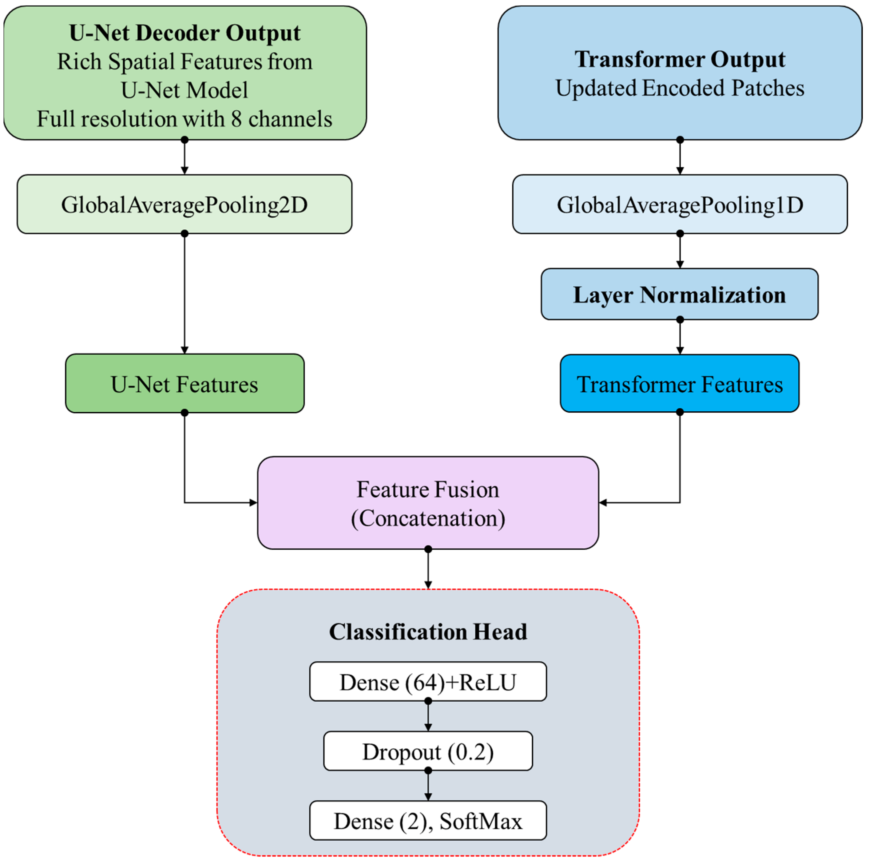
3.5. Feature Fusion and Classification Head

After processing independently, the global average pooled features from the U-Net decoder are concatenated with the transformer outputs to form a detailed feature vector that captures local spatial and global contextual information. The outputs of the U-Net model are 2D local feature maps. The use of GlobalAveragePooling2D computes the average of all the values in each feature map (channel) across both the height and width dimensions. Essentially, it reduces each 2D feature map (spatial grid) to a single scalar value, representing the average of all the values in that feature map. The output is a 2D tensor of shape (batch_size, channels), where each channel has a single average value computed from its corresponding 2D spatial grid. On the other hand, the Transformer outputs are 1D global feature sequences. The use of GlobalAveragePooling1D computes the average of all the values along the sequential dimension, resulting in a single value for each channel. The output is a 2D tensor of shape (batch_size, channels), where each channel contains the average of the values along the steps dimension. The fusion of the local features from U-Net and the global features from Transformer is then concatenated into single feature vectors, which are used for the classification layer.

This combined vector is passed through fully connected layers with dropout regularization and ReLU activation, leading to a final dense layer that yields logits for binary classification. A fully connected layer featuring 64 units and ReLU activation is applied to this integrated feature vector. To avoid overfitting, dropout regularization is incorporated with a dropout rate of 0.2. Ultimately, the final output is produced by a dense layer with two units (representing binary classification) and no activation function, intended for use with a binary cross-entropy loss function. Figure 8 presents this feature fusion and classification head module.

Feature fusion concatenates features from the U-Net and Transformer branches:

$$F\_fused=[F\_U-Net+F\_Transformer]$$

(7)

where F_U-Net and F_Transformer are the features from the U-Net and Transformer branches, respectively. The classification head computes the final output:

$$y=softmax(W\_class \ast F\_fused+b\_class)$$

(8)

where W_class is the weight matrix for classification, and b_class is the bias term for classification.

3.6. Benchmark Models

3.6.1. CNN 2D-1 Layer [21]

This model employs a sequential Convolutional Neural Network architecture, starting with a 2D convolutional layer with 32 filters and a 2 × 2-pixel kernel size. It uses Rectified Linear Unit (ReLU) activation to introduce non-linearity, processing input tensors of shape (3, 3, 2). The feature maps are then flattened into a one-dimensional vector, connecting to a fully connected layer with 16 hidden units that also use ReLU activation. The network ends with a dense layer of 2 units, applying Softmax activation to generate probability distributions for target classes. This design allows the network to capture hierarchical features through convolution while keeping a lightweight parameter count due to its limited filters and hidden units.

3.6.2. CNN 2D-2 Layers [21]

This model is a sequential Convolutional Neural Network with two layers. The first layer has 64 filters and a 2 × 2 kernel size, using ReLU activation on input tensors of shape (3, 3, 2). The second layer comprises 32 filters and a 1 × 1 kernel with ReLU activation. This architecture allows for hierarchical feature extraction, as the first layer captures local patterns while the second refines features. After the convolutional layers, feature maps are flattened into a one-dimensional vector and processed through a fully connected layer with 16 hidden units and ReLU activation. The network concludes with a dense output layer featuring two units and Softmax activation for probability distributions across target classes.

3.6.3. CNN 3D-1 Layer [65]

The 3DCNN model is based on 3D Convolutional Neural Networks, taking (3,3,2) as input tensor size and expanded to (3, 3, 2, 1) with the 3D Convolutional Neural Network that can handle batch, spatial input data. It begins with a 3D version of a convolutional layer, containing 32 2 × 2 × 1-pixel filters to perform 2D convolutions through the input channels while preserving channel dimension. However, non-linearity is introduced with ReLU activation functions. The output is a feature map set reshaped to a 1D-vector that flows through a fully connected layer with 16 ReLU hidden units. The network also has a final dense output layer with 2 units and Softmax activation that provides probability distributions of the target classes.

3.6.4. CNN 3D-2 Layers [22]

The model is built on the Keras framework and utilizes a two-layer 3D Convolutional Neural Network. It takes a tensor input with size [p × p × channels] and produces a reshaped output of size [p × p × channels × 1]. The first layer has 64 2 × 2 × 1 pixel kernel filters, and the second layer has 32 2 × 2 × 1 pixel kernel filters; both layers use ReLU activation. In this structure, the hierarchical feature extraction process is enabled, and at the same time, the channel dimension is preserved. The feature maps from the second layer are flattened to form a 1D vector, which is fed into a fully connected layer of 16 hidden units with ReLU activation. The network is topped off with a dense output layer having [output_shape] nodes with Softmax activation, used to generate probabilities across all the target classes.

3.6.5. Hybrid CNN [66]

Model architecture: Our model uses a hybrid CNN (both 3D and 2D convolutions) following the Keras functional API. Input tensors of dimensions [p × p × channels] are reshaped to [p × p × channels × 1]. It is composed of two 3D convolutional layers, the first with 64 filters (kernel size 3 × 3 × 2) and the second with 32 filters (kernel size 3 × 3 × 1), all using ReLU activation. After these layers, feature maps are reshaped into a single dimension by combining the dimensions of filter and feature-map channels along which we will perform 2D convolutions. A 2D convolutional layer using 16 filters (3 × 3 kernel size) and the rectified linear activation is then applied. This architecture is designed such that the network can learn spatiotemporal patterns through 3D convolutions and treat fused features using 2D convolutions. Finally, the feature maps are flattened to a one-dimensional vector and go through a fully connected layer with 16 hidden units and ReLU activation. A dropout layer with a 0.5 rate for dropout is used to avoid overfitting before the output layer, which has [output_shape] units with Softmax activation, and returns the probability values of classes.

3.6.6. U-Net [67]

The model architecture uses a modified U-Net CNN with an encoder–decoder structure and skip connections via the Keras functional API. It has three components: the encoder path, a bottleneck, and a decoder path, each using specialized convolutional blocks. However, these blocks perform a 3 × 3 convolution followed by batch normalization, ReLU activation, and a 1 × 1 convolution with the same normalization and activation. This dual-convolution technique supports spatial feature extraction and channel refinement. The encoder path comprises four blocks, combining a convolutional block with 1 × 1 max pooling, with filter counts increasing (8, 16, 32, 64) for hierarchical feature extraction. Each encoder block retains features before pooling through skip connections for the decoder. The bottleneck contains a convolutional block with 128 filters, linking the encoder and decoder while managing abstract features. The decoder mirrors the encoder with four blocks, starting with a 1 × 1 transposed convolution (upsampling) and concatenating corresponding skip features, merging low-level spatial data with high-level semantics. Filter counts decrease (64, 32, 16, 8), reconstructing spatial resolution and reducing feature complexity. After the decoder, global average pooling condenses dimensions to 1 × 1, summarizing information across the feature map. The network ends with a dense output layer with [output_shape] units and sigmoid activation for binary classification.

3.6.7. Vision Transformer (ViT) [43]

The ViT model is a patch-based technique that processes input tensors, utilizing a transformer architecture for feature extraction and classification. The patches layer segments the input image (3 × 3) into non-overlapping 1 × 1 patches, which are projected into a higher-dimensional space (projection_dim = 64) via the PatchEncoder layer with learnable position embeddings. The transformer backbone includes four layers with: a multihead self-attention mechanism (4 heads), layer normalization (epsilon = 1 × 10⁻⁶) with residual connections, and a multilayer perceptron (MLP) with GELU activation, consisting of two dense layers sized [64, 128] and a dropout rate of 0.1. Following the transformer layers, the architecture normalizes the final encoded representation, flattens spatial dimensions, applies dropout regularization at 0.5, and includes a final MLP head with two dense layers sized [32, 64] and a dropout rate of 0.5, finishing with an output layer using Softmax activation for classification. The model uses the Adam optimizer with a learning rate of 0.001 and weight decay of 0.0001. Binary cross-entropy is the loss function, and performance is evaluated using binary accuracy metrics. Data are processed in batches of 32 samples.

This Vision Transformer architecture preserves the original ViT principles, tailored for smaller images by adjusting patch sizes and hyperparameters. Dropout regularization (0.1 in transformer layers and 0.5 in final layers) and layer normalization mitigate overfitting, while multihead attention helps the model understand complex spatial relationships.

3.6.8. CNN–Transformer [68]

The model’s architecture integrates a hybrid Convolutional Neural Network (CNN) with a Transformer framework, optimized for effective visual data processing. Initially, input images are processed through a custom CCTTokenizer layer that performs convolutional operations and pooling to extract spatial features, reshaping the data into token sequences that the transformer can process. Positional embeddings can be included to represent the spatial relationships among the image patches. The model’s core comprises stacked transformer layers equipped with multihead self-attention, layer normalization, stochastic depth for regularization, and a feedforward network. Following the transformer layers, a SequencePooling layer utilizes soft attention on the token sequences to generate a pooled representation, which is forwarded to a fully connected output layer to facilitate either classification or regression. Various regularization techniques, such as dropout and stochastic depth, are implemented to reduce overfitting, while the model is optimized using binary cross-entropy loss and label smoothing for classification purposes.

3.7. Performance Metrics

A set of common evaluation metrics is adopted to evaluate the performance of deep-learning models according to their accuracy in detecting floods in SAR images. We calculate these measures to investigate how well the model distinguishes between the flood and non-flood pixels. The performance measures used in this study are:

Accuracy measures the proportion of correctly classified pixels, including flood and non-flood categories, compared to the total pixel count in the dataset. It is defined as:

$$Accuracy=(TP+TN)/(TP+TN+FP+FN)$$

(9)

where:

• TP = True Positives (correctly detected flood pixels)
• TN = True Negatives (correctly detected non-flood pixels)
• FP = False Positives (non-flood pixels classified as flood)
• FN = False Negatives (flood pixels classified as non-flood)

Cohen’s Kappa coefficient evaluates the alignment between predicted and actual classifications, factoring in chance agreement. Its calculation is as follows:

$$\kappa =(P_o-P_e)/(1-P_e)$$

(10)

where:

• $P_o$ = Observed agreement (the actual accuracy of the model)
• $P_e$ = Expected agreement by chance (the agreement expected if the model were to classify randomly)

A higher Kappa value signifies improved agreement beyond what would be anticipated by chance.

The F1 Score represents the harmonic mean of precision and recall. This metric is particularly valuable for handling imbalanced datasets because it balances the trade-off between false positives and false negatives:

$$F1=(2\times Precision\times Recall)/(Precision+Recall)=\left(2TP\right)/(2TP+FP+FN)$$

(11)

where:

• Precision is the proportion of detected flood pixels that are correctly classified as flood
• Recall is the proportion of actual flood pixels that are correctly detected

The mean Intersection-over-Union (mIoU) metric measures the overlap between predicted and actual flood areas. It represents the average Intersection over Union for both flood and non-flood classes:

$$\mathrm{mIoU}=0.5 \ast \left(\left(\right(TP/(TP+FP+FN))+((TN/(TN+FN+FP)\right))$$

(12)

This metric evaluates the model’s ability to correctly distinguish between flood and non-flood areas by determining the ratio of the intersection of predicted and actual regions to their union.

4. Results and Discussions

4.1. Experimental Setup and Parameter Settings

The trials were performed on a high-performance computing workstation equipped with an Intel architecture CPU including 24 physical and 32 logical cores, together with 32 GB of RAM, which exhibited a 69.0% usage during training. However, the NVIDIA GeForce RTX 4070 Ti GPU enhanced this system’s computing power, providing 28.3 GB of VRAM and facilitating mixed-precision training with the Ampere architecture, essential for managing large flood detection datasets and complex model architectures. Furthermore, the deep-learning framework was developed with Python 3.10, utilizing TensorFlow 2.9.1 and the Keras API, chosen for its efficiency in GPU resource utilization and suitability for computer vision applications. The model’s architecture employed Sentinel-1 SAR images, utilizing 3 × 3 spatial patches to facilitate temporal comparisons of circumstances pre- and post-flood, hence enabling flood detection via a binary classification approach.

For training, the Adam optimizer was employed with standard adaptive learning rates and key parameters set as Beta1 = 0.9, Beta2 = 0.999, and Epsilon = 1 × 10⁻⁷, which aids in achieving stable convergence even amid noisy data. We selected the binary cross-entropy loss function to ensure appropriate gradient signals for binary classification tasks. The dataset contained 54,733,367 labeled pixels, highlighting a significant class imbalance (with a 1:31 ratio of flood to non-flood pixels) and was split into 70% for training, 10% for validation, and 20% for testing. Data preprocessing involved normalizing pixel values and extracting 3 × 3 patches from co-registered SAR imagery, explicitly avoiding data augmentation to preserve the integrity of radar backscatter characteristics. The model underwent training for 100 epochs with a batch size of 64, and it was evaluated using various metrics, including overall accuracy (OA), Kappa coefficient, F1-score, and mean Intersection over Union (mIoU), to ensure a comprehensive performance assessment despite the existing class imbalance. Additionally, memory management techniques were implemented to optimize GPU memory usage, with batch processing tailored for the RTX 4070 Ti, and random seed initialization was performed to ensure the reproducibility of results.

$$bce\_loss(x,y)=-1 \ast (y \ast math.log(x)+(1-y) \ast math.log(1-x\left)\right)$$

(13)

4.2. Results of Erbil Flood Detection

The evaluation results in

Table 2. Accuracy assessment of the proposed and benchmark models for flood detection on the Erbil dataset.

Model	Metric
	OA	Kappa	F1 Score	mIoU
CNN 2D-1 Layer	0.9041	0.8082	0.9031	0.8234
CNN 2D-2 Layers	0.9056	0.8113	0.9044	0.8254
CNN 3D-1 Layer	0.8741	0.7482	0.8642	0.7609
CNN 3D-2 Layers	0.8892	0.7784	0.8845	0.7929
Hybrid CNN	0.9008	0.8016	0.8985	0.8158
U-Net	0.8953	0.7907	0.9013	0.8204
ViT	0.9064	0.8127	0.9086	0.8326
CNN–Transformer	0.9079	0.8158	0.9076	0.8308
CCT-U-ViT (ours)	0.9124	0.8248	0.9121	0.8383

highlight the superior performance of the proposed CCT-U-ViT architecture across all established evaluation metrics, providing empirical support for the model’s effectiveness in flood detection tasks. The CCT-U-ViT model attained the highest overall accuracy (OA) of 91.24%, marking a 1.45% increase over the second-best model, CNN–Transformer, which scored 90.79%. This improvement holds significant practical relevance due to the extensive scope of satellite imagery analysis. The performance boost is attributed to the effective integration of convolutional compact transformers with the U-Net architecture, allowing the model to capture local spatial dependencies through convolutional operations and long-range contextual relationships using self-attention mechanisms. With a Kappa coefficient of 0.8248, the CCT-U-ViT demonstrates excellent inter-rater reliability. Its performance greatly surpasses chance agreement, showcasing a statistically significant improvement over baseline methods for flood detection applications.

The comparative analysis reveals apparent performance differences among various architectural paradigms. Traditional 2D CNN methods (90.41–90.56% OA) perform well due to their ability to harness spatial correlations and the translation invariance properties inherent in satellite imagery. On the other hand, 3D CNN models show comparatively lower performance (87.41–88.92% OA) because of their increased complexity and the risk of overfitting when temporal dimensions are added without sufficient training data. The ViT achieves competitive results (90.64% OA) by utilizing global attention mechanisms, but the quadratic computational complexity of self-attention and limited inductive biases for spatial data hinders its performance. The U-Net architecture (89.53% OA), effective for general segmentation tasks thanks to its encoder–decoder structure with skip connections, also encounters challenges in addressing the spectral complexity and spatial variability often seen in flood detection scenarios. These insights are further corroborated by the F1-score and mIoU metrics, with CCT-U-ViT achieving 0.9121 and 0.8383, respectively, reflecting a superior balance of precision and recall, as well as Intersection-over-Union performance, which are critical for accurately defining flood boundaries.

The qualitative assessment of flood detection results in Figure 9 and Figure 10 highlights differences in spatial pattern recognition abilities among the architectures evaluated, affecting operational flood monitoring applications. The ground truth reference (Figure 9c) displays intricate flood patterns with irregular boundaries and fragmented water bodies throughout the study area, posing significant challenges for automated detection algorithms. Visual analysis reveals that CCT-U-ViT generates the most spatially coherent flood maps with excellent boundary preservation, thanks to the hierarchical feature extraction capabilities of the Compact Convolutional Transformer and the multiscale representation learning of the U-Net decoder pathway.

Transformer-based models, such as ViT, CNN–Transformer, and CCT-U-ViT, preserve flood boundary integrity and minimize salt-and-pepper noise artifacts frequently observed in pixel-wise classification methods. This improvement is due to the self-attention mechanism, which effectively captures long-range spatial dependencies and contextual relationships, facilitating superior differentiation between spectrally similar but spatially distinct land cover types. In contrast, traditional CNN architectures face challenges with fine-scale boundary details; 2D CNNs tend to produce excessively smoothed boundaries attributable to successive pooling operations, while 3D CNNs demonstrate significant fragmentation, likely stemming from difficulties in learning optimal spatiotemporal filters with limited training data.

The U-Net architecture demonstrates moderate performance and exhibits typical encoder–decoder artifacts. This includes occasional missed detections in smaller flooded areas and minor over-segmentation in transition zones. Such behavior is consistent with U-Net’s optimization for biomedical image segmentation, where its skip connections, while preserving spatial resolution, may struggle with the spectral complexity and radiometric variations found in multispectral satellite imagery. The superior capabilities of attention-based models—especially in sustaining spatial coherence—highlight the advantages of explicitly modeling spatial relationships through attention mechanisms, compared to purely convolutional methods in complex Earth-observation tasks.

The detailed error analysis presented in Figure 10 provides essential insights into the modes of model failure and their root physical and methodological causes. In addition, Figure 11 provides zoomed areas of the most significant differences among the prediction maps. The patterns of error distribution highlight consistent biases linked to key difficulties in satellite-based flood detection, such as spectral confusion, mixed pixel effects, and atmospheric interference. False positive detections, illustrated in yellow, mainly occur in regions with high soil moisture, shadows from topography, and permanent water bodies that closely resemble the spectral signatures of floodwaters. These errors are particularly evident in 3D CNN models, suggesting that including the temporal dimension, despite its theoretical benefits, may introduce noise when training data lacks adequate temporal diversity or when atmospheric conditions differ significantly between acquisition dates.

False negative detections (shown in magenta) primarily occur in shallow flood zones and vegetated wetlands, where emergent vegetation or sediment load weakens the water signal. The lower false negative rates in transformer-based models are attributed to their superior capacity to capture contextual details and subtle spectral changes via global attention mechanisms. The CCT-U-ViT model exhibits the most balanced error distribution, featuring significantly reduced false positive rates (indicating enhanced precision) while maintaining high sensitivity for actual flood detection. This indicates that the hybrid architecture effectively integrates the spatial inductive biases of CNNs with the contextual modeling strengths of transformers.

4.3. Experimental Results on the S1GFloods Dataset

The thorough assessment of the S1GFloods benchmark dataset reveals the outstanding performance of the CCT-U-ViT architecture, achieving leading results in all evaluation metrics and setting new benchmarks for satellite-based flood detection (

Table 3. Accuracy assessment of the proposed and benchmark models for flood detection on the S1GFloods dataset.

Method	Kappa	OA	F1 Score	mIoU
CNN 2D-1 Layer	0.872	0.937	0.911	0.843
CNN 2D-2 Layers	0.908	0.956	0.933	0.877
CNN 3D-1 Layer	0.911	0.959	0.937	0.882
U-Net	0.927	0.955	0.932	0.877
CNN 3D-2 Layers	0.930	0.955	0.932	0.878
ViT	0.945	0.961	0.941	0.896
Hybrid CNN	0.936	0.962	0.942	0.894
CNN–Transformer	0.958	0.968	0.952	0.915
CCT-U-ViT (ours)	0.969	0.979	0.966	0.933

). This model reached a top overall accuracy of 97.9%, marking a noteworthy 1.1% improvement over the second-best method (CNN–Transformer at 96.8%), a considerable leap given the already impressive baseline performance on this challenging dataset. The Kappa coefficient 0.969 suggests near-perfect agreement beyond mere chance, underscoring the model’s exceptional reliability for operational flood monitoring applications.

The performance hierarchy identified in the S1GFloods dataset provides important insights into architectural design principles for flood detection tasks. Traditional CNN methods display a distinct performance gradient, with deeper architectures (CNN 2D-2 Layers: 95.6% OA) surpassing their shallower versions (CNN 2D-1 Layer: 93.7% OA) due to better feature abstraction capabilities and broader receptive field coverage. 3D CNN architectures demonstrate competitive performance (95.9% OA for a single layer, 95.5% OA for two layers), suggesting that the temporal dimension offers valuable information when ample training data are available, as evident with the extensive S1GFloods benchmark. The Vision Transformer achieved excellent results (96.1% OA, 0.945 Kappa) by utilizing global attention mechanisms, although its computational complexity poses a practical challenge for large-scale use.

The CNN–Transformer hybrid approach (96.8% OA, 0.958 Kappa) demonstrates the effectiveness of combining convolutional inductive biases with transformer attention mechanisms, achieving superior performance compared to pure CNN or transformer architectures. However, the proposed CCT-U-ViT surpasses all baseline methods with an F1-score of 0.966 and mIoU of 0.933, indicating exceptional precision-recall balance and spatial overlap accuracy. The consistent performance gains across all metrics (2.1% improvement in Kappa, 1.1% in OA, 1.4% in F1-score, and 1.8% in mIoU compared to the second-best method) provide strong empirical evidence for the architectural innovations incorporated in the CCT-U-ViT design, particularly the effective integration of multiscale feature fusion with hierarchical attention mechanisms optimized for satellite imagery analysis.

4.4. Comparison of Computational Efficiency

The assessment of computational efficiency reveals trade-offs between model complexity and performance, affecting deployment in resource-limited settings (

Table 4. Comparison of computational efficiency of the proposed and baseline models for flood detection based on the Erbil dataset.

Model	# Layers	# Parameters	Trainable Parameters	Model Size (MB)	Inference Time (Batch 64) (s)	Batch Time (Batch 64) (s)
CNN 2D-1 Layer	4	2386	2386	0.03	0.0232	634.62
CNN 2D-2 Layers	5	4754	4754	0.04	0.0181	495.86
CNN 3D-1 Layer	4	4306	4306	0.03	0.0218	595.25
CNN 3D-2 Layers	5	9618	9618	0.06	0.0183	501.54
CNN–Transformer	29	407,683	407,683	1.64	0.0231	632.13
Hybrid CNN	9	4130	4130	0.04	0.02	545.8
U-Net	69	237,946	236,474	1.12	0.0233	638.21
CCT-U-ViT	95	669,482	668,010	2.82	0.0258	705.91
ViT	47	372,770	372,770	1.57	0.0383	1047.76

). Conventional CNN architectures show excellent efficiency, with the 2D single-layer model needing only 2386 parameters (0.03 MB) and achieving an inference time of 0.0181 s per batch. The 3D CNN variants have a slight increase in parameters (4306–9618) while maintaining competitive inference speeds, demonstrating effective use of the temporal dimension. However, this efficiency correlates with lower accuracy compared to attention-based methods.

Transformer-based architectures require more computation, with ViT needing 372,770 parameters (1.57 MB) and the slowest inference time at 0.0383 s per batch, highlighting the quadratic complexity of self-attention. In contrast, the CNN–Transformer hybrid balances performance, having 407,683 parameters (1.64 MB) and faster inference (0.0231 s) than pure ViT, illustrating the benefits of convolutional inductive biases. U-Net shows moderate complexity with 237,946 parameters (1.12 MB) and competitive speed (0.0233 s), making it suitable for accuracy and efficiency. The CCT-U-ViT is the most complex architecture, with 669,482 parameters (2.82 MB) and an inference time of 0.0258 s per batch, positioned between pure transformers and hybrids in computational cost. Despite its size, CCT-U-ViT offers an excellent accuracy-efficiency balance, with only an 11% slower time than the fastest transformer method (CNN–Transformer), achieving greater accuracy. The parameter-to-performance ratio indicates CCT-U-ViT gains a 0.145% accuracy enhancement per additional 1000 parameters compared to CNN–Transformer, demonstrating effective model capacity use for flood detection. Operationally, the model’s 2.82 MB size is feasible for modern systems, and its sub-second inference allows real-time processing of satellite imagery for emergency response.

5. Conclusions

This study successfully used a new hybrid deep-learning model for flood detection using Synthetic Aperture Radar (SAR) imagery, combining the latest advanced techniques, including CNN, U-Net, and Transformer. The primary aim was to evaluate the accuracy and suitability of these models in recognizing flood inundation areas under challenging conditions. The proposed model, by leveraging the VH Sentinel-1 image data, showed excellent performance in flood detection as compared with several benchmark models. In particular, Transformer and hybrid models achieved better performance compared to the U-Net and CNN (2D or 3D) models. The models also achieved comparable results on a test dataset (S1GFloods), further indicating the high performance in detecting flood zones in SAR images.

Integration of these models in operational flood monitoring systems would substantially advance the detection of floods in terms of speed and accuracy by providing instant and timely information for disaster management. These models, by utilizing near-real-time imagery data, can support disaster response efforts, especially when on-ground information is scarce. The results of this study demonstrate the importance of SAR data for advanced deep-learning-based flood response and preparedness, particularly with respect to such flood-prone areas where traditional infrastructure for flood detection is limited.

Nevertheless, several issues remain to be resolved. To further improve model performance, hyperparameter fine-tuning and architectural refinement for flood detection can be potential directions for future exploration. Furthermore, integrating SAR data with other remote-sensing techniques can produce improved flood detection, especially in poor environmental conditions. The integration of such models into operational flood monitoring systems would be key for the evaluation of their performance in dynamic, real-time applications.

References

1. Tanoue, M.; Taguchi, R.; Nakata, S.; Watanabe, S.; Fujimori, S.; Hirabayashi, Y. Estimation of Direct and Indirect Economic Losses Caused by a Flood With Long-Lasting Inundation: Application to the 2011 Thailand Flood. Water Resour. Res. 2020, 56, e2019WR026092. [Google Scholar] [CrossRef]
2. Merz, B.; Blöschl, G.; Vorogushyn, S.; Dottori, F.; Aerts, J.; Bates, P.; Bertola, M.; Kemter, M.; Kreibich, H.; Lall, U.; et al. Causes, Impacts and Patterns of Disastrous River Floods. Nat. Rev. Earth Environ. 2021, 2, 592–609. [Google Scholar] [CrossRef]
3. Puttinaovarat, S.; Horkaew, P. Internetworking Flood Disaster Mitigation System Based on Remote Sensing and Mobile GIS. Geomat. Nat. Hazards Risk 2020, 11, 1886–1911. [Google Scholar] [CrossRef]
4. Ziboon, A.R.T.; Alwan, I.A.; Khalaf, A.G. Utilization of Remote Sensing Data and GIS Applications for Determination of the Land Cover Change in Karbala Governorate. Eng. Technol. J. 2013, 31, 2773–2787. [Google Scholar] [CrossRef]
5. Ziboon, A.R.T. Monitoring of Agricultural Drought in the Middle Euphrates Area, Iraq Using Landsat Dataset. Eng. Technol. J. 2019, 37. [Google Scholar]
6. Shihab, T.H.; Al-hameedawi, A.N. Desertification Hazard Zonation in Central Iraq Using Multi-Criteria Evaluation and GIS. J. Indian Soc. Remote Sens. 2020, 48, 397–409. [Google Scholar] [CrossRef]
7. Noori, A.M.; Ziboon, A.R.T.; AL-Hameedawi, A.N. Assessment of Flash Flood Detection in Erbil City Using Change Detection Indices for SAR Images. Eng. Technol. J. 2024, 42, 1378–1386. [Google Scholar] [CrossRef]
8. Chini, M.; Pelich, R.; Li, Y.; Hostache, R.; Zhao, J.; Mauro, C.; Matgen, P. Sar-Based Flood Mapping, Where We Are and Future Challenges. In Proceedings of the 2021 IEEE International Geoscience and Remote Sensing Symposium IGARSS, Brussels, Belgium, 11–16 July 2021; pp. 884–886. [Google Scholar] [CrossRef]
9. Tsokas, A.; Rysz, M.; Pardalos, P.M.; Dipple, K. SAR Data Applications in Earth Observation: An Overview. Expert Syst. Appl. 2022, 205, 117342. [Google Scholar] [CrossRef]
10. Li, Y.; Martinis, S.; Wieland, M.; Schlaffer, S.; Natsuaki, R. Urban Flood Mapping Using SAR Intensity and Interferometric Coherence via Bayesian Network Fusion. Remote Sens. 2019, 11, 2231. [Google Scholar] [CrossRef]
11. Liu, Z.; Li, J.; Wang, L.; Plaza, A. Integration of Remote Sensing and Crowdsourced Data for Fine-Grained Urban Flood Detection. IEEE J. Sel. Top. Appl. Earth Obs. Remote Sens. 2024, 17, 13523–13532. [Google Scholar] [CrossRef]
12. Mason, D.; Speck, R.; Devereux, B.; Schumann, G.; Neal, J.; Bates, P. Flood Detection in Urban Areas Using TerraSAR-X. IEEE Trans. Geosci. Remote Sens. 2010, 48, 882–894. [Google Scholar] [CrossRef]
13. Tanguy, M.; Chokmani, K.; Bernier, M.; Poulin, J.; Raymond, S. River Flood Mapping in Urban Areas Combining Radarsat-2 Data and Flood Return Period Data. Remote Sens. Environ. 2017, 198, 442–459. [Google Scholar] [CrossRef]
14. Schlaffer, S.; Matgen, P.; Hollaus, M.; Wagner, W. Flood Detection from Multi-Temporal SAR Data Using Harmonic Analysis and Change Detection. Int. J. Appl. Earth Obs. Geoinf. 2015, 38, 15–24. [Google Scholar] [CrossRef]
15. Huang, M.; Jin, S. Backscatter Characteristics Analysis for Flood Mapping Using Multi-Temporal Sentinel-1 Images. Remote. Sens. 2022, 14, 3838. [Google Scholar] [CrossRef]
16. Saleh, T.; Holail, S.; Xiao, X.; Xia, G. High-Precision Flood Detection and Mapping via Multi-Temporal SAR Change Analysis with Semantic Token-Based Transformer. Int. J. Appl. Earth Obs. Geoinf. 2024, 131, 103991. [Google Scholar] [CrossRef]
17. Li, J.; Meng, Y.; Li, Y.; Cui, Q.; Yang, X.; Tao, C.; Wang, Z.; Li, L.; Zhang, W. Accurate Water Extraction Using Remote Sensing Imagery Based on Normalized Difference Water Index and Unsupervised Deep Learning. J. Hydrol. 2022, 612, 128202. [Google Scholar] [CrossRef]
18. Noori, A.M.; Ziboon, A.R.T.; Al-Hameedawi, A.N. An Overview and Trends of Flood Detection, Hazard, Vulnerability and Risk Assessment. In AIP Conference Proceedings, Proceedings of the 5th International Conference on Building, Construction and Environmental Engineering, Amman, Jordan, 21–23 November 2024; AIP Publishing: Amman, Jordan, 2024; Volume 3219. [Google Scholar]
19. Wang, D.; Chen, X.; Jiang, M.; Du, S.; Xu, B.; Wang, J. ADS-Net: An Attention-Based Deeply Supervised Network for Remote Sensing Image Change Detection. Int. J. Appl. Earth Obs. Geoinf. 2021, 101, 102348. [Google Scholar]
20. Eftekhari, A.; Samadzadegan, F.; Javan, F.D. Building Change Detection Using the Parallel Spatial-Channel Attention Block and Edge-Guided Deep Network. Int. J. Appl. Earth Obs. Geoinf. 2023, 117, 103180. [Google Scholar] [CrossRef]
21. Aparna, A.; Sudha, N. SAR-FloodNet: A Patch-Based Convolutional Neural Network for Flood Detection on SAR Images. In Proceedings of the 2022 International Conference on Applied Artificial Intelligence and Computing (ICAAIC), Salem, India, 9–11 May 2022; IEEE: Piscataway, NJ, USA, 2022; pp. 195–200. [Google Scholar]
22. Sudiana, D.; Riyanto, I.; Rizkinia, M.; Arief, R.; Prabuwono, A.S.; Sumantyo, J.T.S.; Wikantika, K. Performance Evaluation of 3-Dimensional Convolutional Neural Network for Multi-Temporal Flood Classification Framework with Synthetic Aperture Radar Image Data. IEEE J. Sel. Top. Appl. Earth Obs. Remote Sens. 2024, 18, 3198–3207. [Google Scholar] [CrossRef]
23. Sherrah, J. Fully Convolutional Networks for Dense Semantic Labelling of High-Resolution Aerial Imagery. arXiv 2016, arXiv:1606.02585. [Google Scholar]
24. Shin, H.-C.; Roth, H.R.; Gao, M.; Lu, L.; Xu, Z.; Nogues, I.; Yao, J.; Mollura, D.; Summers, R.M. Deep Convolutional Neural Networks for Computer-Aided Detection: CNN Architectures, Dataset Characteristics and Transfer Learning. IEEE Trans. Med. Imaging 2016, 35, 1285–1298. [Google Scholar] [CrossRef] [PubMed]
25. Zagoruyko, S.; Komodakis, N. Learning to Compare Image Patches via Convolutional Neural Networks. In Proceedings of the IEEE Conference on Computer Vision and Pattern Recognition, Boston, MA, USA, 7–12 June 2015; pp. 4353–4361. [Google Scholar]
26. Doan, T.-N.; Le-Thi, D.-N. A Novel Deep Learning Model for Flood Detection from Synthetic Aperture Radar Images. J. Adv. Inf. Technol. 2025, 16, 57–70. [Google Scholar] [CrossRef]
27. Huang, B.; Li, P.; Lu, H.; Yin, J.; Li, Z.; Wang, H. WaterDetectionNet: A New Deep Learning Method for Flood Mapping with SAR Image Convolutional Neural Network. IEEE J. Sel. Top. Appl. Earth Obs. Remote Sens. 2024, 17, 14471–14485. [Google Scholar] [CrossRef]
28. Tahermanesh, S.; Mohammadzadeha, A.; Mohsenifar, A.; Moghimi, A. SISCNet: A Novel Siamese Inception-Based Network with Spatial and Channel Attention for Flood Detection in Sentinel-1 Imagery. Remote Sens. Appl. Soc. Environ. 2025, 38, 101571. [Google Scholar] [CrossRef]
29. Gu, Z.; Cheng, J.; Fu, H.; Zhou, K.; Hao, H.; Zhao, Y.; Zhang, T.; Gao, S.; Liu, J. Ce-Net: Context Encoder Network for 2d Medical Image Segmentation. IEEE Trans. Med. Imaging 2019, 38, 2281–2292. [Google Scholar] [CrossRef]
30. Hu, Y.; Guo, Y.; Wang, Y.; Yu, J.; Li, J.; Zhou, S.; Chang, C. Automatic Tumor Segmentation in Breast Ultrasound Images Using a Dilated Fully Convolutional Network Combined with an Active Contour Model. Med. Phys. 2019, 46, 215–228. [Google Scholar] [CrossRef]
31. Ronneberger, O.; Fischer, P.; Brox, T. U-Net: Convolutional Networks for Biomedical Image Segmentation. In Proceedings of the Medical image computing and computer-assisted intervention–MICCAI 2015: 18th international conference, Munich, Germany, 5–9 October 2015; Proceedings, Part III 18. Springer: Berlin/Heidelberg, Germany, 2015; pp. 234–241. [Google Scholar]
32. Qin, X.; Zhang, Z.; Huang, C.; Gao, C.; Dehghan, M.; Jagersand, M. Basnet: Boundary-Aware Salient Object Detection. In Proceedings of the IEEE/CVF Conference on Computer Vision and Pattern Recognition, Long Beach, CA, USA, 15–20 June 2019; pp. 7479–7489. [Google Scholar]
33. Bai, Y.; Wu, W.; Yang, Z.; Yu, J.; Zhao, B.; Liu, X.; Yang, H.; Mas, E.; Koshimura, S. Enhancement of Detecting Permanent Water and Temporary Water in Flood Disasters by Fusing Sentinel-1 and Sentinel-2 Imagery Using Deep Learning Algorithms: Demonstration of Sen1floods11 Benchmark Datasets. Remote Sens. 2021, 13, 2220. [Google Scholar] [CrossRef]
34. Zhou, Z.; Rahman Siddiquee, M.M.; Tajbakhsh, N.; Liang, J. Unet++: A Nested u-Net Architecture for Medical Image Segmentation. In Proceedings of the Deep Learning in Medical Image Analysis and Multimodal Learning for Clinical Decision Support: 4th International Workshop, DLMIA 2018, and 8th International Workshop, ML-CDS 2018, Held in Conjunction with MICCAI 2018, Granada, Spain, 20 September 2018; Springer: Berlin/Heidelberg, Germany, 2018; pp. 3–11. [Google Scholar]
35. Ghosh, B.; Garg, S.; Motagh, M.; Martinis, S. Automatic Flood Detection from Sentinel-1 Data Using a Nested UNet Model and a NASA Benchmark Dataset. PFG–J. Photogramm. Remote Sens. Geoinf. Sci. 2024, 92, 1–18. [Google Scholar] [CrossRef]
36. Guo, C.; Szemenyei, M.; Yi, Y.; Wang, W.; Chen, B.; Fan, C. Sa-Unet: Spatial Attention u-Net for Retinal Vessel Segmentation. In Proceedings of the 2020 25th International Conference on Pattern Recognition (ICPR), Milan, Italy, 10–15 January 2021; IEEE: Piscataway, NJ, USA, 2021; pp. 1236–1242. [Google Scholar]
37. Wang, F.; Feng, X. Flood Change Detection Model Based on an Improved U-Net Network and Multi-Head Attention Mechanism. Sci. Rep. 2025, 15, 3295. [Google Scholar] [CrossRef]
38. Qin, X.; Zhang, Z.; Huang, C.; Dehghan, M.; Zaiane, O.R.; Jagersand, M. U2-Net: Going Deeper with Nested U-Structure for Salient Object Detection. Pattern Recognit. 2020, 106, 107404. [Google Scholar] [CrossRef]
39. Tavus, B.; Can, R.; Kocaman, S. A CNN-Based Flood Mapping Approach Using Sentinel-1 Data. ISPRS Ann. Photogramm. Remote Sens. Spat. Inf. Sci. 2022, 3, 549–556. [Google Scholar] [CrossRef]
40. Zhou, L.; Zhou, X.; Feng, H.; Liu, W.; Liu, H. Transformer-Based Semantic Segmentation for Flood Region Recognition in SAR Images. IEEE J. Miniaturization Air Sp. Syst. 2025. [Google Scholar] [CrossRef]
41. Park, S.; Kim, G.; Oh, Y.; Seo, J.B.; Lee, S.M.; Kim, J.H.; Moon, S.; Lim, J.-K.; Ye, J.C. Vision Transformer for Covid-19 Cxr Diagnosis Using Chest x-Ray Feature Corpus. arXiv 2021, arXiv:2103.07055. [Google Scholar]
42. Touvron, H.; Cord, M.; Douze, M.; Massa, F.; Sablayrolles, A.; Jégou, H. Training Data-Efficient Image Transformers & Distillation through Attention. In Proceedings of the International Conference on Machine Learning, Virtual, 18–24 July 2021; PMLR: New York, NY, USA, 2021; pp. 10347–10357. [Google Scholar]
43. Liu, Z.; Lin, Y.; Cao, Y.; Hu, H.; Wei, Y.; Zhang, Z.; Lin, S.; Guo, B. Swin Transformer: Hierarchical Vision Transformer Using Shifted Windows. In Proceedings of the IEEE/CVF International Conference on Computer Vision, Montreal, QC, Canada, 10–17 October 2021; pp. 10012–10022. [Google Scholar]
44. Chamatidis, I.; Istrati, D.; Lagaros, N.D. Vision Transformer for Flood Detection Using Satellite Images from Sentinel-1 and Sentinel-2. Water 2024, 16, 1670. [Google Scholar] [CrossRef]
45. Sharma, N.; Saharia, M. Mapping Floods from SAR Data Using CNNs and Vision Transformers. In Proceedings of the AGU Fall Meeting Abstracts, Washington, DC, USA, 9–13 December 2024; Volume 2024, p. H53M–1271. [Google Scholar]
46. Liu, X.; Gao, P.; Yu, T.; Wang, F.; Yuan, R.-Y. CSWin-UNet: Transformer UNet with Cross-Shaped Windows for Medical Image Segmentation. Inf. Fusion 2025, 113, 102634. [Google Scholar] [CrossRef]
47. Qiu, P.; Yang, J.; Kumar, S.; Ghosh, S.S.; Sotiras, A. AgileFormer: Spatially Agile Transformer UNet for Medical Image Segmentation. arXiv 2024, arXiv:2404.00122. [Google Scholar]
48. Fan, C.-M.; Liu, T.-J.; Liu, K.-H. SUNet: Swin Transformer UNet for Image Denoising. In Proceedings of the 2022 IEEE International Symposium on Circuits and Systems (ISCAS), Austin, TX, USA, 27 May–1 June 2022; IEEE: Piscataway, NJ, USA, 2022; pp. 2333–2337. [Google Scholar]
49. Chen, J.; Mei, J.; Li, X.; Lu, Y.; Yu, Q.; Wei, Q.; Luo, X.; Xie, Y.; Adeli, E.; Wang, Y. TransUNet: Rethinking the U-Net Architecture Design for Medical Image Segmentation through the Lens of Transformers. Med. Image Anal. 2024, 97, 103280. [Google Scholar] [CrossRef]
50. Cao, H.; Wang, Y.; Chen, J.; Jiang, D.; Zhang, X.; Tian, Q.; Wang, M. Swin-Unet: Unet-like Pure Transformer for Medical Image Segmentation. In European Conference on Computer Vision; Springer: Berlin/Heidelberg, Germany, 2022; pp. 205–218. [Google Scholar]
51. Wang, R.; Cai, M.; Xia, Z.; Zhou, Z. Remote Sensing Image Road Segmentation Method Integrating CNN-Transformer and UNet. IEEE Access 2023, 11, 144446–144455. [Google Scholar] [CrossRef]
52. Yang, L.; Wang, H.; Meng, W.; Pan, H. CvT-UNet: A Weld Pool Segmentation Method Integrating a CNN and a Transformer. Heliyon 2024, 10, 1–17. [Google Scholar] [CrossRef]
53. Zhang, Y.; Zhang, L. Detection of Pavement Cracks by Deep Learning Models of Transformer and UNet. IEEE Trans. Intell. Transp. Syst. 2024, 25, 15791–15808. [Google Scholar] [CrossRef]
54. Zhang, H.; Lian, J.; Ma, Y. FET-UNet: Merging CNN and Transformer Architectures for Superior Breast Ultrasound Image Segmentation. Phys. Medica 2025, 133, 104969. [Google Scholar] [CrossRef] [PubMed]
55. Wang, L.; Li, R.; Zhang, C.; Fang, S.; Duan, C.; Meng, X.; Atkinson, P.M. UNetFormer: A UNet-like Transformer for Efficient Semantic Segmentation of Remote Sensing Urban Scene Imagery. ISPRS J. Photogramm. Remote Sens. 2022, 190, 196–214. [Google Scholar] [CrossRef]
56. Sha, Y.; Zhang, Y.; Ji, X.; Hu, L. Transformer-Unet: Raw Image Processing with Unet. arXiv 2021, arXiv:2109.08417. [Google Scholar]
57. Zhou, N.; Xu, M.; Shen, B.; Hou, K.; Liu, S.; Sheng, H.; Liu, Y.; Wan, J. ViT-UNet: A Vision Transformer Based UNet Model for Coastal Wetland Classification Based on High Spatial Resolution Imagery. IEEE J. Sel. Top. Appl. Earth Obs. Remote Sens. 2024, 17, 19575–19587. [Google Scholar] [CrossRef]
58. Al-Hameedawi, A.; Buchroithner, M. Object-Oriented Classifications for Land Use/Land Cover Using Cosmo-SkyMed and LandSat 7 Satellite Data: An Example of Erbil/Iraq. In Proceedings of the EUSAR 2014—10th European Conference on Synthetic Aperture Radar, Berlin, Germany, 3–5 June 2014; VDE: Taipei, China, 2014; pp. 1–4. [Google Scholar]
59. Aziz, S.Q.; Saleh, S.M.; Muhammad, S.H.; Ismael, S.O.; Ahmed, B.M. Flood Disaster in Erbil City: Problems and Solutions. Environ. Prot. Res. 2023, 3, 303–318. [Google Scholar]
60. Ali, B.A.; Mawlood, D.K. Applying the SWMM Software Model for the High Potential Flood-Risk Zone for Limited Catchments in Erbil City Governorate. Zanco J. Pure Appl. Sci. 2023, 35, 41–50. [Google Scholar]
61. Noori, A.M.; Ziboon, A.R.T.; Al-Hameedawi, A.N. Flash Flood Susceptibility Mapping via Morphometric Analysis of Erbil City Basins, Iraq. In AIP Conference Proceedings, Proceedings of the 5th International Conference on Civil and Environmental Engineering Technologies, Kufa, Iraq, 24–25 April 2024; AIP Publishing: Melville, NY, USA, 2024; Volume 3249. [Google Scholar]
62. Sissakian, V.K.; Al-Ansari, N.; Adamo, N.; Abdul Ahad, I.D.; Abed, S.A. Flood Hazards in Erbil City Kurdistan Region Iraq, 2021: A Case Study. Engineering 2022, 14, 591–601. [Google Scholar] [CrossRef]
63. Zhou, Y.; Yang, B.; Yin, Q.; Ma, F.; Zhang, F. Improved SAR Radiometric Cross-Calibration Method Based on Scene-Driven Incidence Angle Difference Correction and Weighted Regression. IEEE Trans. Geosci. Remote Sens. 2024, 62, 5224216. [Google Scholar] [CrossRef]
64. Vijayakumar, S.; Saravanakumar, R.; Arulanandam, M.; Ilakkiya, S. Google Earth Engine: Empowering Developing Countries with Large-Scale Geospatial Data Analysis—A Comprehensive Review. Arab. J. Geosci. 2024, 17, 139. [Google Scholar] [CrossRef]
65. Riyanto, I.; Rizkinia, M.; Arief, R.; Sudiana, D. Three-Dimensional Convolutional Neural Network on Multi-Temporal Synthetic Aperture Radar Images for Urban Flood Potential Mapping in Jakarta. Appl. Sci. 2022, 12, 1679. [Google Scholar] [CrossRef]
66. Seydi, S.T.; Saeidi, V.; Kalantar, B.; Ueda, N.; van Genderen, J.L.; Maskouni, F.H.; Aria, F.A. Fusion of the Multisource Datasets for Flood Extent Mapping Based on Ensemble Convolutional Neural Network (CNN) Model. J. Sens. 2022, 2022, 2887502. [Google Scholar] [CrossRef]
67. Emek, R.A.; Demir, N. Building Detection from Sar Images Using Unet Deep Learning Method. Int. Arch. Photogramm. Remote Sens. Spat. Inf. Sci. 2020, 44, 215–218. [Google Scholar] [CrossRef]
68. Li, Z.; Chen, G.; Zhang, T. A CNN-Transformer Hybrid Approach for Crop Classification Using Multitemporal Multisensor Images. IEEE J. Sel. Top. Appl. Earth Obs. Remote Sens. 2020, 13, 847–858. [Google Scholar] [CrossRef]
Figure 1. Map of the study area.
Applsci 15 07770 g001
Figure 2. Maps of the pre-flood, post-flood, and flood ground truth datasets.
Applsci 15 07770 g002
Figure 3. Architecture of the proposed CCT-U-ViT model.
Applsci 15 07770 g003
Figure 4. Architecture of the U-Net Encoder model.
Applsci 15 07770 g004
Figure 5. Architecture of the U-Net Decoder model.
Applsci 15 07770 g005
Figure 6. Architecture of the CCT Tokenizer Module.
Applsci 15 07770 g006
Figure 7. Architecture of the Transformer branch in CCT-U-ViT.
Applsci 15 07770 g007
Figure 8. Architecture of the feature fusion and classification head of the proposed model.
Applsci 15 07770 g008
Figure 9. Maps of the flood detection of the Erbil dataset using different deep-learning models (a) Pre-flood image; (b) Post-flood image; (c) Ground truth; (d) CNN 2D—1 layer; (e) CNN 2D—2 layer; (f) CNN 3D—1 layer; (g) CNN 3D—2 layer; (h) Hybrid CNN; (i) U-Net; (j) ViT; (k) CNN—Transformer; (l) CCT-U-Vit.
Applsci 15 07770 g009
Figure 10. Error distributions of the flood detection for the proposed and baseline models.
Applsci 15 07770 g010
Figure 11. Selected zoomed areas for the error distributions of the flood detection for the proposed and baseline models.
Applsci 15 07770 g011