1. Introduction
Historical monuments testify to human history, and the heritage conservation is entrusted with the attention and care of the scientific community in its disciplinary entirety. As summarized in the more recent state-of-the-art contributions [
1,
2,
3,
4,
5,
6] and in others specifically cited throughout the text, stone monuments are subject to physical, chemical and biological degradation that, in addition to disfiguring their surface walls, gradually affect their load-bearing structure, compromising their stability. The process of deterioration of monumental assets, inevitable and progressive, begins immediately after their construction, and the speed of interacting phenomena depends on both natural and anthropogenic factors. Thus, timing and impact modes are specifically linked to the characteristics of the monuments (location, orientation, mineralogical and structural properties, the modeling of the construction elements and any previous maintenance treatments) and how they are affected by microclimate (temperature, humidity, solar radiation, wind regime and precipitation); air pollution and the presence of specific flora and fauna that are settling the built spaces of the heritage site under consideration.
Among the environmental parameters, wind and solar radiation influence surface reactivity and morphology, inducing erosion and fragments detachment, while water (as rainfall/infiltration of various origins) causes dissolution, the migration of dissolved salts and re-crystallization and may alter the matrix structure, causing expansion, stress and fractures favorable sites of biological life. The increase in temperatures and the increasing frequency of heat waves, already observed in recent climate trends, can further intensify such phenomena related to stone dehydration by increasing thermal stress.Furthermore, it is reported that high temperatures, induced by climate changes, concomitantly increase the level of atmospheric humidity and the growth of microorganisms and soiling through the better adhesion of pollutants to wetter surfaces [
1,
2,
3,
6]; to properly understand these interactions and their effects on stones, short- and long-term observations are recommended to extrapolate deterioration trends and plan preventive interventions based on environmental factors and constitutive characteristics that identify the given monument [
4,
5].
In this context, we continue our investigation on historical monuments made of calcarenite stones ([
7] and references cited therein), focused on sustainable preservationstrategies.
As reported in a previous work [
7], calcarenites are sedimentary rocks composedpredominantly of calcite (eventually associated with aragonite and littleamounts of dolomite) with minor components (quartz, aluminum oxide and other inorganic ions) present in different percentages.
These carbonate rocks, widespread in the Mediterranean area andused for centuries as a construction material thanks to their conjugation, as ‘soft rocks’, of sufficient mechanical strength and good workability, are however prone to weathering due to their chemical nature and high porosity. It therefore follows the recognized need, for the purposes of protection and preventive safeguard, to carefully monitor the state of conservation of calcarenite buildings, continuously exposed to various environmental interactions generated by the wind, rain, sun or humidity with prevailing effects due to the specific location [
8,
9]. Among these, organic contaminants deposited on their surfaces are suitable to create ideal conditions for biological colonization. Compared to silicate rocks, less affected by biotic impact and chemical dissolution, a variety of microorganisms can coexist in structured biofilms strongly adherent/anchored to calcareous surfaces with molecular mechanisms involving the Ca
2+ ions of the carbonate substrate, which alteration-related modifications mainly contribute to the observed calcarenite degradation [
10,
11,
12].
In this work, the monument in calcarenite referred to is a private historical building (an old farmhouse dating back to the 18th century) located between the archaeological park of Lavello, a small town in Basilicata (Southern Italy) and the industrial area surrounding the incinerator, ‘Fenice’. The territorial maps were considered in previous works [
13,
14], including a doctoral project in collaboration with CICRP, Marseille (see Acknowledgments), aimed at reconstructing the degradation pathways of calcarenite stones through long-term monitoring experiments. The proposed methodology envisaged the comparative diagnostics of the old building in an advanced state of degradation and of a new block of calcarenite stones, built for this purpose in the immediate vicinity. Monitoring the new building over time, taking the old building as the ultimate reference, it was intended to verify whether it was possible to obtain adequate information on the ‘incipit’ of the whole degradation process and to predict its evolution.
The complete monitoring required multi-aspect analysis to identify the prevalent chemical, physical and biological factors that trigger the degradation of calcarenite and how their mutual interactions evolve, possibly converging towards a sort of stabilization over a long time. In particular, the results published from the thesis work [
13,
14] were derived from XPS and several other experiments, performed in combination during the first year(s) of temporal monitoring and summarized below:
The influence of some climatic parameters (humidity, rainfall, temperature, light irradiation and wind intensity); pollution (SO2, CO, NO2, ozone and heavy metals) and biological colonization were investigated. The microclimate parameters and air quality were monitored by the Agency for the Environmental Protection of Basilicata Region (ARPAB).
Chemical analysis, surface analysis and biological analysis were carried out by the University of Basilicata, while the capillarity test, sound speedy test and petrographic analysis, by using optic microscopy and scanning electronic microscopy (SEM), were carried out by CICRP (Centre Interrégionalde Conservation et Restauration du Patrimoine) in Marseille (France) during the doctorate stages, agreed on for project cooperation.
XRD and SEM/EDSanalyses showed that the sample stones were composed of calcite containing a low magnesium content; minor constituents such as kaolinite, hillite, chlorite, smectite and halloysite; gibbsite and goethite finely disseminated; quartz and feldspar present as individual grains. The clay phases easily incorporated additional cations, especially of alkaline earth metals. Other inorganic ions might have been present in different and minor percentages, and phosphate traces could be of inorganic and biological origin. The microstructure revealed grains and lithic fragments of limestone and benthic foraminifera (nummulite), gastropods and echinoderms that confirmed the sedimentary origin of calcarenite [
13,
14,
15]. The chemical parameters (pH, EC, OC, etc.) were registered, together with water retention favored by the high porosity of the rocks, inducing the biocolonization, as hereafter explained.
The biological analysis yielded information about the microorganism biodiversity and on the sequence of their attachments aimed at the colonization of calcarenite. Algae were found at the beginning, during the first 6 months of outdoor exposition, then lichens formed by a symbiotic association with the fungi. Cyanobacteria were not found, but Bacillus bacteria were identified as the second phototrophic colonizers, appearing later in the sequence.
The first two years of the project were thus entirely dedicated to the multi-characterization of the new building through recurrent planned sampling of its walls for the multifaceted analyses reported above [
13,
14], which utility in contributing in concert to a comprehensive view of the degradation and biodegradation pathways of calcarenite will be demonstrated.
The use of a multi-technique approach, including XPS, is equally and widely acknowledged in similar works dedicated to cultural heritage analysis, as ‘reviewed’ in this year’s publication [
16].
Afterwards, the diagnostics were less recurrent, and the new building was left uncontrolled, only subject to sporadic diagnoses, under conditions reflecting those of the old farm in the last century, taken as the final reference of degradation.
In particular, the XPS monitoring of the four walls of the new building, performed every three months for the first year, was extended, although with much more sporadic sampling, to almost five years, in order to better evaluate the comparison of the investigated buildings. The acquired spectra of the collected samples were gradually curve-fitted and processed by the team of researchers who followed one another over the years, ensuring the completion of the dataset.
Thus, using XPS as a surface-specific technique, this work focuses on the rationalization of the compositional variability of calcarenite surfaces as a function of outdoor exposition for the planned monitoring period. XPS analysis was maintained over the five years of the analytical procedure for the collection and conservation of samples and for the acquisition of spectra, recalling, where appropriate, the results initially obtained with other techniques and biological essays [
13,
14].
The derived XPS dataset proved to be quite consistent in estimating the degradation trend of the calcarenite walls over time under the conditions studied. The progressively recorded compositional variations of the new building were shown to converge towards the surface composition of the old building, as will be demonstrated in the
Section 3.
The same dataset obtained from the detailed analysis with the curve-fitting program NewGoogly was then employed to perform Principal Component Analysis (PCA) in the attempt to further investigate the deterioration trend, as recently reported in the study of the factors affecting the vulnerability of heritage churches, using PCA as a clustering tool [
17].
2. Materials and Methods
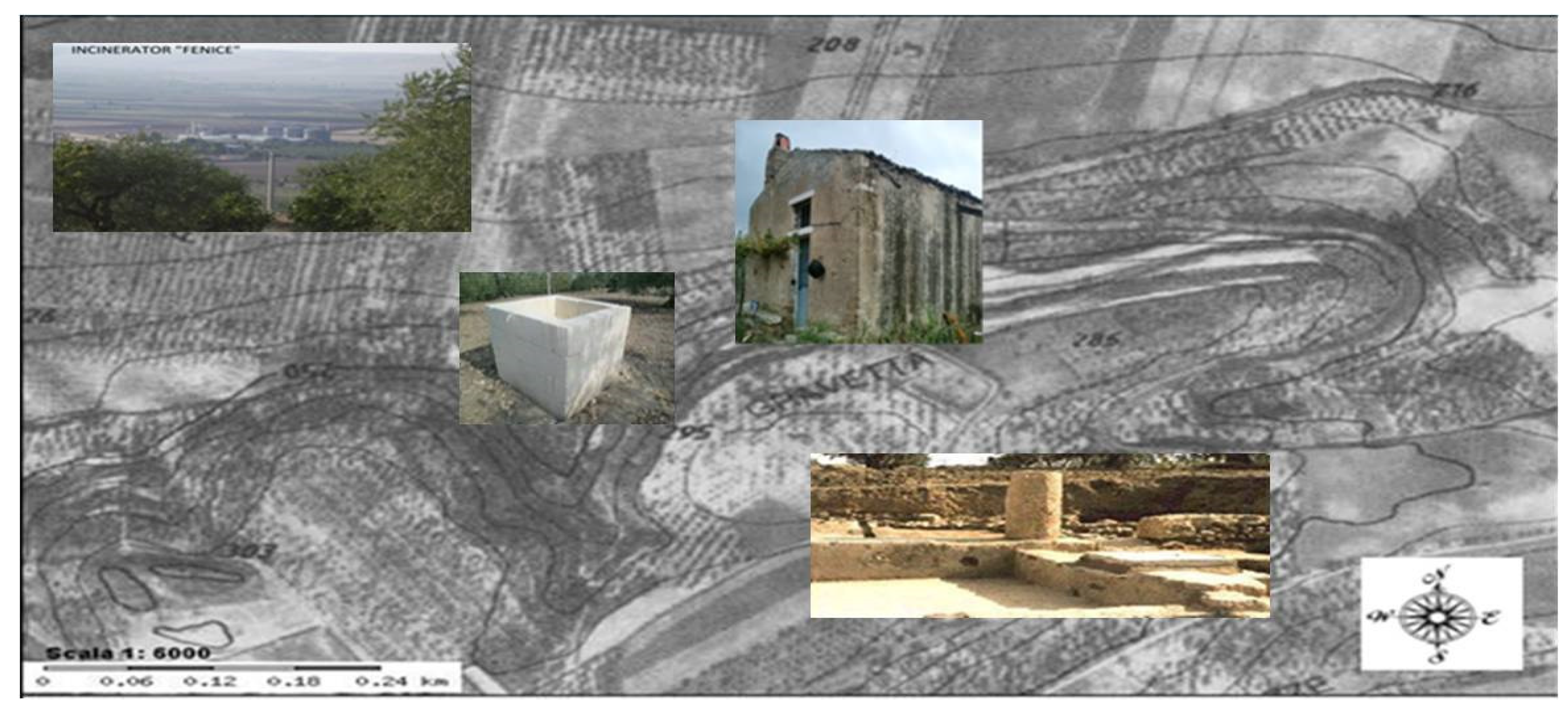
The two buildings in calcarenite studied in this work are made of stones, sourced from the same local quarry as required by the research project [
13,
14], closely located in the rural site of Basilicata, shown in
Figure 1, not far geographically from Matera.
The procedures for the collection, storage and preparation of samples for XPS analysis were based on the guidelines of the ISO committee 20579-1:2024 available online:
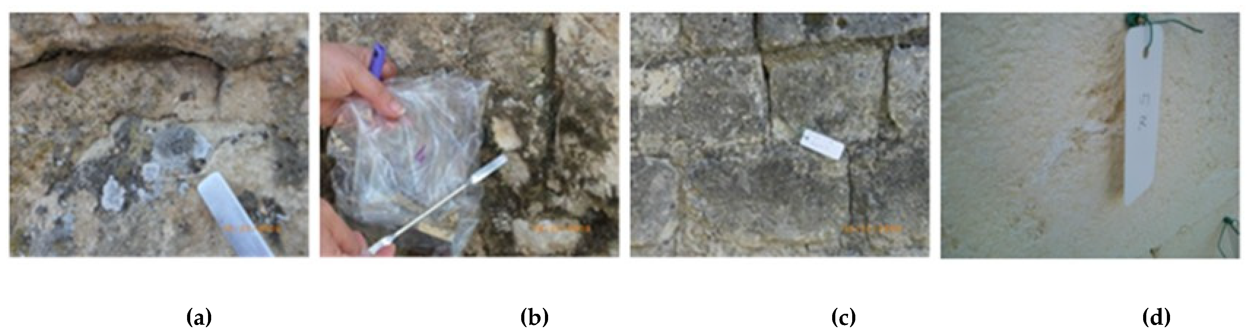
https://www.iso.org/standards.html (consulted from the publication date 2024-09, accessed on 3 July 2025). Adequate quantities of powdered samples were gently scraped from the wall surfaces of the cubic building (occasionally added to small fragments eventually detachable after years if suitable in size for the insertion into XPS sample holders), mainly from the upper half zones of each wall to avoid traces of soil contaminants, at regular time intervals of outdoor exposure at 0 (unexposed reference sample, 0R), 3, 6, 9, 12, 21 and 52 months. The 52-month period seemed appropriate for long-term sampling, given the slowing of surface changes already observed as the second year approached, and indeed, the five-year span proved to capture both the rapid initial phase and the subsequent stabilization.
Similar sampling procedures that include samples collection, storage and cataloguing, as reported in
Figure 2, were performed on the entirely preserved NE walls of the old farmhouse, selecting different colored zones:
- 1v.
Calcarenite-like surface (Blank color renewed by wind and rain erosions)
- 2v.
Efflorescent-like surface (whitish)
- 3v.
Green mossy surface
- 4v.
Black crusty surface
Figure 2.
The sampling modalities: (a) collection and (b) storage of samples; cataloguing: (c) on the north east walls of the old farmhouse and (d) on the North wall of the new cube in calcarenite.
Figure 2.
The sampling modalities: (a) collection and (b) storage of samples; cataloguing: (c) on the north east walls of the old farmhouse and (d) on the North wall of the new cube in calcarenite.
X-ray Photoelectron Spectroscopy (XPS) ensures to determine the outer layer composition of solid surfaces, i.e., within a vertical depth of 10 nm using the conventional X-rays sources of ~1500eV energy, here reported. Importantly, it provides joint information on the elements present and their chemical state by measuring the binding energy (BE) of the emitted photoelectrons and, by resolving the peak components via curve-fitting, the semi-quantitative analysis of the identified surface compounds.In summary, XPS provides detailed chemical information of the analyzed samples and interfering contaminants due to its surface sensitivity. It requires ultra-high vacuum (UHV) conditions and has limitations in depth profiling and spatial resolution.
The bulkier spectroscopy XRD (X-ray Diffraction) provides structural information of solid materials from depths of several microns, depending on the X-ray source. The diffractometer characteristics are reportedin previous work [
13], and the results obtained on the powdered samples are here recalled for comparison, taking into account thatonlycrystalline (inorganic) compounds can be revealed by X-ray scattering. A quite large amount of materials is required to produce the diffraction pattern, and mixtures of crystalline and amorphousphases can be difficult to interpret.
Scanning Electron Microscopy equipped with Energy-Dispersive Spectrometry for microanalysis (SEM/EDS) allows the morphological images (at various magnifications) of samples (in powders or thin sections) and to measure the X-ray emitted by elements from depths of a few microns for their identification and relative intensity. The SEM and EDS instruments are reported in a previous work [
14] and the unpublished PhD results, partly recalled in the
Supplementary Materials, are usefully compared with the surface composition of the same samples revealed by XPS to derive the elemental in-depth distribution likely induced by the calcarenite colonizers identified with biological essays. The joint use of SEM/EDS allows to image microbial and solid phases and the elemental relative intensity in the analyzed area with high spatial resolution but limited chemical states information.
Detailed characteristics of spectroscopy and microscopy techniques of use in the BB.CC. field are exhaustively listed in ref. [
18].
2.1. XPS Analysis
The XPS spectra of the samples collected in the five-year period were acquired with two available spectrometers, Leybold LHX1 (Leybold GmbH merged into SPECS) for most part of the research project and subsequently with the new Phoibos100 MCD5 (SPECS, Surface Nano Analysis GmbH, Berlin, Germany). Both spectrometers, equipped with double-anode, achromatic Al/Mg Kα
1,2 sources (1486.6/1253.6 eV) and KE
−1 as the transmission function, were used with the same operating modes and in parallel for repeated analyses, after having verified the close similarity of their performances with the acquisition of standard compounds. The wide and detailed spectra were all acquired at normal emission in FAT (Fixed Analyzer Transmission) and medium area (diameter = 2 mm) modes with channel widths of 1.0 eV and 0.1 eV, respectively, and the acquisition time of 0.5 s for each channel. The energy scale was calibrated using gold, copper and silver foils as the reference set for binding energies with the Au4f7/2 signal at 84.0 eV, Cu2p3/2 at 932.7 eV and Ag3d5/2 of silver at 368.3 eV [
19,
20].
Powdered samples were prepared for XPS acquisition by pressing them with a stainless steel spatula on double-sided copper tape previously fixed on a steel sample holder. The preparation was carefully performed to ensure a uniform thin layer just thick enough to avoid any signal from the adhesive tape and to prevent loose particles from contaminating the vacuum chambers by shaking and tilting the sample holder downwards, as recommended by ISO guidelines. After this operation, when the pressure in the pre-chamber was reduced to about 10−5 Pa, the sample was introduced into the analysis chamber of the spectrometer(s), where a pressure of ≤10−7 Pa had been reached, as required for ultra-high vacuum (UHV) analysis.
The acquired spectra were resolved into the component peaks and associated background using the homemade program NewGoogly, which allows the simultaneous curve-fitting of the intrinsic and extrinsic features of XPS spectra [
7,
21].
In this, as in a previous work, the figures show the spectra ‘as acquired’, while the tables with the curve-fitting results (of detailed regions) report the peak areas ‘normalized’ for the sensitivity factors (FS) associated with the orbitals of the elements under examination and the binding energies (BEs) ‘corrected’ for the surface electrostatic charging of the sample under analysis, referring to the aliphatic carbon, identified in all curve-fitted C1s spectra as the internal standard (IS) and setting its BE to 285.0eV. The BE values have an instrumental uncertainty of ±0.1 eV, but the total uncertainty, where reported (vide infra), derives from the results of repeated analysis and curve-fitting procedures.
All the identified peaks were assigned to the various chemical speciesby comparison with the standard spectra acquired in the laboratory and with those reported in the XPS database available online (
https://srdata.nist.gov/xps periodically consulted, last accessed 20 February 2025).
2.2. Principal Component Analysis (PCA)
Principal Component Analysis (PCA) was used for XPS data exploration and visualization. Among chemometric methods, unsupervised PCA is commonly considered the favorite statistical approach for deriving information from multivariate data of various types [
17]. Based on the construction of new independent variables called principal components (PCs) as linear combinations of the original variables, PCA allows to reduce the dimensionality of large datasets while retaining the maximum information, thus simplifying their interpretation [
22,
23]. The graphic outputs obtained from the Principal Component Analysis are represented by the score and loading plots: the score plot distributes the samples in the space defined by PCs highlighting any groupings and clustering among them, while the loading plot provides information about the original variables responsible for any clustering in the samples. Their joint visualization usefully improves data interpretation. Here, the R-based software CAT (Chemometric Agile Tool), available online [
24], was used to explore, with PCA, the large XPS dataset and possibly derive further information.
3. Results and Discussion
In this ‘core’ section, we will try to best show the trend of degradation for the calcarenite rocks under study by summarizing the numerous XPS data collected over the five-year period, elaborated via our well-established curve-fitting procedure [
21], and comment on their exploration and visualization with PCA using CAT software [
24].
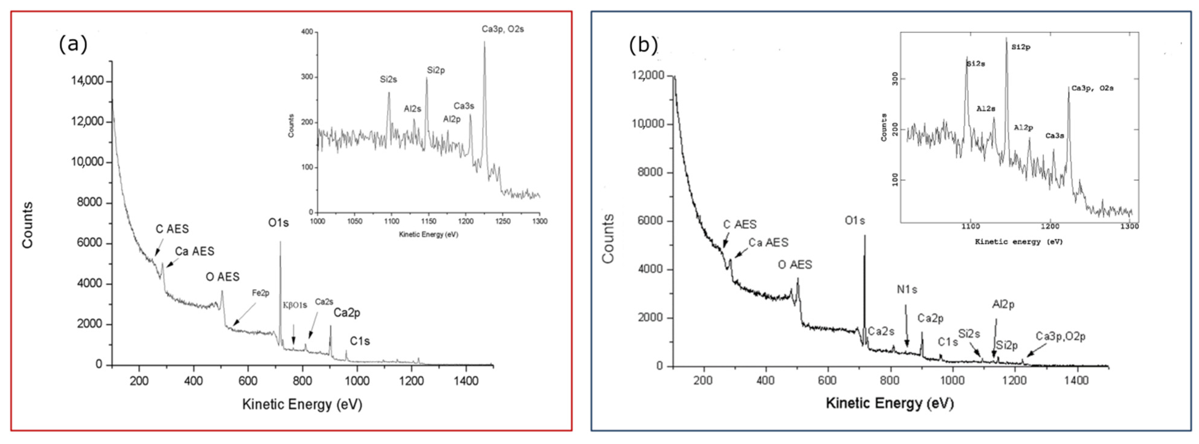
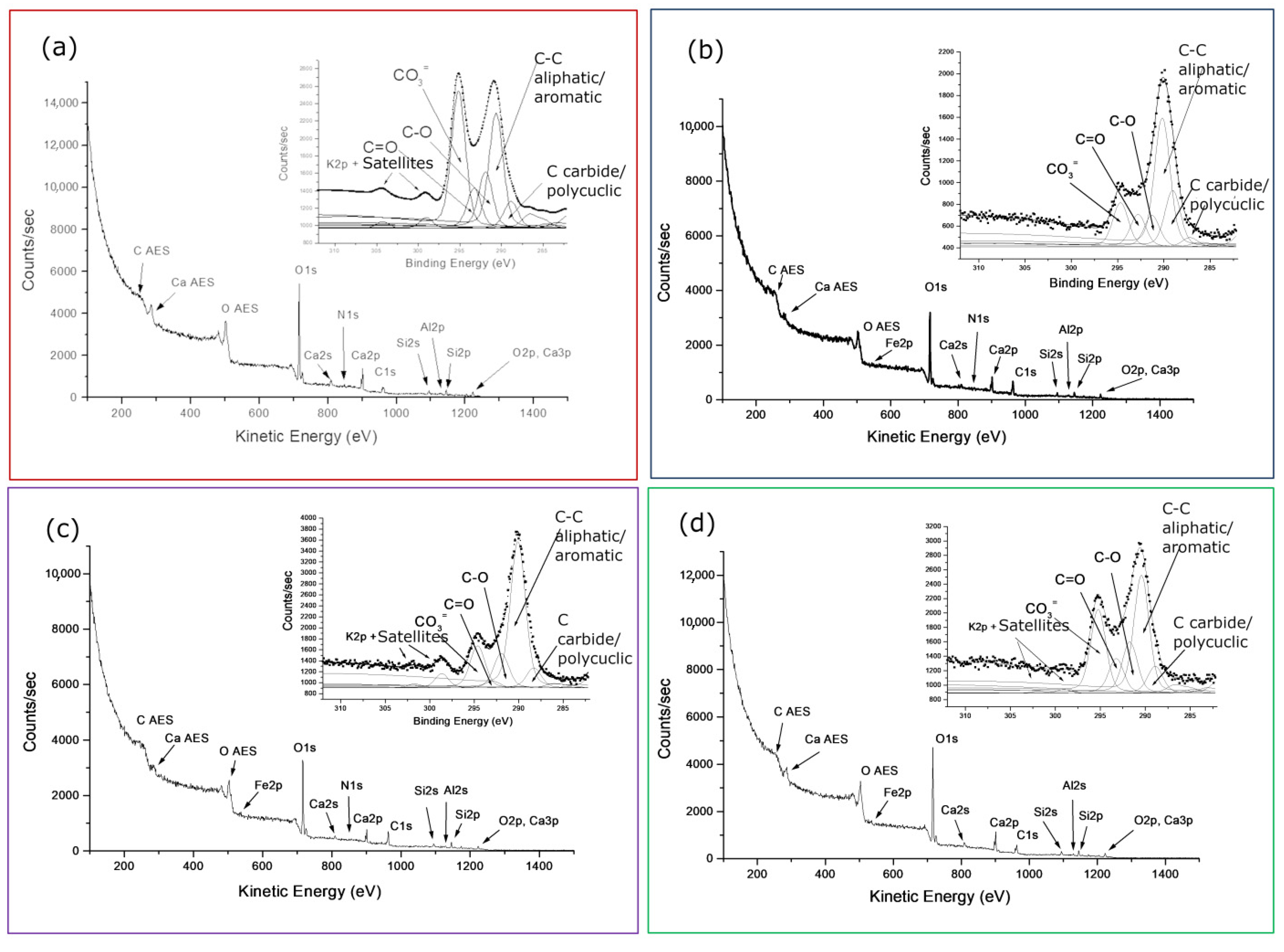
First of all, it is interesting to note, aided by the peak labeling in both wide spectra of
Figure 3, the same main elements composing the two samples with iron in traces in the ‘true’
Figure 3a replaced by nitrogen in
Figure 3b of the old farm. The ubiquity of organic particulate/functionalized carbons on calcarenitic surfaces, revealed by XPS at a nanometric depth, will also be confirmed. Such organic matter, gradually contributing to the surface layers, increasingly affects the relative intensity of the main carbonate and oxides/silicate components of the rock, as can also be seen in the insets of both spectra.
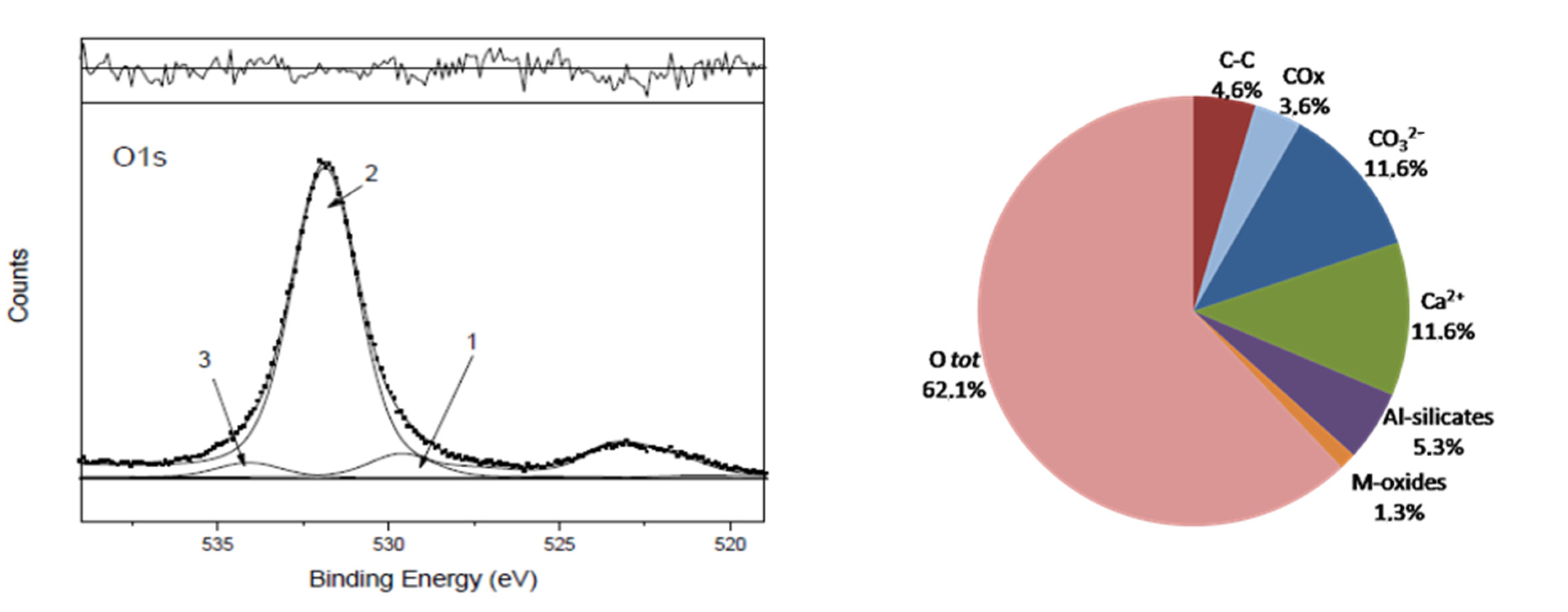
Effectively, the peak labeling in the wide spectrum of
Figure 3a better reflects the elemental composition of the calcarenite stones [
7,
15] being used to build the new calcarenite block ‘just installed’ with ‘relatively clean’ surfaces. The main regions, best representative of each detected element and its chemical states, first acquired at higher resolution and then resolved into the component peaks using ‘NewGoogly’ [
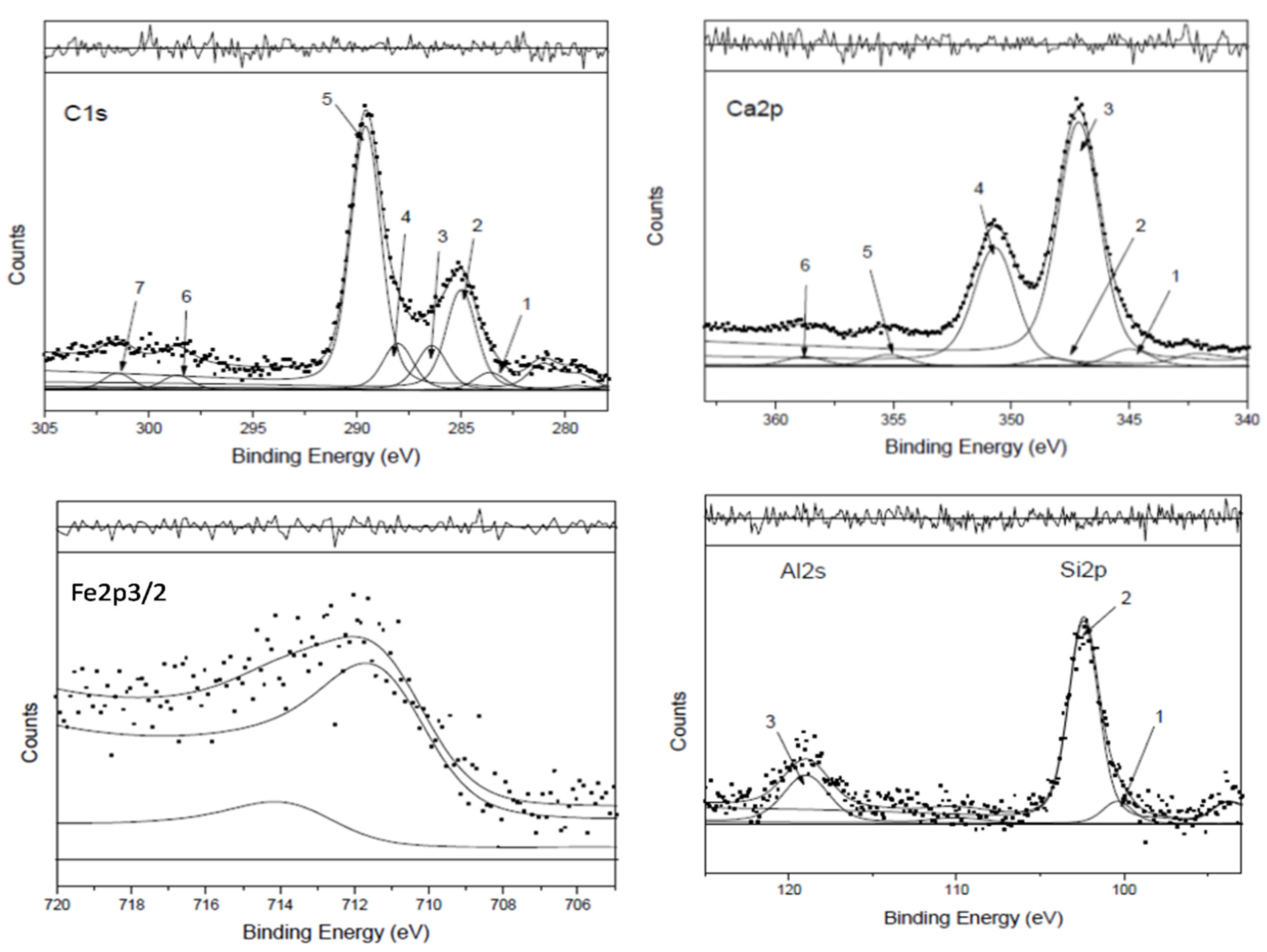
21], are reported in
Figure 4, and the correspondent curve-fitting results are listed in
Table 1 for deriving the percentage of chemical groups all detailed in the legend and shown in the pie chart at the bottom right of
Figure 4.
The peak assignments reported in
Table 1 were qualitatively validated by combining binding energy (BE) indications retrievable from the XPS database, literature and laboratory curve-fitting results of standard compounds and quantitatively by the cross-check of normalized peak areas used to perform partial and total mass balances, considered satisfactory if in the limits of XPS accuracy of +/−10% [
19,
20]. The group percentages summarized in the pie chart of
Figure 4 satisfy these premises and indicate the right area ratios for the carbonate components (carbon:calcium:oxygen ≈ 1:1:3), as for reference CaCO
3,while the sum of oxygenated contributions associated with CaO+Fe
2O
3 and Al
2O
3+SiO
2, respectively, representing M-oxides and Al-silicates using the stoichiometric coefficients of each single compound, required the addition of almost 20% of hydration water/hydroxyls, not specifically assigned, to match the total O1s area within the above-mentioned uncertainty in the area ratio.
Ca2+ and CO3= of the Carbonate structure, both reported to visualize their ratio (1:1 in reference CaCO3) (Ca2p peaks 2+4+5 and C1s peaks 5+6+7).
C-C carbide/graphitic and polycyclic carbons (C1s peak 1) + Aliphatic/aromatic (C1s peak 2): IS.
COx oxygen functionalized carbons (C1s peaks 3+4) to which CN groups can be added if nitrogen is present in aminic and/or amidic forms.
Mixed oxides*; in this case, CaO (Ca2p peaks 1+3) and Fe2O3 (Fe2p3/2 peak).
Al-silicates: Al2O3 (Al2s peak) + SiO2 (Si2p peak 2).
The oxygen percentage, arbitrarily resolved in three components (see related text hereafter) is reported in the pie chart as the O1s total area.
*Mixed oxides in reference calcarenitic rocks normally comprise Ca/Mg/K/Fe oxides not always contemporarily revealed in the surface layers. Other elements if present are reported as ‘extra’ in the captions.
As already found in a previous work [
7], it is often difficult when dealing with real samples to resolve the O1s region into the component peaks if many oxygenated groups contribute to it and their chemical states are too close in terms of binding energy, BE, for the given instrumental resolution, using achromatic X-ray sources. In this case, the three curve-fitted oxygen peaks, although belonging to differentiated classes of oxygenated compounds, characterizing the reference calcarenite 0R [
7,
15], actually are not of the right intensity to individually correspond to the oxygenated compounds defined in the assignments and identified in the corresponding detailed regions, listed in
Table 1. Therefore, also in this work, the only way to successfully perform the oxygen ‘mass balance’ is to refer all the oxygenated compounds to the total O1s area, taking into account their stoichiometry.
The curve-fitting procedure adopted for the reference sample (0R) was repeated for all the acquired XPS spectra, following the sampling interval of 3, 6, 9, 12, 21 and 52 months from the north, east, south and west walls of the externally exposed calcarenite cube, as shown in the
Section 2.
As found by the XPS characterization of sample 0R, the composition of calcarenite surfaces was already of a certain complexity in the starting/unexposed reference and, from the visual comparison of the two wide spectra in
Figure 3, it is expected to evolve over time. Indeed, the coexistence of single stoichiometric compounds identified by curve-fitting the detailed regions of
Figure 4 is certainly a simplification of the interconnected chemical bonds representing the composition of ‘real’ surfaces. However, the grouping classification, mainly consisting of mixed compounds, listed in the legend of
Table 1 and reported in the pie chart, proves very useful to verify the counterions balance so as to estimate the neutrality of the surface composition. In this way, a good assessment of their compositional variation over time can also be performed, which is necessary to extrapolate the trend of calcarenite degradation from comparative XPS characterizations.
The first processing of the XPS temporal monitoring is shown in
Supplementary Figure S1a–d, represented by equidistant analyses, three months-spaced sampling, of the cube walls, cardinally oriented, in the first nine months of outside exposure.
The XPS results related to that period were previously commented together with other instrumental techniques [
13,
14] also taking into account online data provided by the control unit of the regional agency ARPAB on the local weather and emissions from the nearby incinerator ‘Fenice’ on the wind direction and strength (retrievable by the wind rose graphic) and combined microscopy and biological analysis. In these
supplementary figures, the XPS results were re-proposed using the grouped components, equally shown in the pie chart of
Figure 4 for the reference 0R samples, as the appropriate ‘indicators’ of the calcarenite decay versus time.
As evident in
Figure S1a–d, the new building in the nine months of exposure to the outside since its installation (July 2009) showed compositional variation of its wall surfaces, the changes of the main chemical groups in their relative intensity certainly linked to the seasonal characteristics of the year (temperature, rainfall, wind, etc.):
- -
In the first 3 months, traces of other elements are seen deposited on the west, south and east walls, consisting of sulfur, phosphorus and chlorine anions, all mass balanced by sodium counter cation, most likely coming from the incinerator fumes and transported by the winds blowing from the north.
- -
After 3 months, it can be noted that the contribution of carbons, C-C and COx/CN, other than carbonates, has, ‘on average’, increased compared to the reference. This can be attributed both to the deposition of carbonaceous particles possibly contributed by the combustion process of the ‘Fenice’ incinerator (PTS) and/or to the presence of microorganism colonies, already localized and developed in the subsurface/inner areas, as attested by slight chromatic changes of surfaces and colored stains along some parts, porous and with interstices, of the cube walls and corroborated by SEM images (see the next sections).
- -
The excess of carbon carbonate compared to calcium carbonate, clearly visible in all
Figure S1a–d graphs, could be attributed to the formation of calcium bicarbonate Ca(HCO
3)
2, the unbalance attesting to the first form of degradation of calcite, the predominant component of calcarenite. In fact, when the calcarenite comes into contact with humidity and acid rainwater, the calcite hydrates and dissolves, forming carbonate complexes such as bicarbonate ions [
25,
26]. Depending on the outdoor conditions, the main carbonate structure of calcarenite can be differently hydrated, thus leading to different H
2CO
3--/CO
3-- mixtures differently balanced by calcium, while ‘mixed oxides’ may include flowing ions sharing the hydroxyls of the phyllosilicate structure and the oxygens of functionalized carbons and other combinations to be similarly verified in the presence of oxalic acid and other metabolites due to biological activities [
6,
7,
27,
28].
- -
Hydration and de-hydration processes could be followed by the oscillation percentage of oxygen for each wall during nine months. The oscillations could be the result of meteorological conditions favoring/disfavoring the synergistic actions of abiotic and biotic pollutants locally interacting with calcarenite surfaces. The calcarenite cube, from the moment of its installation, has certainly experienced hot but also rainy periods, as reported by the portal of the Lavello weather station (
https://www.3bmeteo.com/meteo/lavello/storico (accessed on 3 July 2025), periodically accessed during experiments). The high temperature and the abundant rainfall represent the fundamental conditions for condensation phenomena to occur, which constitute an extremely efficient transport mechanism for atmospheric pollutants. In fact, while the rain immediately removes the products resulting from the attack of the original material, the condensation water, not normally being sufficient to flow on the surface, evaporates, leaving behind reaction products that can give rise to further destructive processes, eventually with disintegration of the surface area itself [
8,
29].
Obviously, XPS observations of the cubic calcarenite after only 9 months of outdoor exposition do not allow to identify clearly the prevalent factors and/or their combined actions responsible for its decay. It was already possible, however, to notice that, while the first quarterly sampling showed some variation in the composition of the cube walls due to the wind blowing from the north, carrying additional elements (extra in the legends) mainly in EWS directions, later on, the XPS differentiation was no longer so evident, and gradually, the effects of the environmental interactions on the four walls could be considered averagely comparable.
It was therefore decided to graphically represent the degradation trend of cubic calcarenite, expressed by the percentage intensity versus time of the component groups, averaged over the four walls, with the associated standard deviation. In the
supplementary ‘average’ plots, Figure S2, two options are presented: in
Figure S2a, the percentage of oxygen is retained to also control the variation of the average degree of hydration (i.e., the hydration de-hydration oscillations observed for the single walls), while, in
Figure S2b, the oxygen is omitted to enlarge the scale and therefore better estimate the behavior of the component groups, the total area of the O1s region being implicitly considered as the stoichiometric sum of all the oxygenated compounds. The comparison of the two
Figure S2 plots shows that the trend in the nine-month interval is indeed mainly characterized by the variations of the component groups, to be thus confirmed as the main indicators of degradation; therefore, the
Figure S2b option was chosen to complete the plot of calcarenite decay over time to also simplify the processing and visualization of the larger dataset without considering the total oxygen percentage as an additional variable.
The subsequent and final phases of the project specifically concerning the temporal monitoring of calcarenite by XPS were then considered in the following order:
As already specified in the
Section 2, the samples were taken on the north east walls of the old building following the sampling sequences reported in
Figure 2 and selecting the four specific zones, different in their appearance, therein indicated.
The wide spectra of the four colored samples with associated peaks labeling and the curve-fitted C1s regions inserted are compared in
Figure 5. The overall percentage composition derived by curve-fitting, without the total oxygen percentage, is reported in
Table 2 using the same grouped components retrieved for the reference 0R sample, with no extra elements detected by XPS.
Table 2 shows the curve-fitting results of the old building samples 1v–4v, in percentage form according to the
Figure S2b option, and those correspondent to sample 0R of the new building added for comparison. We can now better judge the differences of the two references, 0R and a-1v, for the new and old buildings, respectively, qualitatively predicted by comparing their wide spectra in
Figure 3. We can also extend the comparison to the remaining samples 2v–4v, all together representative of the old farm building, and derive some anticipations on the evolution of the surface compositions due to their very different aging times.
Observing the four spectra in
Figure 5a–d with the related grouped components listed in
Table 2, the surface increase of the carbonaceous components, including nitrogen- functionalized carbons, and the inverse intensity of the carbonate and silicate components, compared to the reference sample of the new building, seem to be the prevalent indications of long-weathered calcarenite, common to samples 1v–4v of the old building,
independently of their very different appearances.
Indeed, the strong inversion of the silicate/carbonate ratio and the consistent organic deposits on the walls of the old farmhouse respond well, respectively, to the expected prevalent dissolution of the carbonate compared to the silicate constituent [
8,
9], which is a minority in the calcarenite rock, and to the ubiquitous presence of superficial patinas/biofilms [
10,
11,
12] stabilized over time.
Taking into account the above considerations, the reason for the colorations that visually differentiate the samples in
Figure 5 could then be traced back to biological processes occurring at greater depths than the outer surfaces, probably originally colonized, therefore visible to direct observation and detectable by the complementary techniques in use during the research project [
13,
14].
All these aspects that emerged from the monitoring of the old farmhouse in direct comparison with the 0R sample (from unexposed cubic calcarenite) will be reconsidered with the completion of the temporal monitoring of the new building, illustrated in the next paragraph. The final phase was dedicated to the processing of the entire dataset obtained in the hope of deriving useful information on the degradation processes of calcarenitic stones: their onset and their temporal evolution and, finally, their possible stabilization/convergence over time.
The data matrix in
Table 3, in the percentage format of
Table 2, represents the entire collection of XPS results, obtained through periodic monitoring of the four walls of the new cubic construction. It begins with the unexposed 0R and adding the four walls results up to 52 months of outdoor exposition and, according to the project objective, the results of the four samples (1v–4v) from the old farmhouse for the ultimate comparison. Moreover, for each sample/sampling time, the binding energies (BEs) of the Ca
2+ and CO
3-- carbonate components, the main structural constituent of calcarenite, are included as additional variables for PCA to verify their variation in relation to weathering modifications of the carbonate structure.
XPS Data Matrix
At% composition resulting from the curve-fitted spectra of the four walls of the cubic building at the reported sampling time, with the exception of the sampling after six months performed only on two walls, N/E, and the four NE samplings of the old building (1v–4v).
The last two columns with the (corrected) BEs for Ca2+ and CO3= peaks of the carbonates at each sampling were included as additional variables for PCA to verify the BE chemical shifts versus reference calcarenite 0R as a function of time.
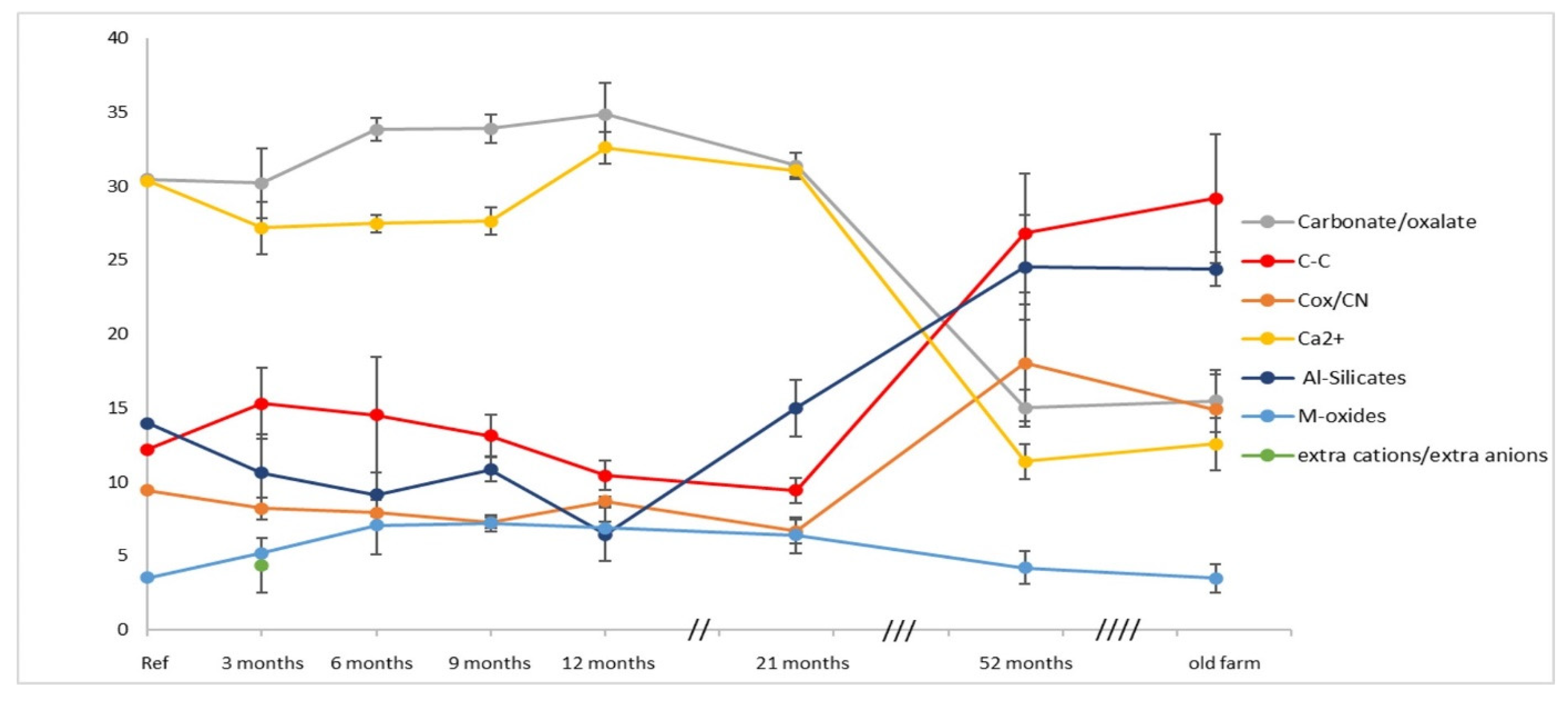
Figure 6 shows the completed S2b plot using, of all the curve-fitted data reported in
Table 3, the average of the same chemical groups (XPS indicators of degradation, listed in the legend) present on the four walls of the new building at each sampling time and, similarly, the average of the four samples collected from the walls of the old building (old farm). As anticipated, the decay trend based on the
Figure S2b option seems more justified with the increasing time, in particular, for the new building, given its small size. Therefore, the contributions averaged on all oriented faces are more appropriate, and the balance of their hydration/dehydration percentage observed in the nine-months interval better justifies the omission of the total oxygen area as a ‘decay indicator’ being implicitly accounted for by the total contribution of oxygenated compounds, verifiable a priori during the curve-fitting procedure.
The sampling variability across the four walls, shown by the ‘error bar’ of each decay indicator in
Figure 6, is represented by the standard deviation associated with the mean value of the four collected samples. Instead, as said and shown in
Figure S1 for single samplings, the uncertainty associated with the reference sample 0R is to be considered equal to +/−10% [
19,
20] and therefore doubled in the case of only two samples collected at 6 months.
The compositional changes already observed after three months are progressing, maintaining the trend over the course of the first year of exposure, with the variability ranges reflected in the magnitude of the standard deviations associated with the means. The percentage variations are clearly linked to the different contribution of the individual walls, evident in
Figure S1a–d classified by cardinal orientation. In
Figure 6, the influence of meteorological fluctuations and washing away of the wall surfaces by precipitation with the consequent removal of the crystallized salts present on the surfaces (‘extra cations/anions’ in the graphs) and other reasonable differences in the composition of the sampling zones are all included in the variability associated with the ‘averaged’ indicators of samples collected from different walls/areas of the cubic building.
After the first year, sampling was no longer scheduled every three months; however, at the end of the year, after the 12 months of sampling, the imbalance of the carbonate components tended to be reduced, then reached with the sampling at 21 months. Subsequently, the percentage inversion of carbonates and Al-silicates was already predictable in the graphic trend, fully achieved after 52 months of sampling, clearly represented by a progressive decrease in calcium and carbonate carbon and by a strong increase in silicates and aliphatic/aromatic and functionalized carbons.
Interestingly, in the absence of intermediate sampling, it can be inferred that the exposure time prolonged over two years leads, at some stage, to a sort of stabilization of the degraded calcarenite, at least regarding the similarity of the surface composition for both buildings, as evident in the last part of the graph in
Figure 6. Indeed, the ‘same’ component groups, of nearly the ‘same’ percentage distribution, within the indicated error bar characterize the averaged samples collected from the new building (52months of sampling) and old (1v–4v sampling) farmhouse.
The trend shown in
Figure 6 highlights the decay phenomena that can be justified by the continuous dissociation and dissolution of the carbonate matrix and by the concomitant increase in aliphatic/aromatic carbons due to the deposition of incombustible carbon particles and of functionalized carbons probably accentuated by the presence of lichens and algae, as shown in the SEM (Scanning Electron Microscopy) images acquired on the samples collected after 12 months of exposure from the cube walls [
13,
14]. Some images with included EDS microanalysis are reproduced in
Supplementary Figure S3, together with the list of identified bacteria of the genus
Bacillus, available from the (unpublished) PhD thesis. The presence of lichens in the subsurface zones supports the hypothesis according to which the calcarenite rocks, in addition to the evident degradation of their carbonate matrix due to atmospheric agents and acidity of rainwater, undergo an increase in porosity augmented by freeze–thaw cycles [
8,
9,
29]. As experimentally verified with timed tests on the capillarity of calcarenite stones ([
13,
14] and PhD report), the expansion caused by the internal pressure exerted by frozen water promotes biocolonization. The colonizing microorganisms that tend to settle inside the pores and interstices of the stone material induce the reduction of the interstitial porosity, as shown in
Figure S3.
The evolving stages of colonization were testified by the biological analysis anticipated in the Introduction, carried out on samples taken from the walls of the cubic building at the end of two years of exposure and, for comparison, also from the walls of the farmhouse. The same microorganisms were found, using the analytical techniques mentioned above for both buildings, and similarly distributed on the surfaces (bacteria belonging to the Bacillus family, listed in
Figure S3) and beneath surfaces (lichens/fungi listed in ref. [
14]) on inner faces more protected from environmental threats together with mono- and di-hydrated calcium oxalates detected by XRD (PhD report), derived from the dissolution of carbonates by oxalic acid, one of the bio-metabolic products.
The degradation trend of calcarenite outlined in
Figure 6 fully accounts for the bioactivities of the ‘same’ colonizers in determining the surface composition of the new building walls to evolve towards that of the old building walls, left exposed to the outside in similar conditions for over a century. In fact, the averaged results from the XPS analyses of the four samples considered in
Figure 5 and
Table 2, so different in appearance, as widely specified, align perfectly with those of the new building at the last sampling (after 52 months), within the limit of the total variability due to sampling, to the calculation of the curve-fitting, as well as to the orientation of the walls and to the characteristics of the samples themselves, the latter expected with greater specificity given the dimensions of the old building and, therefore, of sampling areas with probable different exposure even along the same wall.
Principal Component Analysis (PCA) was finally applied to the entire XPS dataset of
Table 3, using the R-based version 3.1.2 of the CAT software available online [
24], with the aim of evaluating the information content of the variables while reducing their number, eliminating the redundant ones. The matrix includes 22 surface samples of calcarenite collected at the given time intervals, the blank calcarenite 0R, 4 samples of the old building (1v–4v) and 8 variables, i.e., the percentage of the chemical groups listed aside the XPS graphs of
Figure 6 plus Ca
2+/CO
3= binding energies (BEs) known to be sensitive to the calcium carbonate structural changes [
25,
26]. The graphical output of the CAT software is shown in
Figure 7a–c where the combined display of the three graphs, scree, scores and loading plots helps the interpretation of the data to rationalize the degradation processes under consideration.
A scree plot illustrating the distribution of variance among the principal components is provided in
Figure 7a, offering visual evidence of component selection. A total variance higher than 80% was explained by PCA, with the two first components PC1 and PC2 able to explain the compositional variation of ‘calcarenite’ under environmental exposure and extract the main indicators of degradation.
Three main clusters were observed in the score plot, distributed along PC1 (63.3% of the explained variance). Samples collected from the new building after 52 months of exposure and from the old building,1v–4v were located on the same side of the plot, thus suggesting the same surface composition of the long-weathered samples. On the opposite side of the score plot, samples collected within 3 and 21 months were present. In detail, two main clusters were observed in this section along PC2 (18.2% of the explained variance): the first, widely distributed, included 0R and the four wall samples collected in the first nine-month time interval, the second actually consisting of two overlapping clusters each made of samples collected from the cubic walls after 12 (red cluster) and 21 (green cluster) months very closely distributed.
From the loading plot view, the variables mostly contributing to the first principal component PC1 were detected, i.e., (%Al-silicates, %C-C, %, COx/CN) and (%Ca
2+, %CO
32−/C
2O
42−, %M-oxides), which were inferred to be negatively correlated with each other. Thus, by increasing the outdoor exposure, an increased content of aliphatic/aromatic and functionalized carbons of Al and Si (grouped as Al-silicates in
Figure 6) could be noticed while decreasing the content of carbonates and mixed-oxides.
The PCA plots of
Figure 7 overall agree with the XPS plot of
Figure 6 and support the interpretation given on the decay trend of calcarenite over time. Moreover, another agreement concerns the BE behavior of Ca
2+ and CO
3=, the carbonate constituents, considered as additional variables for PCA, mostly contributing to the PC2 component. Viewing the score and loading plots together, it can be seen that their BEs increase with outdoor exposure in the first year. In fact, even considering the variability range that goes beyond the energy step (+/−0.1eV) only reported in
Table 3, the BEs listed therein record the concomitant increase for the two constituents, up to their maximum values, 348.0 eV(Ca
2+) and 290.2 eV(CO
3=), right in the time interval of the two clusters and the subsequent decrease, although not always to the same extent, for the samples collected from the cubic walls aged 52 months and the old farmhouse.
The variations in the binding energies of the carbonate constituents and in their ratio are clearly conditioned by the temporal impact of the abiotic and biotic agents on the calcarenitic walls, monitored in this work by their XPS characterization; therefore, they could be regarded as an integrative part of the set of degradation trend indicators reported in
Figure 6, as hereafter summarized.
To start with, the weathering susceptibility of carbonates to dissolve and form Ca(HCO3)2 is mainly responsible for the recurrent Ca2+ < CO3= ratio, most visible in our graphical percentages up to nine months of outdoor exposure. In subitaneous succession, the reported attachment of autotroph microorganisms takes place and the calcarenite colonization proceeds with the cooperation of different heterotroph lithotypes mutually interacting for the construction of a protective biofilm, as indirectly testified by the increase in carbonaceous components in the surface layers and directly by SEM, XRD and biological analysis, already mentioned.
Among the metabolic routes of the bio-colonizing communities are those responsible for dissolution by Ca
2+ complexation and those of reprecipitation, the reprecipitate CaCO
3 clearly structurally different from the pristine calcite and thus presumably of different BEs [
10,
11,
12,
27,
28]. From the graphical trend of
Figure 6 and data matrix of
Table 3, the time required for the adhering biofilm to consolidate onto calcarenite and then structurally evolve for the living of cohabitant microorganisms apparently ranges around two years or less, judging from the BE values of the samples collected at twelve and twenty-one months, further supported by the better equivalence of Ca
2+:CO
3= percentage of the last, likely due to the reprecipitation of calcium carbonate, contributing in the outermost layers.
Considering all the points paid attention to so far, the main features that characterize long-exposure calcarenitic surfaces and that most capture attention in
Figure 6 are the following:
Carbonaceous C-C added to functionalized carbons (COx/CN) are the prevalent components of the surface layers, closely followed by Al-silicate groups in second place, even with the inclusion of M-oxides placed at the lowest percentage, if considered as ‘intricate’ parts of the silicate framework [
30].
Contrary to the bulk composition of calcarenite and differently from the surface composition 0R, in the highly degraded surfaces, the carbonates are the minor components, confirming the negligible degradation of the silicates, which become the major components, most probably ensuring with their solidity the surface adhesion required for the formation of a structured biofilm (with trapped pollutants) for the protection of the living microorganisms [
10,
11,
12].
The non-equivalent intensity of the carbonate constituents, visible on long-exposed surfaces, may contribute carboxylic anions, belonging to extracellular polymeric substances (EPS) produced by microorganisms and bindingCa
2+ [
27,
28]. Unfortunately, the intrinsic resolution of conventional XPS often prevents properly resolving detailed spectra into energetically close components, as reported for the curve-fitted O1s region. Even in the case of the curve-fitted Ca2p and C1s regions, for the peaks generally assigned to ‘calcium carbonate’ constituents, the co-presence of unresolved components can be reflected/estimated only by the Ca
2+/CO
3= ratio and the chemical shift (ΔBE) of the peaks maximum, both dependent on their relative intensity.
As a summary dissertation of this work, it can be stated that, even with all the mentioned approximations, the XPS results provided by the curve-fitting procedure [
21] (homemade NewGoogly software), confirmed by PCA using the CAT software available online [
24], seem consistently significant. The evident compositional similarity, achieved in a relatively short time, of the new weathered building with the old farmhouse clearly indicates that the degradation of the calcarenitic surfaces evolves towards a sort of stabilization, creating favorable conditions for the sequential settlement of the same microorganism community, as revealed by biological analysis.
If the right protection mechanisms (EPS, pigments and internal shelters) are then activated for the survival of the biocolonization against external attacks, all the activities of the cohabiting microorganisms necessary for their life and for the consolidation of the surface layers, in the form of a protective structured biofilm, reach a dynamic equilibrium that can persist for an indefinite time.
The importance of biofilms that develop on external monuments and their dual role [
31], protective on external surfaces and erosive when they protrude internally, is still a matter of debate, as it was a decade ago, when the experiments reported in this work were conducted. Attempts have been made to identify antagonistic bacterial/fungal microorganisms and to extract their metabolic products (toxins) to be used for the removal of biofilms by natural cleaning (bioremediation) in the place of traditional chemical products ([
7,
27] and SCN publications cited therein).
Bioremediation has proven effective in some cases but not in others when the removal of the biofilm induced a greater reactivity of the renovated surfaces with impediments to consolidation actions and therefore a timely regression to the structural degradation of the monumental walls. Numerous case studies have shown the importance of appropriate diagnostics to evaluate case by case the relative importance between the protection and the destruction of calcarenitic stones by microorganisms in order to plan the most appropriate interventions.
We believe the results reported here represent a useful piece of information supporting the research nowadays, recently reviewed for the use of multi-techniques and multidisciplinary approaches with the support of new technological advancements [
31] under the UNI 111882:2006 Standard Protocol [
32] and ICOMOS’s guideline recommendations (available online:
https://www.icomos.org, accessed on 3 July 2025).
4. Conclusions
This work reports the five-year XPS monitoring of two calcarenite buildings, a newly installed cubic block and an adjacent old farmhouse, exposed to the outside, with the aim of clarifying the chemical indicators and the degradation pathways of calcarenite from the initial to the advanced stages.
The interpretation of the large dataset obtained with XPS temporal monitoring was aided by the comparison of the complementary results provided in the first two years of the project using combined techniques, some reported in
Supplementary Figure S3, and by referring to the most recent acquisitions of the literature dedicated to the monumental heritage cited in this work. Another important remark regards the support of chemometric methods—in this case, the unsupervised PCA exploration of the large XPS dataset. The trend of calcarenite degradation fully reported in
Figure 6, starting from the reference calcarenite and projected through the sampling sequence up to 52months, towards the surface state of the ancient farmhouse finds exactly the same temporal correspondence in both PCA graphs, score and loading plot, displayed together and jointly interpretable in
Figure 7.
The decay indicators identified by XPS, using the well-established curve-fitting procedure, can therefore validly represent the surface composition of the external calcarenite monuments and their variations over time under the given conditions. In particular, in our rural site, having limited the sampling to the upper areas of the two buildings not affected by soil interference, spontaneous vegetation growth and other large-scale invaders, the close similarities in their surface compositions may signify that the calcarenite monumental heritages, located outdoors in restricted and controlled areas, locally affected by unavoidable meteorological factors, pollutants and biological attacks, similarly deteriorate and can be monitored by surface analysis using the percentage variation of the derived indicators, referring to unexposed calcarenite, to trace the state of deterioration and plan subsequent interventions.
The surface percentage of indicators could also be indirectly indicative of concomitant processes occurring below the surface, to be directly clearly confirmed by other suitable techniques with proper analytical depths. For example, the comparison of EDS composition in deeper layers (see in
Figure S3 the combined microanalysis of the samples from the new building walls after one year of exposure and the bulk calcarenite) with the XPS composition reported in
Table 3 for the same walls at 12months,12M, even considering the different lateral resolutions of the two techniques, may provide further clues on the degradation processes. In fact, taking into account the presence of microorganisms at safer internal depths, shown by their hyphae propagation with SEM images and of the segregation of minerals revealed by EDS microanalysis, it looks like the increased content of whatever components below the surfaces correspond to their depletion on the surfaces, as, for example, encountered with ‘extra cations/anions’ no longer visible at the surface after the first months of exposure and/or mixed oxides strongly reduced over time.
In summary, despite the proximity of the industrial area to the north west with the ‘Fenice’ incinerator (perhaps not fully operational at the time, given the microscopic evidence of lichen proliferation, sensitive to high pollution) from the observation of the graphic trend of
Figure 6, two years seems to be the critical time period after which the interactive abiotic and biotic phases and the adaptation of the pioneer colonizing microorganisms converge towards the completion of well-structured biofilms and are strongly adherent to the calcarenitic surfaces and interfaces, necessary for the survival and growth of the bio-community with the arrival of new microorganisms, all cooperating against the adverse factors affecting the monumental heritage exposed outdoors.
The methodological approach and the information obtained with the temporal monitoring of the calcarenitic walls will be part of the innovative diagnostics proposed by the Tech4You PNRR (National Recovery and Resilience Plan) research projects of the University of Basilicata, specifically aimed at safeguarding and enhancing the natural and cultural heritage to mitigate the impact of climate change and strengthen local identity.


 ,
, 


