A Fault Detection Framework for Rotating Machinery with a Spectrogram and Convolutional Autoencoder

Abstract

In modern industrial systems, establishing the optimal maintenance policy for rotating machinery is essential to improve productivity and prevent catastrophic accidents. To this end, many machinery engineers have been interested in condition-based maintenance strategies, which execute the maintenance activity only when the fault symptoms are detected. For more accurate fault detection of rotating machinery, vibration signals have been widely used. However, the vibration signals collected from most real rotating machinery are noisy and nonstationary, and signals from fault states also rarely exist. To address these issues, we newly propose a fault detection framework with a spectrogram and convolutional autoencoder. Firstly, the raw vibration signals are transformed into spectrograms to represent both time- and frequency-related information. Then, a two-dimensional convolutional autoencoder is trained using only normal signals. The encoder part of the convolutional autoencoder is used as a feature extractor of the vibration signals in that it summarizes information on the input spectrogram into the smaller latent feature vector. Finally, we construct the fault detection model by applying the one-class classification algorithm to the latent feature vectors of training signals. We conducted an experimental study using vibration signals collected from a rolling element bearing experimental platform. The results confirm the superiority of the proposed fault detection framework on rotating machinery. In the experimental study, the proposed fault detection framework yielded AUROC values of almost one, and this implies that the proposed framework can be sufficiently applied to real-world fault signal detection problems.

1. Introduction

Most modern equipment systems, including motors, pumps, compressors, fans, and automobile transmissions, are comprised of rotating machinery [1]. Sudden faults (e.g., breakdown or malfunction) of that rotating machinery, including rolling bearings, often cause unnecessary interruption of processes, and this eventually degrades productivity or even results in catastrophic human accidents [2]. To counteract these problems in various industrial fields, an appropriate preventive maintenance (PM) strategy for the rotating machinery should be established. The PM strategy attempts to prevent the unexpected faults of rotating machinery by detecting machinery fault symptoms in advance of fault occurrence [3]. The PM strategy can be categorized as time-based maintenance (TBM) and condition-based maintenance (CBM) [4]. TBM is a maintenance strategy to periodically inspect or repair the equipment, whereas in CBM, the inspection or repair is performed when the symptoms of equipment faults are detected. Compared to CBM, TBM may be a more inefficient maintenance strategy because it often entails excessively frequent interruption of machinery operations for unnecessary inspection [5]. Hence, in this study, we mainly concentrate on how to more effectively execute CBM.

To execute the CBM for the rotating equipment, firstly, operating states of the equipment should be precisely diagnosed in real-time. Then, if incipient fault symptoms are detected, preventive actions (e.g., repairing the whole rotating system or replacing degraded components with new ones) are taken. Therefore, fault detection and diagnosis (FDD) techniques are a prerequisite for more successful execution of CBM for the rotating machinery.

The FDD techniques are generally divided into physics model-based and data-driven approaches. Physics model-based approaches rely on rigorously designed mathematical models to describe the dynamics of the rotating machinery. In the mathematical model, the inconsistency value between the model’s outputs and system measurements is computed, and it quantifies the level of rotating machinery faults [6]. Because of their theoretical rigorousness, the physics model-based approaches are only available when assumptions regarding the dynamics of the rotating machinery are satisfied [7]. However, as for the complex and sophisticated modern rotating machinery, it is difficult to properly formulate mathematical models to describe their dynamics, and the parameters of those mathematical models are also not accurately estimated [8]. In contrast, data-driven approaches do not require any assumption on the dynamics of real machinery systems. Furthermore, these approaches can achieve robust and reliable FDD performance when sufficient operational data are available and appropriate analytical techniques are utilized [8]. In recent years, owing to the rapid development of data acquisition and storage techniques, industrial systems have collected enormous operational data of machinery equipment in real-time. Especially, rolling bearings are fundamental components in these industrial machines, and this CBM primarily relies on monitoring vibration signals of the rolling bearings. Hence, in this study, we utilize the signal data collected from the rolling bearings [9].

Recent studies regarding FDD have utilized signal data obtained from various sensors, including vibration, acoustic, and thermometric channels. Among them, vibration signals are the most frequently used because information on operating states of the rotating machinery is directly reflected in vibration signals [10,11,12]. Nevertheless, the raw vibration signals should be simplified by summarizing them into several features because they are not easy to directly analyze. To more properly facilitate the vibration signal data, meaningful features of the signals should be extracted to identify their inherent properties. Accordingly, feature extraction is an essential procedure in signal-data-driven FDD for rotating machinery.

In most previous studies, feature extraction has been performed on the signals represented within either the time domain or frequency domain. However, in these single-domain-represented vibration signals, informative properties cannot be successfully revealed when the signals are noisy and nonstationary [13,14]. In real-world settings, the vibration signals obtained from rotating machinery are prone to being contaminated by noise due to sampling errors and uncontrollable physical interactions within the system [15,16]. Moreover, in these situations, the working environments or the operating settings of the rotating machinery often change dynamically, resulting in an inhomogeneous signal data generating process. Therefore, the time-varying patterns of frequency spectrums cannot be explicitly revealed in the single frequency domain-represented signals.

Consequently, in order to draw more useful features from the raw vibration signals, we attempt to incorporate both time- and frequency-domain information through the spectrogram. The spectrogram can be considered as two-dimensional image-formatted data, which represents the varying pattern of the frequency component’s intensity over time. To generate the spectrogram, the raw vibration signal is transformed into a two-dimensional matrix whose element indicates the intensity of a pair of certain frequency components and time points.

Then, we exploit a convolutional neural network (CNN) structure in extracting features from a spectrogram because this neural network structure is specialized to analyze the image-formatted data. The CNN structure is comprised of two types of layers, convolutional and pooling layers, and those layers are used to generate features from two-dimensional matrix inputs. The conventional CNN is basically designed for supervised learning, and hence, most previous studies on the CNN structure-based FDD have only focused on classification of the operating states or fault types. That is to say, in most previous studies, sufficient label information on the operating conditions of rotating machinery should have been prepared in advance. However, compared to normal signals, the fault signals obtained from the malfunction of machinery rarely exist in real situations [17]. Moreover, because of the scarcity of the faulty signals, properties of each individual fault type cannot be properly learned.

Thus, for the FDD without any label information on machinery faults or malfunctions, we propose to use other variant versions of CNN for unsupervised learning, which is the convolutional autoencoder (CAE). The CAE is based on the stacked autoencoder (SAE) structure that projects the input signals into small latent feature vectors. The optimal AE structures can be obtained by minimizing the errors between original inputs and reconstructed ones from those small latent feature vectors. Consequently, the latent feature vectors can summarize the intrinsic characteristics of the original input signals in order to minimize the reconstruction error. The CAE may outperform traditional SAE in handling the spectrogram by substituting fully connected layers with convolutional blocks composed of both convolutional and pooling layers. In the proposed fault detection process, the CAE model is trained only using the spectrogram collected from the normal operating state, and by doing so, the latent feature vectors in the CAE can summarize as much of the information on normal operating states as possible.

In the proposed fault detection framework, final fault detection models are constructed by using the latent feature vectors obtained from the CAE with spectrograms of normal vibration signals. However, in the current study, we postulate the problem settings that only normal vibration signals are available in the training phase. To cope with a lack of fault signals in the training phase of the fault detection model, one-class classification (OCC) algorithms can be used. The OCC algorithm builds a decision boundary using only the target class, corresponding to normal vibration signals, and the decision boundary determines whether a newly collected signal belongs to the target class or not. Up to now, numerous OCC algorithms have been proposed, and most of them are based on the data description techniques, including k-nearest neighborhood (k-NN)-based approaches, clustering analysis, and support vector-based models, and thus, more sophisticated boundaries can be obtained. In the fault detection model, the newly collected signal falling outside the boundary is rejected as an anomaly corresponding to a fault signal, whereas those located within the boundary are accepted as normal ones. Among various OCC algorithms, in this study, we considered the following: Hotelling’s T² statistics, mixture of Gaussian (MoG; [18]), Parzen window density estimation (PWDE; [19]), one-class support vector machine (OCSVM; [20]), isolation forest (IsoForest; [21]), and local outlier factor (LOF; [22]), which have shown decent performance in many fault detection problems. The main contributions of the proposed fault detection framework can be summarized as follows:

• Owing to short-time Fourier transformation (STFT)-based spectrograms, information on time-varying patterns of frequency components can be revealed. By doing so, intrinsic properties of noisy and nonstationary signals can be successfully utilized for fault detection on rotating machinery.
• Because the convolutional blocks in CAE are specialized to generate features from the image-formatted data, latent feature vectors obtained by CAE can extract more informative features from two-dimensional spectrograms.
• The OCC algorithm helps to build elaborate decision boundaries under the situations wherein counter classes (i.e., fault signals) are not available, which is frequently encountered in many real industrial fields.

The rest of this paper comprises the following: Section 2 summarizes related works on FDD for rotating machinery with vibration signals. Section 3 presents a detailed process of the proposed fault detection framework for the rotating machinery. Section 4 describes an experimental study to demonstrate the effectiveness of the proposed fault detection framework. Finally, the concluding remarks on this study are presented in Section 5.

2. Related Works

2.1. Feature Extraction for Analyzing the Signals

The vibration signals often directly reveal information on the operating state of the rotating machinery [9,10]. Hence, most of the existing works on the FDD of the rotating machinery are based on vibration signals obtained from the accelerometer sensors. To analyze the vibration signals, several informative features summarizing intrinsic properties of the raw signals should be drawn beforehand. For this reason, various feature extraction techniques for the FDD have been developed during the last decades.

Table 1. Summary of previous works on vibration signal-based FDD for rotating machinery.

Signal Representation	Feature Extraction Schemes	Description of Feature Extraction Schemes	References
Time-domain representation	Manually defined features	Simple statistics of signals	[12,23]
Frequency-domain representation	Manually defined features	Simple statistics of signals	[24,25]
Time-domain representation	Principal component analysis (PCA; [26])	Unsupervised linear dimensionality reduction	[27,28]
Frequency-domain representation		Unsupervised linear dimensionality reduction	[29,30]
Time-domain representation	Convolutional neural network (CNN; [31])	Supervised deep neural network model	[32]
Frequency-domain representation		Supervised deep neural network model	[33]
Time-domain representation	Residual neural networks (ResNet; [34])	Supervised deep neural network model	[35,36]
	Gated recurrent unit (GRU; [37])	Supervised deep neural network model	[14]
Frequency-domain representation	Graph convolutional network (GCN; [38])	Supervised deep neural network model	[39]
	Denoising stacked autoencoder (SAE; [40])	Unsupervised deep neural network model	[41]
Time-domain representation	One-dimensional convolutional autoencoder (1D-CAE; [42])	Unsupervised deep neural network model	[43,44]
Time-domain representation	Deep belief network (DBN) [45]	Unsupervised deep neural network model	[46,47]

summarizes previous works on vibration signal-based FDD for rotating machinery.

In most of the previous studies on FDD for rotating machinery, the feature extraction is applied to only single domain-represented signals (i.e., time-domain signal or frequency-domain signal). However, in many real situations where the vibration signals are generated with noisy and nonstationary patterns, informative features of signals may not be drawn from these single-domain representation schemes. Under the stationary assumption that the operating environments or settings of rotating machinery are constant, FFT techniques can properly work for the vibration signal in that the periodical characteristics of the signal are also rarely varied [48]. However, those operating conditions of the rotating machinery are dynamically shifted. Thus, the stationary assumption is often violated, and time-varying patterns of frequency components cannot be precisely captured by simple FFT [49]. To overcome this limitation, time-frequency analysis can be used before the feature extraction procedure. This technique attempts to represent the signals as two-dimensional image-formatted data whose horizontal axis is time and vertical axis is frequency components. To this end, the short-time Fourier transform (STFT) transforms the time-domain signal into the two-dimensional matrix, referred to as a spectrogram, representing the frequency component of a certain time point. For this reason, this study proposes to use the STFT method before feature extraction in order to better reflect the characteristics of nonstationary signals as time-frequency domain representation.

As for the feature extraction, in several previous works, manually defined features through both the time-domain and frequency-domain analysis on the raw signals have been used. In the time-domain analysis, simple statistics, including kurtosis, skewness, and crest factor, can be used as features, and those statistics from the vibration signals have been used. Meanwhile, in frequency-domain analysis, frequency-related features, including mean frequency (MF), root mean square frequency (RMSF), and frequency center (FC), are also derived from the power spectrum of the vibration signal for diagnosing the states of rotating machinery. In addition to these manually defined features, feature learning methods also have been used to extract the features from raw signals. In the feature learning methods, individual values recorded at each time point or frequency component of raw signal data are treated as variables. For this reason, a raw signal collected at a high sampling rate can be regarded as high-dimensional data, and thus, the feature learning methods entail dimensionality reduction to summarize those high-dimensional signal data into small-sized features. As shown in Table 1, PCA, one of the most representative unsupervised dimensionality reduction techniques, has been successfully used for extracting features from raw signals in FDD fields. The PCA attempts to find the optimal small dimensions to maintain as much of the covariance structures between original variables as possible. By doing so, the smaller dimensions obtained from the PCA can summarize much information on the original raw signals. However, these two feature extraction schemes are separately conducted with FDD processes, and hence, the extracted features might not be specialized to FDD tasks. Moreover, the PCA-based feature extraction techniques are linear methods, and they cannot consider the nonlinearity of input signals.

Recently, deep neural network (DNN) structures also have been used for feature learning. The DNN structures have a number of hidden layers between input and output layers, and the weights between layers can be trained by minimizing a loss function for given learning tasks. Using optimal weights, several useful features for the learning task can be generated as they pass through hidden layers. Those processes, referred to as the end-to-end manner, guarantee that the extracted features are specialized to the given learning tasks. Thus, the DNN structures can be successfully used to extract meaningful features from the raw signals. Because of this advantage, the DNN structures have received considerable attention in recent studies.

Please note that most of the existing DNN-based FDD studies are based on supervised approaches which fully rely on the class label information on the operating state or fault types. However, those approaches might not be available in many real industrial fields, because rotating machinery faults have rarely occurred compared to normal operation. Therefore, the label information related to machinery faults is not often available in training procedures.

To cope with the absence of fault label information in training procedures, several recent studies have applied unsupervised learning approaches using stacked autoencoder (SAE), convolutional autoencoder (CAE), and deep belief network (DBN) structures to draw meaningful features from vibration signals without fault label information. However, most of the previous works employed the unsupervised learning approaches that only used single domain-represented signals, which are limited to accommodating various aspects of signals.

2.2. Fault Detection with One-Class Classification

A number of previous studies have constructed fault detection models on the rotating machinery after feature extraction procedures [50,51]. These studies have applied OCC methods to the extracted features because they only used the signal data obtained from the normal state of systems (these data are referred to as the target class in the OCC algorithms). Traditional OCC methods are based on the Hotelling’s T² statistics, which summarize multiple features of the instantaneous operating state of rotating machinery. Peng et al. [49] detected electric submersible pump (ESP) system faults through Hotelling’s T² control chart. To this end, features of the signal are extracted by using PCA, and those extracted features are used to compute the Hotelling’s T² statistics. In addition to Hotelling’s T², several techniques, including support vector machines, tree structures, and k-NN structures, also have been incorporated into OCC methods. In recent years, Hu et al. [52] used the support vector data description (SVDD), which is one of the most well-known OCC algorithms, to detect anomalous operating states in the rotating machinery. In addition, Xu et al. [53] also used IsoForest trained with the manually defined features to detect faults in rolling bearing equipment. Even though these methods can create more sophisticated decision boundaries, to the best of our knowledge, they have been rarely applied to FDD problems.

In recent years, DNN structures have been used on fault detection problems because they can simultaneously perform both the feature extraction and fault detection on the signal data through the end-to-end learning manner. Autoencoder (AE) is the most widely used DNN structure for fault detection problems with signal data [54,55,56]. In the fault detection problems, the AE is trained by minimizing the reconstruction error between the input target class and the reconstructed one. Because the AE structure is trained by only using the target class, the reconstruction error of the fault signal is much higher than that of the target class. Therefore, the reconstruction error can be used to quantify the amount of fault level. In this study, the approaches based on the reconstruction error of SAE or CAE are referred to as ReSAE or ReCAE, respectively.

Anomaly detection with generative adversarial network (AnoGAN; [57]) and deep support vector data description (Deep SVDD; [58]) are the recently proposed DNN-based OCC algorithms. AnoGAN is based on a generative model [59], which consists of two individual neural networks referred to as the generator and the discriminator. The generator is trained to create fake data resembling the training samples as much as possible, whereas the discriminator is trained to identify whether given samples are real input or fake data created from the generator. Because these generators and discriminators are trained in an adversarial manner, the generator can create outputs more similar to the training samples. In the fault detection problems, AnoGAN is trained only using the target class, and it well produces the target class-like data. Conversely, inherent features of the fault signals cannot be reflected in AnoGAN, as fault signals cannot be appropriately generated. Therefore, for the fault signals, differences between generated ones and input signals are much larger than those of the target class. On the other hand, several DNN-based OCC algorithms adopting support vector-based approaches have also been proposed. The deep SVDD finds the smallest hypersphere enclosing most of the training target class within the latent features obtained from the DNN structures. In this algorithm, the latent features substitute the kernel function in the original SVDD algorithm. The latent features better discriminate against the fault signals than the conventional kernel function because they are derived by minimizing the loss function regarding fault detection problems. Then, the anomaly scores of new signals are defined as the distance from the center of the hypersphere within the latent features, and the anomaly scores of the fault signals are much higher than those of the target class.

3. Proposed Framework

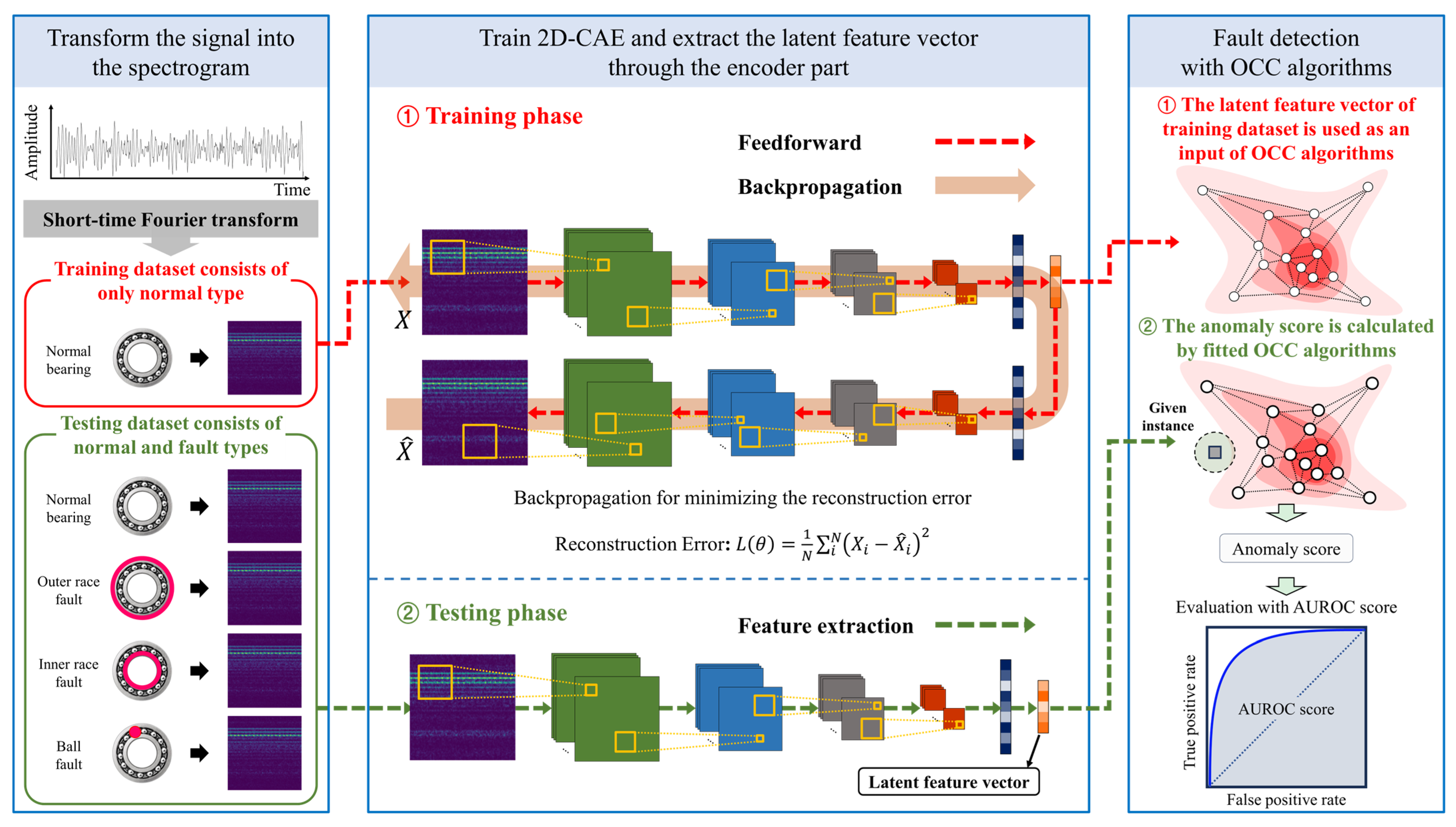
The proposed fault detection framework postulates that the fault signals are not available in the training phase. Thus, both the feature extraction and fault detection models are trained using only the signals from the normal operating state. The overall process of the proposed fault detection framework is presented in Figure 1. As shown in Figure 1, the training phase of the proposed framework comprises three subsequent procedures: (1) Firstly, raw vibration signals are obtained from the accelerometer sensors installed in the rotating machinery, and these signals are transformed into spectrograms. To this end, we applied the STFT technique to the raw time-domain vibration signals. (2) Then, a two-dimensional CAE (2D-CAE) structure is trained to reconstruct the input spectrogram obtained only from the normal operating state. In the 2D-CAE neural network, the latent feature vector is derived to summarize information on the input spectrogram. Thus, the latent feature vectors are used as extracted features of the input vibration signal in the proposed fault detection framework. (3) Finally, a fault detection model is trained with the latent feature vector of the training input spectrograms. In the fault detection model, anomaly scores of newly collected signals are computed, and those having large anomaly scores are finally rejected as fault states.

3.1. Short-Time Fourier Transform (STFT)

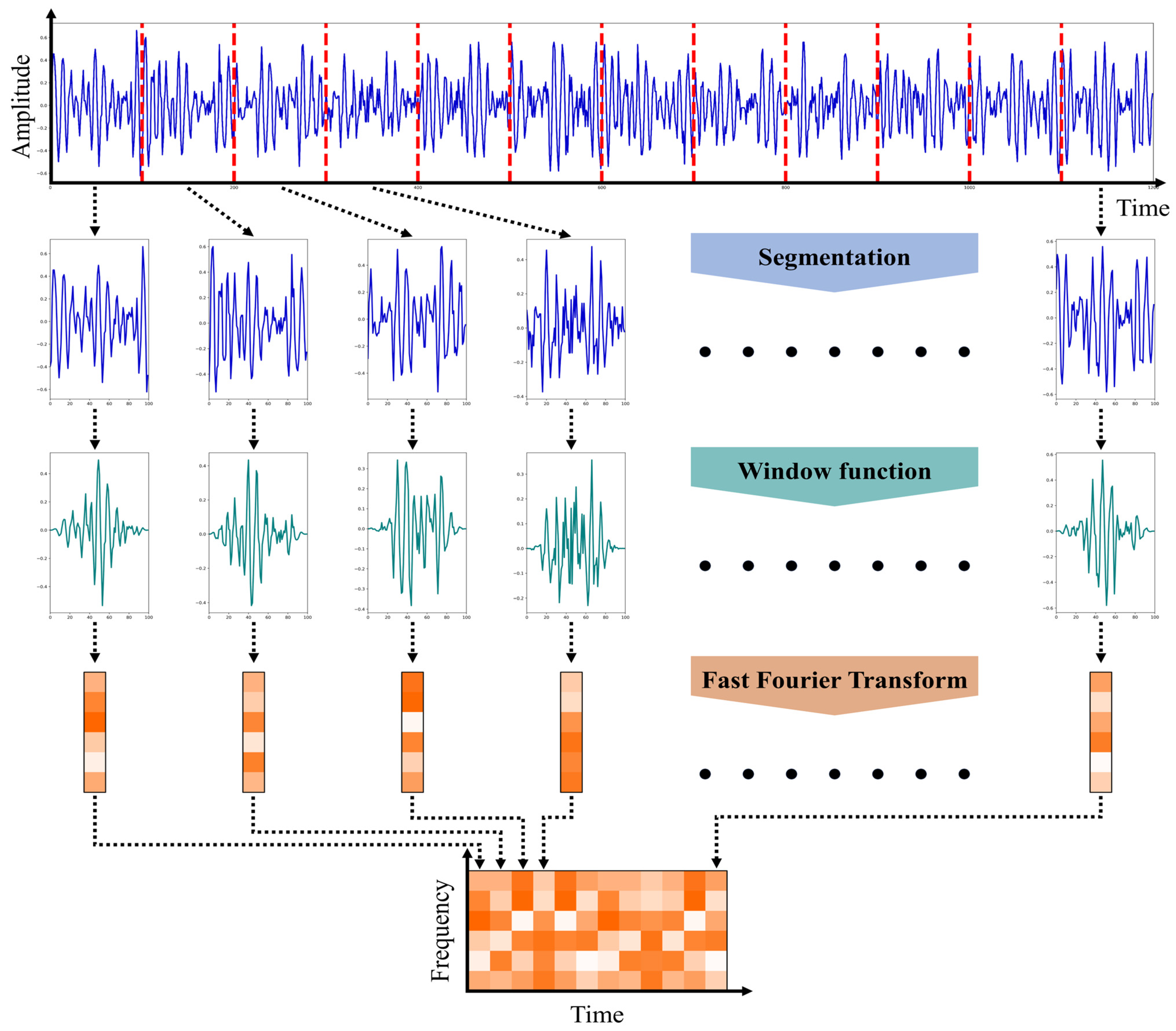
To derive the frequency information from raw time-domain signals, Fourier transform-based techniques can be adopted [60,61,62]. Among these Fourier transform-based techniques, a short-time Fourier transform (STFT) can be used to deal with the nonstationary signals. The STFT is the most widely used signal processing method for nonstationary signal analysis by capturing localized frequency properties from the signal. The STFT procedure is depicted in Figure 2. The STFT method first divides the signal into smaller consecutive segments, assuming that the signal might be locally stationary within a short time interval. However, the discontinuity at either end point of a split signal may result in the spectral leakage problem, in which the power at one frequency component erroneously leaks into other frequency components [63].

To address the spectral leakage problem, adjacent signal segments should be continuous at their end points, and thus each signal segment is multiplied with a nonzero window function whose value changes gradually toward zero at the end points. Subsequently, fast Fourier transformation (FFT) is applied to each windowed segment, and thereby, the power spectrum of each windowed segment is obtained.

The power spectrum is a representation of the power distribution across frequency components present within a windowed segment, referred to as power spectral density (PSD), and the set of spectrums of all segments comprises a spectrogram. Thus, the spectrogram provides time-frequency representation, which displays the changing patterns of frequency components over time. To this end, we firstly transform raw time-domain signals into the spectrogram by using the STFT. The continuous time signal x(t) can be transformed into a spectrum component of time t and frequency f pairs, STFT_x(t,f), as follows:

$$STF{T}_x\left(t,f\right)={\int }_{-\infty }^{\infty }x\left(\tau \right)h{\left(\tau -t\right)}^{\ast }{e}^{-j2\pi ft}d\tau ,$$

(1)

where x(τ) is the signal to be analyzed and h(τ − t) is a nonzero window function sliding over time. As for the nonzero window function, we used the Hann window function in order to mitigate the spectral leakage problem. The Hann window function, h(t), is defined as follows:

$$h\left(t\right)=0.5-0.5\cos \left({\displaystyle \frac{2\pi t}{M-1}}\right),0\le t\le M-1,$$

(2)

where M denotes the length of the signal to which the window function is applied. Then, the spectrogram is derived by taking the square of STFT_x(t,f).

$$Spectrogra{m}_x\left(t,f\right)={\left|STF{T}_x\left(t,f\right)\right|}^2={\left|{\int }_{-\infty }^{\infty }x\left(\tau \right)h(\tau -t)e^{-j2\pi ft}d\tau \right|}^2.$$

(3)

Because the collected raw time-domain signals are not completely continuous, we used the discrete STFT technique. In the discrete STFT, the discrete time signal x[n] can be transformed into a spectrum component of time point n and frequency f pairs, STFT_x(n,f), as follows:

$$STF{T}_x\left(n,f\right)=\sum _{m=-\infty }^{\infty }x\left[m\right]h[m-n]e^{-j2\pi fn},$$

(4)

where x[n] is the signal to be analyzed and h[m − n] is the window function with discrete points. Finally, the spectrogram of the discrete time signal can be obtained as follows:

$$Spectrogra{m}_x\left(n,f\right)={\left|STF{T}_x\left(n,f\right)\right|}^2={\left|\sum _{m=-\infty }^{\infty }x\left[m\right]h[m-n]e^{-j2\pi fn}\right|}^2.$$

(5)

Once the spectrogram is obtained, features of signals are extracted in the next step. The spectrogram involves information on both time and frequency, and hence, intrinsic features of raw time-domain vibration signals can be more successfully revealed. The spectrogram is represented as two-dimensional image-formatted data, and hence, we adopted the 2D-CAE model to draw meaningful features from the spectrogram in further steps.

3.2. Two-Dimensional Convolutional Autoencoder with Spectrogram

The 2D-CAE model summarizes the input spectrogram into smaller latent feature vectors through the encoder structure, and the latent feature vectors reconstruct the input spectrograms through the decoder structure. The 2D-CAE can successfully handle the spectrogram with both the convolutional and pooling layers. The convolutional layer can accommodate localized characteristics of the input data by using a convolutional kernel filter, and these convolutional kernel filters share weights across all regions of the input data. The output feature map of c-th channel in the l-th convolutional layer, $H_c^l$, is calculated as follows:

$$H_c^l=f\left(\sum _{k=1}^{C^{l-1}}{H}_k^{l-1}\ast W_{k,c}^l+b_c^l\right),c=1,2,3,\dots ,C^l,$$

(6)

where $H_k^{l-1}$ denote the output feature map of k-th channel in the (l − 1)-th layer, which is convolved with the kernel filter $W_{k,c}^l$ of c-th channel in l-th layer. $C^l$ is the number of channels in the l layer and $b_c^l$ is the bias of c-th channel in the l-th layer. In addition, $\ast$ denotes the convolutional operator and f(∙) is the activation function for a nonlinear transformation. Consequently, the output feature map having $C^l$ number of channels is obtained. Generally, each of the convolutional layers is followed by its corresponding pooling layer, integrating adjacent values of the feature map into one value. Among various pooling schemes, max-pooling, which chooses the maximum value within a local region of an input feature map, is the most widely used. By doing so, the dimensionality of feature maps and computational complexity can be considerably reduced. These convolutional and max-pooling layer pairs, referred to as a convolutional block, can be repeated multiple times. At the end of the encoder structure, the feature maps generated through multiple convolutional blocks are flattened into a one-dimensional vector and finally mapped to a latent feature vector by the fully connected layer.

Then, the input spectrogram is reconstructed from the latent feature vector in the decoder structure. The decoder structure consists of the same number of layers as the encoder structure, arranged symmetrically. That is to say, the latent feature vector is connected to a fully connected layer and reshaped into a two-dimensional feature map. The feature maps are inversely reconstructed using transposed convolutional layers and up-sampling layers instead of convolutional layers and max-pooling layers, respectively. The transposed convolutional layer, also referred to as the deconvolutional layer, enlarges the size of the input feature map as opposed to the convolutional layer in the encoder structure. The input feature map, i.e., the latent feature vector, is transformed by a transposed convolutional layer as follows:

$${\tilde{H}}_c^l=f\left(\sum _{k=1}^{C^{l-1}}{\tilde{H}}_k^{l-1}⊛{\tilde{W}}_{k,c}^l+{\tilde{b}}_c^l\right),c=1,2,3,\dots ,C^l,$$

(7)

where ⊛ stands for the transposed convolutional operator expanding the size of the input feature map. ${\tilde{H}}_k^{l-1}$ and ${\tilde{H}}_c^l$ represent the output feature map of k-th channel in (l-1)-th layer and c-th channel in l-th layer, respectively. Moreover, ${\tilde{W}}_{k,c}^l$ denotes the kernel filter of c-th channel in l-th layer and ${\tilde{b}}_c^l$ is the bias of c-th channel in l-th layer. All the parameters of the CAE are optimized by minimizing the reconstruction errors between the input data and its reconstructed outcomes. In general, the mean squared error (MSE) loss is used for the reconstruction error, which is expressed as follows:

$$MSE\left(X,\tilde{X}\right)={\displaystyle \frac{1}{N}}\sum _{i=1}^N{\left(X_i-{\tilde{X}}_i\right)}^2,$$

(8)

where X_i and ${\tilde{X}}_i$ are the i-th input spectrogram and its reconstructed one by the 2D-CAE model. In the early learning stages, the spectrogram might be poorly reconstructed because the parameters of the 2D-CAE are randomly initialized. However, as the learning process proceeds to minimize the MSE loss, the reconstructed spectrogram becomes almost similar to the original input spectrogram. In addition, the latent feature vectors summarize the more useful and concise information from the input spectrograms.

As the depth of the neural network structure increases, the internal covariate shift issue is prone to occur. To mitigate the internal covariate shift issue, we adopted a batch normalization (BN) scheme [64]. Through the use of the mean and standard deviation of the samples within a mini-batch, the BN scheme can alleviate the internal covariate shift and enhance the efficiency of training a network structure. In addition, the BN scheme helps to improve the generalization performance of DNN structures [65]. Therefore, this study applied the BN scheme as a layer into our proposed feature extractor, 2D-CAE, to improve feature extraction performance. In our proposed framework, the weights of the convolutional blocks and the fully connected layer within the 2D-CAE are trained using the Adam optimization algorithm by minimizing the MSE loss function between the input spectrogram and its reconstructed one. When the reconstruction error gets significantly low and converges to a certain level, the training procedure of the 2D-CAE is terminated.

In the 2D-CAE structure, the input spectrogram is embedded into smaller latent feature vectors by passing through multiple convolutional blocks within the encoder part, and thus, the encoder of the 2D-CAE structures can be regarded as a feature extractor. Hence, the latent feature vectors obtained from the encoder of the 2D-CAE are used as inputs of the one-class classification step. Because the 2D-CAE structure is trained with data collected only from the normal operating state, the weights of the trained 2D-CAE can incorporate information on only the normal signals. Conversely, the fault signal’s spectrogram cannot be properly involved in its latent feature vector, and the fault signal’s features might be significantly deviated from those of the normal signal.

Remark. Please note that, in the current study, the input and output of the 2D-CAE model are the same spectrograms, which are transformed from the original normal signals, not noise added. As a feature extractor, denoising the 2D-CAE model [66] can also be considered in order to deal with the intrinsic noises in the normal signals. In the denoising 2D-CAE model, the inputs of the 2D-CAE model are random noise-added spectrograms, whereas the outputs are the original spectrograms. In addition, by formulating the loss function as MSE between input and output, the latent features can capture the intrinsic properties of signals by removing the noise elements. In the current study, we conducted an experiment to compare the standard 2D-CAE (proposed) with the denoising 2D-CAE, and the comparative results are provided in Section 4. According to the comparative results, the fault detection performance of the denoising 2D-CAE is comparable to that of the original 2D-CAE. However, the denoising 2D-CAE might not be appropriate for the fault signal detection problems because the optimal level of noise added to input spectrograms is not easy to be determined. Furthermore, the standard 2D-CAE also can partially remove some of the noise because it attempts to compress the most useful features of input signals as much as possible, and the noise elements are not such informative [67]. Therefore, in this study, we propose to employ the standard 2D-CAE as the feature extractor of the input signals.

3.3. OCC Algorithm with Extracted Features from 2D-CAE for Fault Detection

After the latent feature vectors are extracted from the encoder part of the 2D-CAE, the final fault signal detection model is constructed by using OCC algorithms. The OCC algorithm builds a decision boundary solely using extracted latent feature vectors of normal signals, and the decision boundary determines whether a given signal is obtained from the normal state. If a given latent feature vector is located outside of the boundary, it is rejected as a fault, and vice versa for the vector inside the boundary. It should be noted that the normal operating patterns are well-defined, whereas the machinery fault patterns cannot be specified. Hence, the one-class classifier is constructed by only using normal signals, not relying on the information on fault signals, and it is used to discriminate between the normal signals and all other fault types. Accordingly, owing to the one-class classification, the proposed framework can be used to detect any types of faults.

In this study, we consider the most well-known OCC algorithms: Hotelling’s T² statistic, mixture of Gaussian (MoG; [18]), Parzen window density estimation (PWDE; [19]), one-class support vector machine (OCSVM; [20]), isolation forest (IsoForest; [21]), and local outlier factor (LOF; [22]). In this section, we will denote the latent feature vector extracted from the encoder part of the 2D-CAE as z and refer to the signals collected during the normal operating condition as belonging to the target class.

Hotelling’s T² statistic: It is clear that anomalous signals are located remotely from the target class region, and thus the distance from the training target class’s prototype (e.g., the mean vector of the training target class) can be considered as the anomaly level (generally referred to as the novelty score) of the newly collected samples [68,69,70]. Among various distance measures, Mahalanobis distance is the most widely used to define the novelty scores because it takes into account the correlation between features.

Hence, in this study, the novelty score is defined as the Mahalanobis distance from the mean vector of the latent feature vector z of the training target class, and this novelty score is referred to as Hotelling’s T² statistic. The Mahalanobis distance between the new signal embedded into the latent feature vector, $z_{new}$, and the mean vector of the latent features of the training target class, $\overline{z}$, $T_{new}^2$, can be defined as follows:

$$T_{new}^2={\left(z_{new}-\overline{z}\right)}^T{S}^{-1}\left(z_{new}-\overline{z}\right),$$

(9)

where S is the covariance matrix between the latent features of the training target class. The newly collected signals having larger Hotelling’s T² statistics are finally rejected as fault signals.

Mixture of Gaussian (MoG): Density measures also can be used to quantify the level of anomaly, as the anomalous samples are prone to have low density values. Among various density measures, the probability distribution function is the most widely used. To estimate the probability distribution function, mixture models are often used, which define the probability distribution function by combining multiple distributional components. The resulting mixture model is then utilized to calculate the probability distribution function of samples. MoG estimates the probability function of the target class, assuming that the target class is generated from a mixture of Gaussian probability distributions. In the MoG method, a probability distribution function of samples is represented as a weighted sum of individual Gaussian probability distribution components. Each Gaussian probability distribution component comprises its own mean vector, covariance matrix, and weight. The probability distribution function of $z_{new}$ can be computed as follows:

$$P\left(z_{new}\right)=\sum _{i=1}^K{w}_{i}P\left(z_{new}|{\mu }_i,{\Sigma }_i\right),$$

(10)

where K is the number of Gaussian probability distribution components and w_i is a weight of the i-th component. Furthermore, μ_i and Σ_i represent the mean vector and covariance matrix of the latent feature vectors in the training target class corresponding to the i-th Gaussian probability distribution component. The parameters of all Gaussian probability distribution components are estimated by maximum likelihood estimation (MLE) with the expectation maximization (EM) algorithm. Then, the signal having a high probability distribution function value is classified as a target class, and vice versa for signals with a low probability distribution function value.

Parzen window density estimation (PWDE): The PWDE is another probabilistic approach to estimate the probability distribution function of given samples. This algorithm estimates the probability distribution function through kernel functions representing the contribution of individual training samples to generate the probability distribution of the target class.

In this study, the probability distribution function of $z_{new}$, f($z_{new}$) can be described as follows:

$$f\left(z_{new}\right)={\displaystyle \frac{1}{N\sigma }}\sum _{i=1}^{N}K\left({\displaystyle \frac{z_{new}-z_i}{\sigma }}\right),$$

(11)

where N and z_i are the number of latent feature vectors of the training data and the i-th training latent feature vector, respectively. In addition, K(∙) means a kernel function, and σ denotes its bandwidth parameter. The bandwidth parameter of the kernel function plays the role of a smoothing parameter which determines the shape of the probability distribution function. A new latent feature vector having small f($z_{new}$) value is rejected as a fault signal.

One-class support vector machine (OCSVM): The support vector-based OCC algorithms directly build a decision boundary separating the majority of the target class and potential anomalous samples. The support vector-based methods attempt to involve the majority of the target class within the decision boundary, and they prevent the decision boundary from rejecting excessively large numbers of target samples as anomalies. In addition, they also employ nonlinear feature mapping into a high or infinite dimensional space, and it helps to build a flexible boundary. The most eminent support vector-based OCC algorithm is OCSVM.

In this study, the OCSVM defines the decision boundary as a hyperplane farthest from the origin, above which most of the latent feature vectors of the training target class are placed. The optimal hyperplane in the OCSVM, $w^T\phi \left(z\right)-b=0$, can be obtained by solving the following optimization problem:

$$\begin{gathered} \underset{w,\mathit{b},\mathit{\epsilon }}{\mathit{min}}{\displaystyle \frac{1}{2}}{w}^{T}w-b+{\displaystyle \frac{1}{\upsilon n}}\sum _{i=1}^n{\epsilon }_i \\ s.t.w^T\phi \left(z_i\right)-b\ge -{\epsilon }_i\forall i, \\ {\epsilon }_i\ge 0,\forall i \end{gathered}$$

(12)

where ν $\in$ (0, 1] is the hyperparameter that controls the fraction of anomalies, φ denotes a nonlinear feature mapping function, and ε_i is the slack variable of the i-th training latent feature vector z_i for allowing the soft margin. In the objective function in (12), the first term maximizes the margin, which encourages the hyperplane to enclose as many training target classes as possible. In addition, the soft margin is allowed to prevent the hyperplane from accepting too many potential fault signals as a target class. By solving its corresponding dual problem, the decision boundary can be finally derived in the form of a function $f\left(z\right)={\sum }_{i=1}^{n}K\left(z_i,z\right){\alpha }_i-b$, where α_i is the Lagrangian multiplier and K is a kernel function corresponding to the nonlinear function φ. Training latent feature vectors whose corresponding α_i is greater than zero are referred to as the support vectors, which are used to determine the decision boundary. If the new latent feature vector’s decision function value, f($z_{new}$) is a negative value, the newly collected signal is classified as a fault signal.

Isolation forest (IsoForest): IsoForest also has shown comparable performance to other existing OCC algorithms. This algorithm builds a number of isolation trees, which are constructed by randomly splitting until each terminal node contains only single (isolated) samples. The algorithm assumes that anomalous samples might be located in sparse regions and thus require only a small number of splits to isolate these sparse samples. Therefore, anomalous samples take short paths in the tree in order to reach their corresponding isolated nodes. When more isolation trees belonging to a forest generate shorter path lengths for samples, then they are more likely to be anomalies.

In this paper, the anomaly score of a new latent feature vector can be derived using the average path length to the leaf node from the isolation trees, which is expressed as follows:

$$s\left(z_{new}\right)=2^{-{\displaystyle \frac{\frac{1}{B}{\Sigma }_{i=1}^B{h}_i(z_{new})}{c\left(n\right)}}},$$

(13)

where B and n are the number of isolation trees and latent feature vectors in the training target class, respectively. Additionally, $h_i\left(z_{new}\right)$ denotes the path length to the leaf node of $z_{new}$ in the i-th isolation tree, and c(n) is the average path length of an unsuccessful search in a binary search tree and used to normalize h(∙), which is calculated as follows:

$$c\left(n\right)=2H\left(n-1\right)-\left(2\right(n-1)/n),$$

(14)

where H(∙) denotes the harmonic number and is estimated as $H\left(n-1\right)=\mathit{ln}\left(n-1\right)+0.5772156649$ (Euler’s constant). If a new latent feature vector is located in the region where the training latent feature vectors are clustered, many splits are required to isolate it, and thus the new latent feature vector will have a large anomaly score, s($z_{new}$). Conversely, latent feature vectors of the counter class (i.e., fault signals) are easily isolated with a shallow depth of the isolation tree, ultimately resulting in high anomaly scores.

Local outlier factor (LOF): The k-NN structure is a prominent data description technique that can accommodate the locality of training data. Owing to this advantage, the k-NN structures have been widely employed by OCC algorithms. Among various k-NN-based OCC algorithms, in this study, we focus on the LOF.

The LOF algorithm takes into account the local density information in anomaly score calculations. To this end, the LOF algorithm defines the local density as the average distance across neighbors of a new latent feature vector, and it calculates the anomaly score as the ratio of the average distance between $z_{new}$ and its neighbors to the local density of $z_{new}$. In this algorithm, the anomaly score of $z_{new}$, LOF($z_{new}$), is presented as follows:

$$LOF\left(z_{new}\right)={\displaystyle \frac{\sum _{i=1}^k‖z_{new}-z_i‖}{\frac{1}{\left(k-1\right)}\sum _{i,j,i\ne j}‖z_i-z_j‖}},fori,j=1,\dots ,k.$$

(15)

In the proposed fault detection framework, a latent feature vector with a large anomaly score is classified as a fault signal, while one having a small score can be regarded as a normal signal.

4. Experimental Study

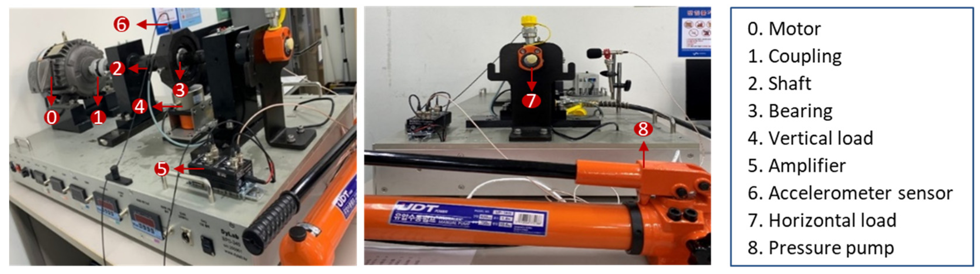
In this study, we collected vibration signals from our own rolling-element bearing experimental platform presented in Figure 3.

In this bearing experimental platform, the vibration signals were collected from the accelerometer sensor with a sampling frequency of 10,240 Hz, and the accelerometer sensor is placed on the topside of the bearing housing. In this study, vibration signals were collected by the KS94C100 accelerometer sensor, a miniature piezoelectric vibration sensor manufactured by MMF (Located in Meißner, Germany). For precise vibration measurements, it generates an IEPE (Integrated Electronics Piezo-Electric) output with a sensitivity of 10 mV/g (±5%). 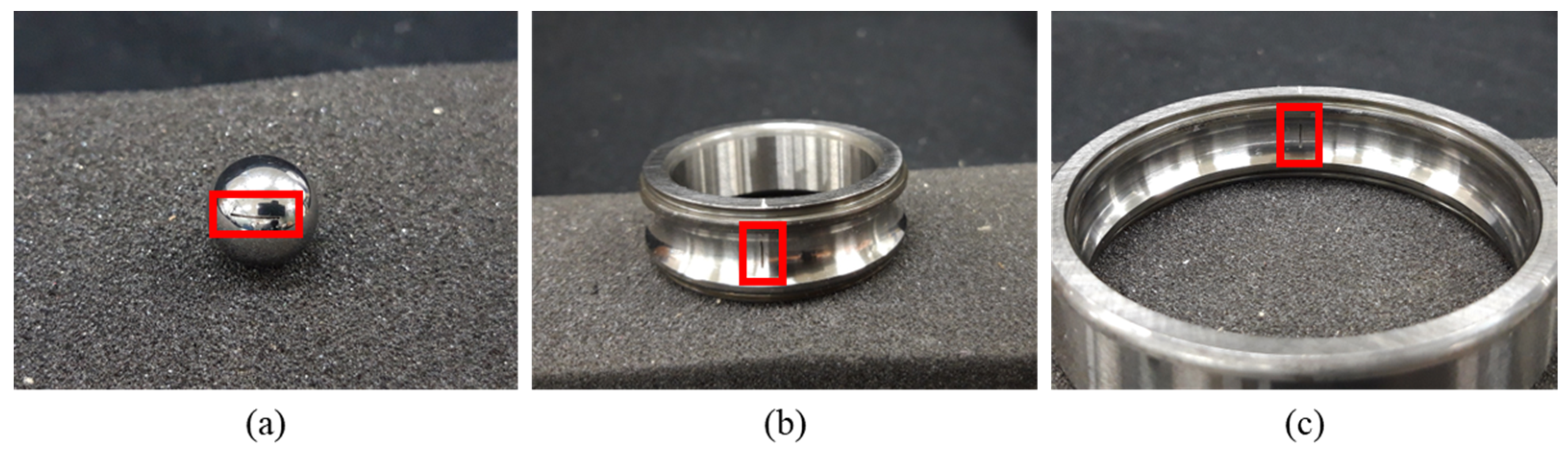The measurement range of the KS94C100 is ±60 g, corresponding to approximately ±600 m/s², and it can capture both low- and high-acceleration signals. Its frequency sampling ranges from 0.3 Hz to 28 kHz (±3 dB), ensuring accurate collection of broadband vibration signals, including high-frequency components. In the current study, a signal is collected with a length of 10,240 sampling points (i.e., a raw signal is collected per unit second). In addition, the rotating speed of the bearing is 1200 rpm (revolutions per minute), and the vertical loader presses a bearing housing with 150 kgf (kilogram-force). For the experimental platform, we used a deep-groove ball bearing of type 6207DD NSK (Manufactured from Tokyo, Japan), whose sizes of bore diameter, outside diameter, and width are 35 mm, 72 mm, and 17 mm, respectively. The signals are collected not only from a normal bearing but also from bearings having different faults which have occurred in the ball element, inner race, or outer race. These fault bearings are shown in Figure 4.

A number of previous studies regarding FDD for the bearings have also considered these three fault types because they are the most representative fault types [17,71]. Each fault at three different positions of the bearing was generated through electrical discharge machining (EDM). These three fault types are shown in Figure 4, where the fault locations are indicated by the bolded boxes. Regardless, it is known that the vibration patterns vary with fault intensity levels, and thus we also considered two fault intensity levels (i.e., strong and weak) by different defect diameters for each fault type. Consequently, the bearing state types considered in the current study are as follows: normal condition (N), strong ball element fault (SB), weak ball element fault (WB), strong inner race fault (SI), weak inner race fault (WI), strong outer race fault (SO), and weak outer race fault (WO).

To conduct all experiments, we utilized an Intel i5-9400F CPU (Intel, Santa Clara, CA, USA), NVIDIA GeForce RTX 2060 GPU (NVIDIA, Santa Clara, CA, USA), and 16 GB of RAM. All the DNN-based methods were implemented with the GPU-accelerated Pytorch (version 1.12.1) in Python (version 3.9.13). We also used the Scikit-learn library (version 1.1.1) to implement OCC algorithms. Finally, we implemented the STFT procedure using the np.fft function in the numpy library of Python (version 3.9.13).

As mentioned earlier, the training dataset consists of only normal signals, and the testing dataset is composed of the signals both in the normal operating condition and for all fault types. The number of samples for seven different bearing states is presented in

Table 2. Description of the experimental dataset.

Bearing States	Total Number of Signals
	Training Dataset	Testing Dataset
Normal condition (N)	15,680	3920
Strong ball element fault (SB)		7500
Weak ball element fault (WB)		5500
Strong inner race fault (SI)		3000
Weak inner race fault (WI)		5250
Strong outer race fault (SO)		3800
Weak outer race fault (WO)		5250

. One sample corresponds to a signal collected per second, having a length of 10,240 data points. Please note that each method is tested over 10 repetitions in order to reduce the effect of random errors.

Please note that, in this study, we did not partition the training dataset as training and validation sets because the proposed framework is basically an unsupervised learning setting. In other words, the proposed framework is available wherein the training dataset contains only normal signals, and hence, the validation procedure, which evaluates the fault detection performance, is not available in the training phase for this problem setting.

In this study, we conducted three comparative experimental studies. First, we compared different signal representation schemes: (1) time-domain representation, (2) frequency-domain representation, and (3) time-frequency domain representation (i.e., spectrogram; proposed). By doing so, we can demonstrate the advantages of the spectrogram as a signal representation for the fault detection of the rotating machinery.

In the time-domain representation scheme, the raw vibration signal having 10,240 time points is used. Meanwhile, for the frequency-domain representation, the raw vibration signal is transformed into spectral components using the SFFT. In order to preserve information on the vibration signals, the number of frequency bins is set to half of the sampling frequency (e.g., 5120 frequency points), according to the Nyquist sampling theorem [72]. Finally, we applied the STFT technique to the raw vibration signal for constructing the spectrogram. In the STFT process, the window length and hop size were carefully determined so that the spectrogram had a height and width of 128, which allows for a suitable balance between time and frequency resolution, providing a meaningful representation. For example, long windows improve the frequency resolution of the spectrogram in that they consider a wider frequency range, whereas the time resolution is degraded because the number of signal segments becomes smaller, and it is vice versa for short windows. A number of previous studies reported that there is no optimal window length suitable for any signals, but it varies depending on the signal to be analyzed. Thus, in this study, we empirically set the window length to generate a squared matrix form of the spectrogram, considering the trade-off between the time and frequency resolution. Then, 2D-CAE and one-dimensional CAE (1D-CAE) were constructed for extracting features from the spectrogram and single-domain-represented signals (time-domain- and frequency-domain-represented signals), respectively. These CAE architectures are presented in Figure 5. In this figure, values in the parentheses above each layer present their output dimensions.

As shown in Figure 5a, the encoder structure of 2D-CAE consists of four convolutional blocks, and each block comprises a convolutional layer, a max-pooling layer, a batch normalization layer, and an activation function. These convolutional blocks sequentially generate feature maps, and feature maps obtained from the fourth convolutional block are connected to the fully connected layer. In the fully connected layers, a latent feature vector with a length of 10 is derived to represent the intrinsic properties of the spectrogram. In the decoder structure, symmetric with the encoder structure, the latent feature vectors are reconstructed in the input spectrogram. In other words, the decoder structure consists of four transposed convolutional blocks substituting the convolutional and max-pooling layers of the encoder structure with the transposed convolutional and up-sampling layers, respectively. In contrast to the spectrogram, the features of single-domain-represented signals (time-domain- and frequency-domain-represented signals) are extracted through the 1D-CAE. As depicted in Figure 5b, the architecture of 1D-CAE is equivalent to that of 2D-CAE, except that it utilizes one-dimensional convolutional blocks and transposed convolutional blocks instead of two-dimensional layers.

Other hyperparameters of the CAE are represented in

Table 3. Hyperparameters of the CAE model.

Activation Function	Rectified Linear Unit (ReLU)
Learning rate	0.001
Batch size	256
Epoch	50

.

As shown in Table 3, we used the ReLU function as an activation function because it is the most widely employed one for the CAE. The ReLU simply outputs zero for negative inputs and a linear identity for positive ones. By doing so, it can reflect nonlinearity and enhance computation efficiency. Furthermore, this activation function helps parameters of CAE to converge faster during training and alleviates the vanishing gradient problem. In addition to the activation function, we set other hyperparameters, learning rate, batch size, and epoch to be specified as 0.001, 256, and 50, respectively. It is known that the performance of the neural network is not affected by those hyperparameters; we simply set them as the default recommended ones in the open library.

In this study, we presented the time-domain-represented signals, frequency-domain-represented signals, and spectrograms of raw signals of all bearing conditions as in Figure 6, Figure 7 and Figure 8. The frequency domain representations are obtained by applying fast Fourier transformation (FFT) to raw time-domain signals, and spectrograms are also obtained by applying short-time Fourier transformation (STFT) to raw time-domain signals.

As shown in Figure 6, Figure 7 and Figure 8, the frequency-domain-represented signals and spectrograms more clearly represent the difference between normal and other fault bearings than time-domain-represented signals. Furthermore, in the spectrogram, each bearing condition differs more than other single-domain-represented signals. These figures indicate that spectrograms can achieve more accurate fault detection performance than single-domain-represented signals.

In addition, we also visualized these 10 latent features by facilitating the t-distributed stochastic neighborhood embedding (t-SNE; [73]) technique. Figure 9 shows the two-dimensional t-SNE plots of latent features obtained from each signal representation scheme.

Figure 6, Figure 7, Figure 8 and Figure 9 demonstrate that the frequency-domain information is more helpful for discriminating between the normal signals and fault ones in that the normal signals are more clearly separated from fault signals (Figure 9b,c). A one-dimensional time-domain signal provides insufficient information on the operating state of rotating machinery in that the time-domain signal is significantly confounded by environmental noise, which cannot be fully removed in many real situations. Therefore, using only time-domain representation cannot accurately detect the ball element fault from the normal signals, and other fault types have also overlapped each other. On the other hand, although the frequency information is more useful than time-domain information regarding fault signal detection, the normal signals are slightly overlapping with the ball element fault types in solely using the frequency information case (Figure 9b). It should be noted that the frequency information cannot be properly derived from nonstationary signals, which are often encountered in many real situations. In contrast to single-domain signal representation schemes, the use of spectrograms most clearly distinguishes the normal signals and other fault types. Additionally, all fault types are also well separated, even without utilizing the label information of fault types. Because the spectrogram can deal with the nonstationary signals by applying the FFT technique to stationary signal segments, the frequency information can be more precisely derived. This visualization result indicates that the spectrogram can represent the meaningful characteristics of the operating state of rotating machinery and symptoms of machinery faults.

In addition to visual comparison, we used the area under the receiver operating characteristic curve (AUROC) to compare the fault detection performance of three signal representation schemes. In fault detection problems, the receiver operating characteristic (ROC) curve is used to display the trade-off relationship between two types of errors, namely, the true positive rate and false positive rate. The true positive rate is the rate of true fault signals, which are correctly classified as fault signals, while the false positive is the rate of true normal signals, which are incorrectly classified as faults. When the threshold value for the anomaly score is large, it results in a high false-positive rate and a low true-positive rate, whereas a small threshold value leads to a low false-positive rate and a high true-positive rate. The ROC curve is obtained from both the true positive rate and false positive rate from all possible thresholds. The AUROC score is defined as the area under the ROC curve, and the larger AUROC score implies the better fault detection performance. Because the AUROC score does not rely on threshold setting, it is the most widely used evaluation measure for the fault detection problems [74]. To compute the AUROC score, we used the six OCC algorithms as fault detectors, which are Hotelling’s T² statistic, MoG, PWDE, LOF, OCSVM, and IsoForest.

The hyperparameters of the OCC algorithms are not easy to be optimize due to the absence of counter-class information [75]. Therefore, the hyperparameters of those six OCC algorithms were specified as default values suggested by the Scikit-learn library, and these default values have shown reasonable fault detection performance.

Table 4. Average AUROC values from three different signal representation schemes with CAE and six OCC algorithms.

Signal Representations	Hotelling’s T2 Statistic	MoG	PWDE	OCSVM	IsoForest	LOF
Time-domain + 1D-CAE	0.608	0.609	0.608	0.656	0.638	0.790
Frequency-domain + 1D-CAE	0.853	0.853	0.799	0.720	0.823	0.930
Spectrogram + 2D-CAE (Proposed)	0.966	1.000	0.942	0.831	0.907	1.000

The largest AUROC values are represented in bold and underline.

shows AUROC values of each signal representation scheme using the six OCC algorithms. In this table, we reported the average AUROC values obtained from 10 repetitions.

The results in Table 4 indicate that, across all OCC methods, using the spectrogram yielded larger AUROC values compared to single-domain signal representation schemes, clearly demonstrating its superiority over the others. Hence, in further experimental studies, we used the spectrogram as a signal representation scheme.

In addition, we also compared four feature extraction methods for the fault detection: (1) using manually defined features, (2) principal component analysis (PCA), (3) kernel PCA, (4) stacked autoencoder (stacked AE), (5) denoising two-dimensional convolutional autoencoder (denoising 2D-CAE), and (6) standard 2D-CAE (proposed). As for the manually defined features, we computed 10 statistics from the signal in both the time and frequency domains. They are the most widely used in previous signal preprocessing studies [24,76].

Table 5. Summarization of 10 manually defined features considered in this study.

	Features	Definition
Time-related features	Root mean square	$T_{rms}={\left[{\displaystyle \frac{1}{n}}{\displaystyle \sum _{i=1}^n}{x}_i^2\right]}^{{\displaystyle \frac{1}{2}}}$
	Skewness	$T_{sk}={\displaystyle \frac{\sum _{i=1}^n{\left(x_i-\overline{x}\right)}^3}{\left(n-1\right){\sigma }^3}}$
	Kurtosis	$T_{ku}={\displaystyle \frac{\sum _{i=1}^n{\left(x_i-\overline{x}\right)}^4}{\left(n-1\right){\sigma }^4}}$
	Crest factor	$T_{cf}={\displaystyle \frac{x_{max}}{x_{rms}}}$
	Shape factor	$T_{sf}={\displaystyle \frac{T_{rms}}{\overline{x}}}$
	Impulse factor	$T_{if}={\displaystyle \frac{x_{max}}{\overline{x}}}$
Frequency-related features	Mean frequency	$F_{mf}={\displaystyle \sum _{i=1}^N}{\displaystyle \frac{p_i}{N}}$
	Frequency center	$F_{fc}={\displaystyle \frac{\sum _{i=1}^N{f}_i{p}_i}{\sum _{i=1}^N{p}_i}}$
	Root mean square frequency	$F_{rmsf}={\left[{\displaystyle \frac{\sum _{i=1}^N{f}_i^2{p}_i}{\sum _{i=1}^N{p}_i}}\right]}^{{\displaystyle \frac{1}{2}}}$
	Root variance frequency	$F_{rvf}={\left[{\displaystyle \frac{\sum _{i=1}^N{\left(f_i-F_{mf}\right)}^2{p}_i}{\sum _{i=1}^N{p}_i}}\right]}^{{\displaystyle \frac{1}{2}}}$

summarizes the manually defined features considered in the current study. In Table 5, x is the time-domain signal to be analyzed, and n is the length of the signal. Furthermore, the absolute mean value of the time-domain signal is represented as $\overline{x}$, and $x_{max}$ denotes the maximum value in a signal. For frequency-related features, N is the number of frequency bins, and f_i denotes the frequency value of the i-th bin. Additionally, p_i corresponds to the amplitude of the i-th spectrum component.

In addition, for the kernel PCA, we adopted the radial basis function (RBF), whose bandwidth (σ) is one, as a kernel function. Finally, the noise added to the spectrogram is generated from the Gaussian distribution, whose mean value is 0 and standard deviation is 0.1, because excessively large noises might deteriorate the patterns of the spectrogram, and the deteriorated spectrogram cannot generate appropriate latent features of input signals.

In this comparative study, the spectrogram is used as the input for feature learning methods, except for the manually defined feature method. For the PCA and AE, each element of the spectrogram is regarded as a single variable. Thus, the spectrogram is transformed into a one-dimensional vector of length 16,384 from a square matrix of order 128. The spectrogram, a two-dimensional matrix, is directly used as the input for the 2D-CAE. For a fairer comparison with the manually defined features, we extracted 10 features for each feature learning method. Then, we applied the six OCC algorithms to the 10 extracted features for the fault detection.

Table 6. AUROC values for the different feature extraction methods with the spectrogram and six OCC algorithms.

Signal Representations	Hotelling’s T2 Statistic	MoG	PWDE	OCSVM	IsoForest	LOF
Manually defined features	0.882	0.966	0.870	0.834	0.847	0.975
Spectrogram + PCA	0.902	0.994	0.970	0.910	0.898	0.997
Spectrogram + Kernel PCA	0.895	0.982	0.970	0.904	0.884	0.997
Spectrogram + Stacked AE	0.938	0.998	0.917	0.851	0.867	0.993
Spectrogram + Denoising 2D-CAE	0.962	0.997	0.912	0.842	0.876	0.989
Spectrogram + standard 2D-CAE (Proposed)	0.966	1.000	0.942	0.831	0.907	1.000

The largest AUROC values are represented in bold and underline.

presents AUROC values of each feature extraction scheme using six OCC algorithms.

As presented in Table 6, the 2D-CAE tends to achieve the best or comparable performance among all feature extraction methods. Since the convolutional blocks, composed of convolutional and max-pooling layers, help to recognize local patterns from the image-formatted data, the 2D-CAE can successfully extract informative features from the spectrogram. In contrast, the manually defined features cannot demonstrate superior performance, as they are computed using simple statistics and fail to reflect the intrinsic properties of complicated signal data. PCA-based feature extraction also tends to yield worse performance than the 2D-CAE because PCA cannot adequately accommodate the nonlinearity inherent in the input distribution of spectrograms. In addition, PCA handles the elements of the spectrogram as individual features, which hinders the successful recognition of localized characteristics within the spectrogram. While the stacked AE can deal with the nonlinear patterns through nonlinear activation functions, it still cannot capture the localized properties of the spectrogram, the same as the PCA and kernel PCA. On the other hand, the fault detection performance of the denoising 2D-CAE is comparable to that of the original 2D-CAE because it can properly deal with the noise in signals. However, this DNN-based method might not be appropriate for the fault signal detection problems because the optimal level of noise added to the spectrogram is not easy to determine. Furthermore, standard 2D-CAE can also partially eliminate some of the input noise [67]. Therefore, we suggest using 2D-CAE as the feature extraction method for fault detection with the spectrogram. In these comparative results, the PWDE and OCSVM algorithms perform better in the PCA-based feature extraction scheme. These two methods are based on the kernel function, and they can accommodate the nonlinear structures of the normal signals. This property works well in the latent features obtained from linear feature extraction methods, such as PCA. On the other hand, in latent features obtained from other DNN-based feature extraction methods, the nonlinearity of the normal signals is already accommodated, and the kernel function-based one-class classification methods might not be effective.

The experimental results in Table 4 and Table 6 also provide noteworthy implications regarding the OCC algorithms as a fault detector within the proposed framework. As shown in these results, the LOF and MoG generally achieved the first and second highest performance because they can consider the local patterns of extracted features. That is to say, these two OCC algorithms can construct more sophisticated decision boundaries, and this helps to accommodate the complicated patterns within the extracted features obtained from any signal representation schemes or feature extraction methods. It should be noted that the vibration signals obtained from the real-world rotating machinery might generate noisy vibration signals corrupted by sampling errors or the interference of uncontrollable physical factors [15,16]. The extracted features obtained from these corrupted vibration signals also might be noisy, and it eventually leads to an unsatisfactory fault detection performance by the OCSVM and IsoForest algorithms. For example, in the case of OCSVM, the support vectors are often selected around the outer side of normal signal structures, which could potentially include noisy normal signals. As a result, the final decision boundary of the OCSVM is susceptible to the influence of noise or outliers, leading to a poor fault detection performance [70,77]. The IsoForest algorithm also yielded lower AUROC scores, likely due to its sensitivity to the noisy patterns. When dealing with a noisy target class, the individual isolation trees tend to generate too many unnecessary splits. These undesirable splits within the individual isolation trees result in poor anomaly score computation by the IsoForest algorithm. Hence, the IsoForest algorithm fails to achieve superior fault detection performance.

In this experiment, we also compared the proposed fault detection framework with other deep neural network-based fault detection methods, including reconstruction error of the SAE (ReSAE) and the 2D-CAE (ReCAE), deep support vector data description (Deep SVDD), and anomaly detection with generative adversarial network (AnoGAN). For all these fault detection methods, the spectrogram was used as input. In addition, for a fairer comparison, the Deep SVDD and the AnoGAN algorithms are implemented with the CNN as a base network structure, and the CNN structures of these two algorithms have the same number of convolutional blocks as the proposed fault detection framework. The AUROC values of these fault detection methods are presented in

Table 7. AUROC values of six deep neural network-based fault detection methods.

Deep Neural Network-Based Fault Detection Methods	AUROC
ReSAE	0.625
ReCAE	0.923
Deep SVDD	0.926
AnoGAN	0.645
2D-CAE + MoG (Proposed)	1.000
2D-CAE + LOF (Proposed)	1.000

The largest AUROC values are represented in bold and underline.

.

As presented in Table 7, the 2D-CAE with the MoG and LOF outperforms other deep neural network-based methods considered in the current study. On the other hand, when compared to the ReSAE, the ReCAE performs better because the convolutional block in the CAE helps to successfully handle the image-formatted spectrogram. However, those anomaly scoring methods, ReSAE and ReCAE, show undesirable performance because the reconstruction error between the input spectrogram and its reconstructed outcomes cannot properly quantify the level of fault in the signals. The Deep SVDD algorithm also fails to achieve superior performance even though the decision boundary is created in an end-to-end manner. The training procedure of Deep SVDD was designed to minimize the distance between the center of the hypersphere and normal signals in the latent feature space. However, this approach is basically related to support vector-based OCC algorithms, and hence, it is also sensitive to the noisy signals. That is to say, the Deep SVDD algorithm only focuses on reducing the volume of the hypersphere enclosing all training target classes, and the hypersphere is distorted due to a couple of noise latent feature vectors corresponding to the noisy training signals. On the other hand, because the AnoGAN is based on the generative model, this method also suffers from the mode collapse problem, which is a critical limitation of the generative model. That is to say, artificial spectrograms created by a generator only resemble the prototype spectrogram obtained from the normal states, and they cannot fully depict the elaborate patterns to discriminate between normal and fault states. Consequently, the AnoGAN method achieved poor fault detection performance.

5. Conclusions

In this study, we propose a framework for detecting faults in rotating machinery without signals obtained from the rotating machinery in fault states. The main contributions of the proposed framework can be summarized as follows: (1) Owing to the STFT-based spectrogram, information on time-varying patterns of frequency components can be revealed. By doing so, intrinsic properties of noisy and nonstationary signals can be successfully utilized for fault detection on rotating machinery. (2) In addition, by applying the 2D-CAE as a feature extractor, more informative latent features from two-dimensional spectrograms can be extracted in that the convolutional blocks in CAE are specialized to generate features from the image-formatted data. (3) Finally, the OCC algorithm helps to build an elaborate decision boundary under the situations wherein counter classes (i.e., fault signals) are not available, which is frequently encountered in many real industrial fields.

In the current study, we first transformed the raw time-domain vibration signal into a spectrogram using the STFT technique in order to represent both time and frequency characteristics. Then, the 2D-CAE was trained to embed the spectrogram into a much smaller latent feature vector. These latent vectors can be obtained by passing through several convolutional blocks within the encoder part of the 2D-CAE, and thus, the encoder of the CAE structures can be used as a feature extractor. Finally, by solely using the extracted latent feature vectors of the normal signals, fault detectors were trained by OCC algorithms, and the fault detector determined whether newly collected signals were generated from a normal state. To demonstrate the efficacy of the proposed fault detection framework, we used the rolling bearing experimental platform, which generates the vibration signals with accelerometer sensors. The comparative experiments demonstrated that our proposed framework achieved the highest AUROC score for bearing fault detection based on vibration signals. In this study, we released whole source codes to implement the experimental studies in the open-source repository (https://github.com/BAP-SAE/FD_CAE_Spectrogram; accessed on 6 July 2025). We believe that this uploaded source code can guarantee the reproducibility and replicability of the proposed fault detection framework with the spectrogram and 2D-CAE model.

In the future, we will extend the proposed fault detection problems to other rotating machinery systems. Because vibration signals are generally collected from other types of machinery systems, including electric motors and aircraft turbine engines, we believe that the proposed framework can also be applied to fault detection tasks for any rotating machinery systems. Besides, we will apply the proposed framework to the detection of various other fault types. In particular, we will extend the proposed fault detection framework for degradation faults (rust faults, abrasion faults, and scratches), which are not easy to accurately detect. Because of the one-class classification, the proposed framework can successfully detect these types of faults.