Sensitivity Estimation for Differentially Private Query Processing

Abstract

Differential privacy is a robust framework for private data analysis and query processing, which achieves privacy preservation by introducing controlled noise to query results in a centralized setting. The sensitivity of a query, defined as the maximum change in query output resulting from the addition or removal of a single data record, directly influences the magnitude of noise to be introduced. Computing sensitivity for simple queries, such as count queries, is straightforward, but it becomes significantly more challenging for complex queries involving join operations. In such cases, the global sensitivity can be unbounded, which substantially impacts the accuracy of query results. While existing measures like elastic sensitivity and residual sensitivity provide upper bounds on local sensitivity to reduce noise, they often struggle with either low utility or high computational overhead when applied to complex join queries. In this paper, we propose two novel sensitivity estimation methods based on sampling and sketching techniques, which provide competitive utility while achieving higher efficiency compared to existing state-of-the-art approaches. Experiments on real-world and benchmark datasets confirm that both methods enable efficient differentially private joins, significantly enhancing the usability of online interactive query systems.

1. Introduction

In modern data-driven applications, join operations are widely used in areas ranging from social networking analysis [1,2] to healthcare information management [3,4], enabling the combination of datasets to reveal valuable insights and facilitate decision-making. However, this widespread use also introduces significant privacy risks. Sensitive information, such as personal records, can be exposed through vulnerabilities in third-party servers [5,6], leading to potential misuse and violations of individual privacy. As a robust framework for privacy-preserving data analysis, differential privacy (DP) [7] introduces controlled noise to query results, ensuring that individual data contributions remain indistinguishable, thereby safeguarding data privacy. Usually, the noise is determined by the sensitivity [8], defined as the maximum difference in query results between two datasets differing by one record. Traditional sensitivity measures, such as global sensitivity, are easily applied to single-table queries, and the refined versions, such as local sensitivity and smooth sensitivity [9], are similarly applicable. However, for join queries, these methods prove inadequate, as they either introduce unbounded sensitivity or result in prohibitively intensive computation.

Recent studies have proposed elastic sensitivity (ES) [10] and residual sensitivity (RS) [11] based on the upper bound of local sensitivity to achieve optimal performance in specific settings, but these methods still have certain limitations. First, residual sensitivity suffers from computational inefficiency when processing large-scale complex join queries. Second, since elastic sensitivity always considers the worst case, it tends to overestimate sensitivity, resulting in degraded data utility. Existing work lacks a sensitivity calculation method that balances efficiency and utility. Therefore, this paper will investigate this aspect to address the challenges.

Our observation is that the query sensitivity is typically computed based on certain database statistics, with more accurate sensitivity requiring increasingly complex and time-consuming statistical calculations. To tackle this problem, we raise the idea of using approximate query processing (AQP) methods to estimate query sensitivity. We present a sensitivity estimation framework, as illustrated in Figure 1. While we focus specifically on sensitivity estimation for multi-way join queries in this study, this core idea can be extended to a wide range of query types.

To address the efficiency issue in the calculation of residual sensitivity. We propose Sampling-SE, which approximates the maximum boundary of each residual query using a sampling-based method, RQE. Specifically, it estimates the frequencies of the maximum groups in the residual queries of a multi-join query via random walks. To address the utility issue in the use of elastic sensitivity, we propose Sketch-SE with sketching sensitivity, which is defined based on the AGMS sketch [12]. Since sketches for the relations involved in join queries are constructed offline, they can be used to efficiently estimate sensitivity when a query arrives. The main contributions of this paper are as follows:

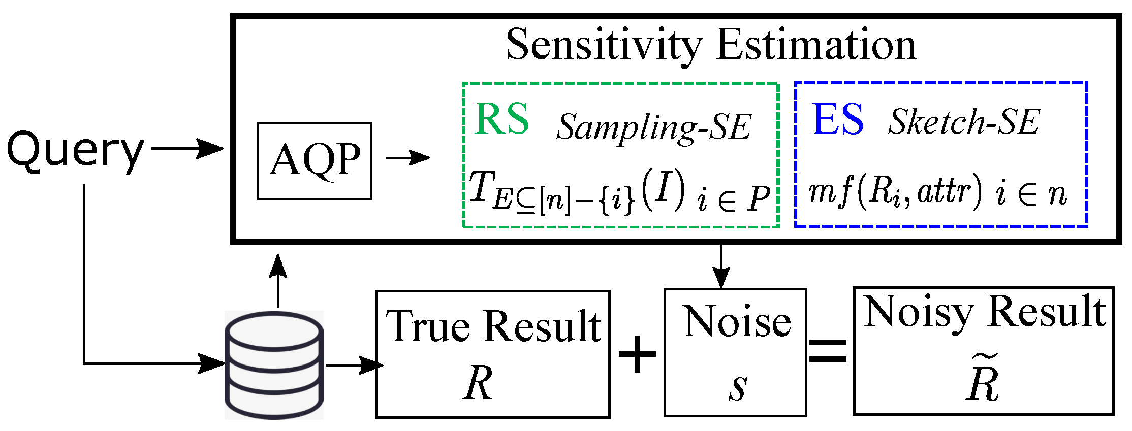
• We present a sampling-based sensitivity estimation method called Sampling-SE for differentially private join query processing, which improves the efficiency of calculating residual sensitivity while remaining comparable in terms of accuracy;
• We also present a sketch-based method called Sketch-SE using sketching sensitivity, which improves the utility of elastic sensitivity while remaining highly efficient;
• Experimental results on real-world and benchmark datasets show that our proposed methods obtain better performance than the traditional implementation of RS and ES.

The remainder of the paper is organized as follows. We review the related work in Section 2. In Section 3, we introduce the preliminaries of differential privacy and the existing definitions of sensitivity. Section 4 introduces two sensitivity estimation methods for multi-join queries based on sampling and sketches. In Section 5, we present experimental comparisons of our methods and existing ones. Section 6 concludes the paper.

2. Related Works

Differential Privacy [7] is a mathematical framework aiming at quantifying and managing privacy risks. It is widely used in the field of privacy-preserving data releasing [13,14] and mining [15,16], machine learning [17,18], and social network analysis [19]. Differential privacy can be easily applied to protect the privacy of query processing by adding noise correlated to the sensitivity into the query results [8], gaining traction in many real-world applications [20,21].

Computing the sensitivity of join queries is challenging. Recently, several mechanisms supporting join queries have been proposed, such as Privacy Integrated Queries (PINQs) [22] and its weighted version wPINQ [23], but both of these are based on global sensitivity, which means that the sensitivity could be extremely large, thus resulting in low utility. Nissim et al. [9] propose local sensitivity to fix one of two datasets that are adjacent to the actual dataset being queried and take into account all its neighbors. However, it does not meet the requirements of differential privacy. Smooth sensitivity [9] is the tightest smooth upper bound of local sensitivity that can prevent the privacy leakage caused by the mutation of local sensitivity, but its computation complexity is Non-deterministic Polynomial-time hard (NP-hard). Elastic sensitivity (ES) [10] and residual sensitivity (RS) [11] are both based on the idea of finding the smooth upper bound of the local sensitivity. ES is computed based on the maximum frequency of the join values in each relation, and RS is computed based on some residual queries of a multi-join query.

Approximate query processing (AQP) is a technique that can be used to estimate join sizes efficiently [24]. Sampling [25,26] the join result is one of the AQP methods that has high performance. Ripple join [27] and wander join [28] are online aggregations that can be used for queries with join operators. Zhao et al. [29] revisited this issue to integrate the previous approaches into a universal framework that contains two main phases: calculating the upper bound of the join size weight and then sampling from the joins. Moreover, there are other techniques, such as histograms [30,31], that are leveraged to estimate the size of join query results. AQP presents a viable solution for efficient and private data analysis [32,33], particularly when exact query answers cannot be obtained under DP constraints. Sketches are probabilistic data structures used for stream summarization tasks, and masses of sketches, such as AGMS [12,34], Count-sketches [35], and Count-Min sketches [36], are proposed for frequency estimation, heavy hitter mining, join size estimation, etc. AGMS sketch is designed for self-join estimation, which can also be used to estimate the join size of multi-join queries, including condition filters [37]. Zhang et al. [38] introduce a join size estimation framework under LDP based on FAGMS sketch [39].

Although a variety of definitions for sensitivity are proposed for join queries, they all have some shortcomings. Global sensitivity is unbounded for multi-join queries, and local sensitivity does not satisfy the differential privacy. The computation of smooth sensitivity is NP-hard. ES is easy to compute but has poor accuracy. RS is more accurate but more time-consuming. No existing studies have made efforts toward adopting AQP methods for sensitivity estimation. However, AQP methods such as sampling and sketches cannot be simply adopted to reduce the cost. This is because the sensitivity of a multi-join query depends on many statistics, as shown in RS, and individually estimating each statistic is still costly. Therefore, we propose a sampling-based sensitivity estimation method to focus on estimating the statistics and how this contributes to the sensitivity. We also propose a sketch-based method that constructs sketches for each relation offline and efficiently estimates the sensitivity online.

3. Preliminaries

In this section, we introduce some definitions of differential privacy and different kinds of sensitivity. The notations used in this section are defined in Abbreviations.

3.1. Differential Privacy

Differential privacy [7] ensures that any individual in or not in the dataset has little effect on the final released query results.

Definition 1.

$(ϵ,\delta )$-Differential privacy. A randomized privacy algorithm A satisfies ϵ-DP if for any pairs of input datasets, I and $I^{\prime }$ satisfy $d(I,I^{\prime })=1$ for all sets S of possible outputs.

$$Pr[A(I)\in S]\le exp(ϵ)·Pr[A(I^{\prime })\in S]+\delta$$

(1)

ϵ denotes the privacy budget, indicating the degree of privacy protection.

Theorem 1. 

Laplace mechanism [8]. Given a dataset I, function f:$I\to R^d$. So, the random algorithm $A:A(I)=f(I)+Y$ provides ϵ-differential privacy protection, and $Y\sim Lap(△f/ϵ)$ presents the randomized noise, which follows a Laplace distribution with scale parameter $△f/ϵ$. The factor $△f$ represents sensitivity.

3.2. Sensitivity

Sensitivity measures the maximum change in the query result when inserting or deleting a record. In this section, we introduce five different definitions of sensitivity. Global sensitivity calculates the maximum difference of the query result on two neighboring databases, i.e., $d(I,I^{\prime })=1$.

Definition 2. 

Global sensitivity (GS) [8]. For $q:D^n\to R^d$ and all $I,I^{\prime }\in D^n$, the GS of q is

$$G{S}_q=\underset{I,I^{\prime }:d(I,I^{\prime })=1}{max}\left|\right|q(I)-q(I^{\prime })\left|\right|$$

(2)

Local sensitivity is defined similarly, but computed for a fixed database.

Definition 3. 

Local sensitivity (LS) [9]. For $q:D^n\to R^d$ and $I^{\prime }\in D^n$, the LS for I is

$$L{S}_q(I)=\underset{I^{\prime }:d(I,I^{\prime })=1}{max}\left|\right|q(I)-q(I^{\prime })\left|\right|$$

(3)

However, local sensitivity poses privacy risks. To address this, smooth sensitivity is proposed to compute a smooth upper bound on local sensitivity.

Definition 4. 

Smooth sensitivity [9]. Smooth sensitivity is defined based on the generalization of the local sensitivity of f at distance k,

$$L{S}_q^k(I)=\underset{I^{\prime }\in D^n:d(I,I^{\prime })=k}{max}L{S}_q(I^{\prime })$$

(4)

and the smooth sensitivity of q for I is

$$S{S}_q(I)=\underset{0\le k\le n}{max}{e}^{-\beta k}L{S}_q^k(I),\beta ={\displaystyle \frac{ϵ}{2ln2/\delta }}$$

(5)

Computing smooth sensitivity is time-consuming, requiring exponential time for large datasets. To address this, elastic and residual sensitivities are proposed, both of which are smooth upper bounds of local sensitivity. Nissim et al. [9] proved that any smooth upper bound of local sensitivity can preserve privacy according to differential privacy.

Definition 5. 

Elastic sensitivity [10]. The elastic sensitivity of a database I is defined based on the smooth upper bound of local sensitivity as follows.

$$E{S}_q(I)=\underset{0\le k\le n}{max}{e}^{-\beta k}{\widetilde{LS}}_q^k(I),\beta ={\displaystyle \frac{ϵ}{2ln2/\delta }}$$

(6)

where ${\widetilde{LS}}_q^k(I)$ is an upper bound of local sensitivity at distance k,

$$\begin{array}{c}\hfill {\widetilde{LS}}_q^k(I)=\underset{i\in P}{max}(\prod _{j\in P-\left\{i\right\}}(mf(x_j\cap x_{p(j,i)},I_j)+k)·\prod _{j\in [n]-P}mf(x_j\cap x_{p(j,i)},I_j))\end{array}$$

(7)

$mf(x,I_j)$ is the maximum frequency on attribute x in $I_j$, and P is the private attribute set.

Elastic sensitivity can be computed based on the maximum frequencies of the join attributes. However, it computes the maximum frequency of the multi-way join based on the assumption that all of the most frequent join attribute values can be joined with each other. So, elastic sensitivity involves many errors.

Definition 6. 

Residual sensitivity [11]. The residual sensitivity of a database I is also defined based on the smooth upper bound of local sensitivity at distance k,

$$R{S}_q(I)=\underset{0\le k\le n}{max}{e}^{-\beta k}min(\widehat{G{S}_q},{\widehat{LS}}_q^k(I)),\beta ={\displaystyle \frac{ϵ}{2ln2/\delta }}$$

(8)

where ${\widehat{LS}}_q^k(I))$ is an upper bound of local sensitivity at distance k,

$${\widehat{LS}}_q^k(I)=\underset{s\in S^k}{max}\underset{i\in P}{max}{\widehat{T}}_{[n]-\left\{i\right\},s}(I)$$

(9)

$${\widehat{T}}_{E,s}(I)=\sum _{E^{\prime }\subseteq E}\left(T_{E-E^{\prime }}(I)\prod _{i\in E^{\prime }}{s}_i\right)$$

(10)

${\widehat{T}}_{E,s}(I)$ computes the maximum boundary for $I^{\prime }:d(I,I^{\prime })=k$, and s is one way of partitioning k into different relations in E.

Residual sensitivity requires computing the maximum boundaries of residual queries for each private relation. This involves solving a join-aggregate query with group-by conditions, which remains computationally expensive, especially for complex joins.

4. Sensitivity Estimation for Join Queries

In this section, we propose two sensitivity estimation methods based on sampling and sketch, respectively. The notations in this section are shown in Abbreviations.

4.1. Limitation of Existing Sensitivity Measures

This subsection is derived from the previous sections. Prior to presenting our sensitivity estimation methods, we first revisit existing exact sensitivity computation methods in previous work. For instance, the sensitivity of “SELECT Count(*) FROM data WHERE Salary > 5000;” is 1, as modifying one record affects the result by, at most, 1. However, join queries present greater complexity, since a single record change may significantly impact the query results. Consider query q = $Count(R_1(A,B)\bowtie R_2(B,C)\bowtie R_3(C,D))$ on the relations shown in Figure 2; calculating its sensitivity while maintaining privacy, accuracy, and efficiency is challenging. Current solutions like ES and RS use the smooth upper bound of local sensitivity, yet they still face accuracy and efficiency limitations.

A join query q = $Count(R_1(A,B)\bowtie R_2(B,C)\bowtie R_3(C,D))$ is shown in Figure 2. ES and RS use different ways to compute the upper bound of the local sensitivity when deleting or inserting a tuple into the relations.

(1) ES calculates the upper bound based on the maximum frequency of each join attribute as follows:

$$\begin{array}{cc}\hfill max& (mf(R_1.B)·mf(R_2.C)\hfill \\ \hfill & mf(R_1.B)·mf(R_3.C)\hfill \\ \hfill & mf(R_2.B)·mf(R_3.C))\hfill \end{array}$$

Here, $mf(X)$ denotes the most-frequent value frequency of attribute X. The product $mf(R_1.B)·mf(R_2.C)$ gives the upper bound for attribute C’s frequency in $R_1\bowtie R_2$. The worst-case sensitivity occurs when each tuple in $R_2$ with the most frequent value for $(R_2.C)$ also contains the attribute value $(R_2.B)$, matching the most frequent value of $(R_1.B)$. However, as shown in Figure 2, reality often differs from this worst-case scenario. Here, $(R_1.B)$’s most frequent value $b_1$ doesn’t match the most frequent value $c_2$ of $(R_2.C)$. Therefore, the upper bound is much higher than the actual influence of inserting or deleting a tuple from $R_3$.

(2) RS calculates the upper bound of the local sensitivity using a list of group-by queries. For example, to compute the impact of adding one tuple from $R_3$ on the query result, RS derives a statistic called “maximum boundary” for the residual query $R_1\bowtie R_2$ of q, which means the maximum frequency of attribute $R_2.C$ in $R_1\bowtie R_2$. Since $R_2.C$ can join with $R_3$, the maximum boundary of $R_1\bowtie R_2$ determines the maximum influence of adding a tuple to $R_3$. The boundary value is obtained through the following query:

$Q_1$: SELECT MAX(count) from (SELECT R2.C, COUNT(*) from R1,R2 where R1.B=R2.B GROUP BY R2.C) as T;

RS provides more accurate sensitivity estimates for $R_3$ tuple modifications by accounting for the actual join results of $R_1\bowtie R_2$. However, this approach remains computationally expensive due to the join and group-by operations required. The cost escalates further when considering tuple modifications across all tables in join query q, necessitating multiple group-by queries, like $Q_1$. The results in [11] show that RS increases query processing time by 10× compared to ES, making it impractical for time-sensitive applications.

4.2. Sampling-Based Sensitivity Estimation

As mentioned above, calculating residual sensitivity for a multi-way join query is expensive. A basic idea to reduce this cost is to leverage sampling methods to estimate the results of each residual query in the form of $Q_1$ in example 1. Inspired by “Wander-Join” [28], we introduce a method to quickly estimate such a residual query based on the random walk in Section 4.2.1. Since the residual query result is only relevant to the largest group of the join result, we focus on the join paths for the largest group. To further reduce the cost, we propose an improved method to estimate all the residual queries using a set of join paths, which is described in Section 4.2.2.

4.2.1. Estimation for One Residual Query

Calculating the true result of the maximum boundary of each residual query is costly. To this end, we present a sampling-based sensitivity estimation method (Sampling-SE).

Inspired by “Wander-Join” [28], we start the algorithm by sampling the join path of each group in a round-robin fashion. In order to make sure all the groups are well estimated, “Wander-Join” iteratively selects the group that has the largest confidence interval to start the next random walk. Unlike this, we do not care about all the groups; we only care about the largest group. To address this, we adopt an idea similar to “iFOCUS” [40] where we sample more for the groups we care about. The difference is that “iFOCUS” keeps removing the groups that have no overlapping confidence interval with others for ordering guarantee, whereas we keep removing the group for which the confidence interval has no overlap with the largest group. The pseudo-code of the Sampling-SE algorithm is shown in Algorithm 1. As computing the $T_E$ for each residual query of a multi-join query is costly, we use a sampling-based method $RQE$ to estimate the maximum boundary $T_E$ of each residual query $q_E$.

Algorithm 1 Sampling-SE

Input: Multi-Join query q Output: The sensitivity of q   1: for Each residual query $q_E$ of q do   2:    $T_E\leftarrow RQE(q_E)$   3: end for   4: Compute the sensitivity based on $T_E$ for each $q_E$ according to Definition 6.

Details of the residual query estimation (RQE) method are shown in Algorithm 2. To better illustrate the algorithm’s workflow, we have added a flowchart for clarification in Figure 3. The algorithm first conducts m join paths for each group according to the random walk, and we initialize the estimation $C_1,C_2,\dots ,C_g$ for each group in $G=\{1,2, \dots , g\}$ (line 1). We then estimate the join size J and half-width of the confidence interval ${\tau }_J$ for the query $q_E$. The main part of this algorithm (lines 3–18) iteratively increases the sample size for each candidate large group, the confidence interval of which overlaps with the current largest group. For the candidate large groups in G, the algorithm adds a random walk path to update the estimations (lines 6–12). The algorithm $Estimate$ computes the new estimate $C_i$ and half-width of confidence interval ${\tau }_i$ for the i-th group according to the join path p (line 9), and then it estimates the join size and the confidence interval for J in the same way (line 10). For the small groups whose confidence intervals have no overlap with the current largest group, we remove them from G (lines 13–17). The algorithm stops when the half-width of the confidence interval $\tau$ is below ${\tau }_0$, meaning that the estimation is accurate enough.

Algorithm 2 RQE

Input: Residual query $q_E = {\bowtie }_{i\in E}{R}_i$, Error bound ${\tau }_0$ Output: The estimation $T_E$   1: Initial the count estimation $C_1, C_2, \dots , C_g$ for each distinct values $v_1, v_2, \dots , v_g$ with m random walks. $G=\{1, 2, \dots , g\}$   2: Initial the join size J and error bound ${\tau }_J$ for $q_E$ according to the random walks in step 1.   3: $n\leftarrow m·g$   4: while $\tau >{\tau }_0$ do   5:    $m\leftarrow m+1$   6:    for each $i\in G$ do   7:      $n\leftarrow n+1$   8:      Conduct a random walk p starting from $t(v_i)$.   9:      $C_i$, ${\tau }_i\leftarrow$ Estimate(p, $t(v_i)\bowtie q_E$, m, C)    10:      J, ${\tau }_J\leftarrow$ Estimate(p, $q_E$, n, J)    11:      $\tau \leftarrow {\tau }_i·(J+{\tau }_J)$    12:    end for    13:    for each $i\in G$ do    14:      if $C_i+\tau <\underset{j\in G}{max}(C_j-\tau$) then    15:      $G\leftarrow G-\left\{i\right\}$    16:      end if    17:    end for    18: end while    19: return: $T_E=ma{x}_{i\in G}(C_i+\tau )$

Algorithm 3 estimates the result size C of a query q based on the join path p, and it computes the half-width of confidence interval $\tau$ according to Hoeffding Inequality [41]. We use two steps to prove that the output of the algorithm is a sufficiently accurate estimate for each $T_E$: (1) the algorithm does not miss the largest group, and (2) the probability that the true largest group size is larger than the output of the algorithm is smaller than $\eta$.

Algorithm 3 Estimate (p, q, m, C)

1: $x\leftarrow$ Estimate $\left|q\right|$ with path p according to WanderJoin. 2: $C\leftarrow {\displaystyle \frac{m-1}{m}}C+{\displaystyle \frac{1}{m}}x$ 3: $\tau =\sqrt{{\displaystyle \frac{2loglog(m)+log((g+1){\pi }^2/6\eta )}{2m}}}$ 4: Return: $\mathit{C}$, $\mathit{\tau }$.

First step. We use Theorem 2 to prove that the algorithm does not miss the largest group.

Theorem 2. 

If for each group i, we have $|C_i-{\mu }_i|\le \tau$ for every $1\le m\le N$, then the largest group is $j\in G$ at termination time.

Proof. 

By assuming the largest group $j\notin G_{terminate}$, then there exists a group k, the lower bound of which is higher than the upper bound of group j, i.e., $C_j+\tau <C_k-\tau$, according to Algorithm 2 (line 14). Since $|C_i-{\mu }_i| \le \tau$ holds for every $1\le m\le N$,

$${\mu }_j\le C_j+\tau <C_k-\tau \le {\mu }_k$$

(11)

As ${\mu }_j<{\mu }_k$, j is not the largest group, and this contradicts the assumption; thus, the assumption is not true. □

Second step. We use Theorem 3 to prove that the probability that the true result is larger than the output of the algorithm is limited.

Lemma 1. 

Hoeffding Inequality [41]. Let $Y=y_1$, $y_2$, …, $y_N$ be a set of N values in [0, 1] with an average value ${\displaystyle \frac{1}{N}}{\sum }_{i=1}^N{y}_i=\mu$. Let $X_1$, …, $X_m$ be a sequence of random variables drawn from Y without replacement. For every $1\le g\le N$ and $ϵ>0$,

$$Pr[\underset{g\le m\le N-1}{max}({\displaystyle \frac{{\sum }_{i=1}^m{X}_i}{m}}-\mu )\ge \tau ]\le exp(-2g{\tau }^2)$$

(12)

Suppose J is the total join size of $\left\{{\bowtie }_{i\in E}{R}_i\right\}$, we divide the join size for each group $C_i$ by J to make each ${\displaystyle \frac{C_i}{J}}\in [0,1]$. Thus, we can use the above inequality to obtain the error bound for each group.

Theorem 3. 

For the join size in all the groups in G, and for all the rounds in Algorithm 1, we have $Pr[\exists i,m,1\le i\le g,1\le m\le m_i:(es{t}_{i,m}-{\mu }_i)\ge J_{up}·\tau ]\le \eta$, where $\tau =\sqrt{{\displaystyle \frac{2loglog(m)+log((g+1){\pi }^2/6\eta )}{2m}}}$, and $J_{up}=J_{est}+\sqrt{{\displaystyle \frac{2loglog(n)+log((g+1){\pi }^2/6\eta )}{2n}}}$. Here, m is the number of samples to estimate each group size, and n is the number of samples to estimate the total join size.

Proof. 

We prove the theorem in a similar way by using Theorem 3.2 in IFOCUS [40]; the difference is that we only need to prove that the probability that the estimate beyond the upper bound of the confidence interval is limited. We use the above lemma to compute the upper bound for each group as follows.

$${\tau }_i=\sqrt{{\displaystyle \frac{(2loglog(m)+log({\pi }^2/6{\eta }_i))}{2m}}}$$

(13)

Then, $Pr[\exists m,1\le m\le N:({\displaystyle \frac{{\sum }_{i=1}^m{X}_i}{m}}-\mu )>\tau ]\le {\eta }_i$.

$$\begin{array}{c}Pr[\exists m,1\le m\le N:({\displaystyle \frac{{\sum }_{i=1}^m{X}_i}{m}}-\mu )>{\tau }_m]\le {\displaystyle \sum _{r=1}}Pr[\exists m,{\kappa }^{r-1}\le m\le {\kappa }^r:({\displaystyle \frac{{\sum }_{i=1}^m{X}_i}{m}}-\mu )>{\tau }_m]\hfill \\ \le \sum _{r=1}Pr[\underset{{\kappa }^{r-1}\le m\le N-1}{max}({\displaystyle \frac{{\sum }_{i=1}^m{X}_i}{m}}-\mu )>{\tau }_{{\kappa }^r}]\hfill \end{array}$$

(14)

According to Lemma 1,

$$Pr[\underset{{\kappa }^{r-1}\le m\le N-1}{max}({\displaystyle \frac{{\sum }_{i=1}^m{X}_i}{m}}-\mu )>{\tau }_{{\kappa }^r}]\le {\displaystyle \frac{6\eta }{{\pi }^2{r}^2}}.$$

(15)

As ${\sum }_{r\ge 1}{\displaystyle \frac{1}{r^2}}={\displaystyle \frac{{\pi }^2}{6}}$,

$$\sum _{r=1}Pr[\underset{{\kappa }^{r-1}\le m\le N-1}{max}({\displaystyle \frac{{\sum }_{i=1}^m{X}_i}{m}}-\mu )>{\tau }_{{\kappa }^r}]\le \eta$$

(16)

Equation (13) computes the half-width ${\tau }_i$ of the confidence interval for the estimation of ${\displaystyle \frac{C_i}{N}}$. We can easily multiply ${\tau }_i$ by the total join size $N=J$ to calculate the half-width of the confidence interval for $C_i$. The join size J is unknown in advance, but it can also be estimated according to the random walks we pick in each round. Suppose we get n paths to estimate J,

$${\tau }_J=\sqrt{{\displaystyle \frac{(2loglog(n)+log({\pi }^2/6\eta ))}{2n}}}$$

(17)

Then, $Pr[\exists n,1\le n\le N:|{\displaystyle \frac{{\sum }_{i=1}^n{X}_i}{n}}-\mu |>{\tau }_n]\le \eta$.

Regarding $J_{up}$ as the upper bound for a big group including all the join results, we get $g+1$ groups. Suppose ${\eta }_i={\eta }_j$ for each pair $i,j\in \{0,1,\dots ,g+1\}$; then, we get ${\eta }_i=\eta /(g+1)$. By setting $\eta$ in Equations (13) and (17) as $\eta /(g+1)$, we get the $\tau$ in line 11 of Algorithm 2.   □

As many groups are removed once the upper bound of their estimates is below the lower bound of the largest group, the sample complexity for each group is different. We use the following theorem to prove the sample complexity of our algorithm.

Theorem 4. 

Sample complexity. With a probability of at least $1-\eta$,  Algorithm 2 outputs the upper bound for the largest group and draws $O\left(J_{up}^2{\sum }_{i=1}^g{\displaystyle \frac{log(\frac{g}{\eta })+loglog(\frac{1}{{\alpha }_i})}{{\alpha }_i^2}}\right)$ samples. Here, ${\alpha }_i=max\{{\displaystyle \frac{|{\mu }_{max}-{\mu }_i|}{4}},{\tau }_0\}$

Proof. 

We first prove that the sampling stops for each group i once the $\tau \le max\{{\displaystyle \frac{|{\mu }_{max}-{\mu }_i|}{4}},{\tau }_0\}$.

If group i is removed from G before $\tau$ reaches ${\tau }_0$, i.e., $\tau >{\tau }_0$, then $C_i+\tau <C_{max}-\tau$. Since the confidence interval always contains the true result, ${\mu }_{max}\in [C_{max}-\tau ,C_{max}+\tau ]$, and ${\mu }_i\in [C_i-\tau ,C_i+\tau ]$. To make sure $C_i+\tau <C_{max}-\tau$ holds for the worst case, we get $\tau \le {\displaystyle \frac{|{\mu }_{max}-{\mu }_i|}{4}}$.

If group i is not removed from G until $\tau$ reaches ${\tau }_0$, then $\tau ={\tau }_0$.

Thus, ${\alpha }_i=max\{{\displaystyle \frac{|{\mu }_{max}-{\mu }_i|}{4}},{\tau }_0\}$ is the half-width of the confidence interval for group i when we stop adding samples. Let $ϵ={\alpha }_i$; then, we get

$$m_i=O\left(J_{up}^2{\displaystyle \frac{log(\frac{g}{\eta })+loglog(\frac{1}{{\alpha }_i})}{{\alpha }_i^2}}\right)$$

(18)

The sample complexity for all the groups is

$$O\left(J_{up}^2\sum _{i=1}^g{\displaystyle \frac{log(\frac{g}{\eta })+loglog(\frac{1}{{\alpha }_i})}{{\alpha }_i^2}}\right).$$

(19)

  □

From the theorem above, we can infer that the sample size complexity is closely linked to the distance between the size of the largest group and that of the other groups. The greater the distance, the fewer samples required.

4.2.2. Improved Sampling-Based Sensitivity Estimation

In the previous section, we introduced the estimating algorithm for each residual query of a multi-way join query. However, computing the residual sensitivity requires calculating all the residual results in $\left\{q_E\right|E\subseteq nr-\left\{i\right\},i\in P\}$. We can simply use Algorithm 2 to estimate each residual query, but it involves redundant samples. As shown in Figure 4, with a join path of $a_1\to b_1\to c_2$, we can estimate $|t(a_1)\bowtie R_1\bowtie R_2\bowtie R_3|={\displaystyle \frac{1}{\frac{1}{3}·\frac{1}{2}}}=6$ and $|t(b_1)\bowtie R_2\bowtie R_3|={\displaystyle \frac{1}{\frac{1}{2}}}=2$. Therefore, we propose an algorithm to reduce the sample complexity by leveraging each path to estimate the candidate of all the values on the path.

The pseudo-code is shown in Algorithm 4. As the basic idea is to estimate the join size of each value on the path to reduce the sample complexity, we start the algorithm by drawing samples for the residual query that have the most relations, because a long path can provide estimations for more values. The algorithm then draws new samples for the groups of $q_E$ to update the estimations and confidence intervals for each $E^{\prime }\subseteq E$ (lines 4–13). The algorithm iteratively removes the group from the group set $G_E$ of each $q_E\in ARQS$ if it is not the candidate largest group (lines 15–19), and it removes the $q_E$ from $ARQS$ once all the remaining groups of $q_E$ are well estimated (lines 20–22). The algorithm stops once the active residual query set ($ARQS$) is empty.

Algorithm 4 Improved-RQE

Input: Multi-way Query q, Residual queries $RQS=\left\{q_E\right|E\subseteq [n]-\left\{i\right\},i\in P\}$, Terminal error bound ${\tau }_0$ Output: The estimations $\left\{T_E\right|q_E\in RQS\}$    1: $ARQS\leftarrow RQS$    2: while $ARQS\ne \varnothing$ do    3:    $q_E\leftarrow arg\underset{q_E\in ARQS}{max}\left|E\right|$    4:    for each group $i\in G_E$ do    5:     Conduct a random walk p starting from $t(v_i)$.    6:     for each $E^{\prime }\subseteq E$ on p do    7:      $m_{E^{\prime },i}\leftarrow m_{E^{\prime },i}+1$    8:      $n_{E^{\prime }}\leftarrow n_{E^{\prime }}+1$    9:      $C_{E^{\prime },i}$, ${\tau }_{E^{\prime },i}\leftarrow$ Estimate(p, $t(v_i)\bowtie q_E^{\prime }$, m, $C_{E^{\prime },i}$)  10:      $J_{E^{\prime }}$, ${\tau }_{J_{E^{\prime }}}\leftarrow$ Estimate(p, $q_{E^{\prime }}$, n, J)  11:      ${\tau }_{E^{\prime },i}\leftarrow {\tau }_{E^{\prime },i}·(J_{E^{\prime }}+{\tau }_{J_{E^{\prime }}})$  12:     end for  13:    end for  14:    for each $q_E\in ARQS$ do  15:     for each $i\in G_E$ do  16:      if $C_{E,i}+{\tau }_{E,i}<\underset{j\in G_E}{max}(C_{E,j}-{\tau }_{E,j}$) then  17:        $G_E\leftarrow G_E-\left\{i\right\}$  18:      end if  19:     end for  20:     if ${\tau }_{E,i}<={\tau }_0$ for each group $i\in G_E$ then  21:      $ARQS\leftarrow ARQS-\left\{q_E\right\}$  22:     end if  23:    end for  24: end while  25: return: $\{T_E=ma{x}_{i\in G_E}(C_{E,i}+{\tau }_{E,i})|q_E\in RQS\}$

In this algorithm, one join path can be used to estimate the join size of each value on the path. Thus, the sample complexity can be reduced.

4.3. Sketch-Based Sensitivity Estimation

Sketches are useful data stream summaries that are widely used for frequency estimation, heavy hitter finding, and join size estimation. In this section, we propose a sensitivity estimation method based on AGMS sketch.

4.3.1. Sketch-Based Multi-Join Size Estimation

The basic idea of AGMS is mapping the values $v_1$, $v_2$, …, $v_{|dom(A)|}$ of a join attribute A in a relation R into four-wise random variables $\xi (v_1)$, $\xi (v_2)$, …, $\xi (v_{|dom(A)|})$, where each $\xi (v_i)\in \{-1,+1\}$ and $Pr[\xi (v_i)=+1]=Pr[\xi (v_i)=-1]=1$. The AGMS sketch for a relation R is

$$sk(R)=\sum _{i\in dom(A)}f(i)\xi (v_i),$$

(20)

where $f(i)$ is the frequency of $v_i$. The $sk(R)$ can be computed using one-pass scanning of R. The product of two sketches $sk(R_1)$ and $sk(R_2)$ for two relations $R_1$ and $R_2$ is an unbiased estimate of the join size of $R_1\bowtie R_2$: $\mathbb{E}[sk(R_1)·sk(R_2)]=|R_1\bowtie R_2|$.

Each relation in a multi-join query may contain multiple join attributes. The AGMS can be used to estimate multi-join size by defining a distinct random family ${\xi }_1$, ${\xi }_2$, …, ${\xi }_n$ for each equi-join attribute pair. The sketch for each relation R can be written as

$$sk(R)=\sum _{t\in R}\prod _{i\in JA}{\xi }_i(t[i]),$$

(21)

where $JA$ is the set of all the join-pair attributes, and $t[i]$ is the value of attribute i of tuple t. We use the following example to show how to compute the sketches for the relations in Figure 2. Consider the example in Figure 2; we define two families of four-wise independent random variables for the join attributes B and C as ${\xi }_1$ and ${\xi }_2$. Three separate sketches are constructed for $R_1(A,B)$, $R_2(B,C)$, and $R_3(C,D)$ as

$sk(R_1)={\sum }_{t\in R_1}{\xi }_1(t[B])$, $sk(R_2)={\sum }_{t\in R_2}{\xi }_1(t[B])·{\xi }_2(t[C])$, $sk(R_3)={\sum }_{t\in R_3}{\xi }_2(t[C])$.

The value of $X=sk(R_1)·sk(R_2)·sk(R_3)$ gives an unbiased estimate of for $R_1\bowtie R_2\bowtie R3$. Although one estimate is not sufficiently accurate, a boosting technique can further improve the accuracy by conducting averaging and median-selection on several independent estimates. The final boosted estimate is the median of $s_2$ variables $Y_1$,…, $Y_{s2}$, where each $Y_i$ is the average of $s_1$ independent estimates $X_1$,…, $X_{s1}$. To simplify the expression, we only use the mean of $s1$ independent estimates to denote the join size estimation based on AGMS sketch in the following parts.

4.3.2. Sketching Sensitivity for Multi-Join Queries

We define the sketching sensitivity of a multi-join query in terms of $s{k}^{(k)}(R_i)$, which is a sketch of the relation $R_i$ at distance k from the database. We build a connection between local sensitivity and sketching sensitivity.

We first consider estimating the local sensitivity based on sketches as follows:

Theorem 5. 

Local sensitivity can be computed as

$$L{S}_q(I)=\underset{i\in P}{max}\underset{v\in dom(JA(R_i))}{max}(v{\bowtie }_{j\in [r]-\left\{i\right\}}{R}_{j,I}),$$

(22)

where $R_{j,I}$ is the jth relation in instance I.

According to the following theorem proved in reference [12], the relative error of the join-size-estimate-based sketches can be limited.

Theorem 6. 

Let Q be an acyclic, multi-join query over relations $R_1$,…$R_r$, such that $Count(Q)\ge L$ and Self-Join($s{k}_k$) ≤ $U_k$. Then, using a sketch of size $O({\displaystyle \frac{2^{2n}({\prod }_{k=1}^2{U}_k)log(1/\eta )}{L^2{\tau }^2}}{\sum }_{j=1}^{n}log|dom(A_j)|)$, it is possible to approximate $Count(Q)$ so that the relative error of the estimate is at most τ with a probability of at least $1-\eta$.

We compute the upper bound of the join size by dividing the estimate by $(1-\tau )$; thus, with the probability of at least $1-\eta$, the true join size is $J<{\displaystyle \frac{est}{1-\tau }}$. Each $v{\bowtie }_{j\in [n]-\left\{i\right\}}{R}_{j,I}$ in Equation (22) can be estimated based on the sketch of each relation:

$$\begin{array}{cc}\hfill & (v{\bowtie }_{j\in [n]-\left\{i\right\}}{R}_j)\le {\displaystyle \frac{\underset{s\in [1,s1]}{mean}\left(\prod _{l\in JA(R_{i,I})}{\xi }_{l,s}(v)·{\prod }_{j\in [n]-\left\{i\right\}}s{k}_s(R_{j,I})\right)}{1-\tau }}\hfill \\ \hfill & \le {\displaystyle \frac{\underset{s\in [1,s1]}{mean}\left|{\prod }_{j\in [n]-\left\{i\right\}}s{k}_s(R_{j,I})\right|}{1-\tau }}\hfill \end{array}$$

(23)

with a probability of at least $1-\eta$. The second inequality of Equation (23) holds because $\prod _{l\in JA(R_{i,I})}{\xi }_{l,s}(v)\in \{-1,1\}$.

Since the smooth upper bound of the local sensitivity is defined based on the local sensitivity at distance k, we also consider estimating it according to the sketches.

Theorem 7 

([9]). Suppose ${\mathcal{I}}^k=\{I^{\prime }:d(I,I^{\prime })=k\}$ is the set of instances having distance k to I; then, the local sensitivity at distance k can be computed as

$$L{S}_q^{(k)}(I)=\underset{I^{\prime }\in {\mathcal{I}}^k}{max}\underset{i\in P}{max}\underset{v\in dom(JA(R_i))}{max}(v{\bowtie }_{j\in [r]-\left\{i\right\}}{R}_{j,I^{\prime }})$$

(24)

Let $S^k=\left\{(k_1,k_2,\dots ,k_r)\right|\sum k_i=k,k_{x\notin P}=0)\}$ be the set of all the partitions of k tuples, where the $L{S}_q^{(k)}(I)$ can be rewritten as follows:

$$L{S}_q^{(k)}(I)=\underset{(k_1,k_2,\dots k_r)\in S^k}{max}\underset{i\in P}{max}\underset{v\in dom(JA(R_i))}{max}(v{\bowtie }_{j\in [r]-\left\{i\right\}}{R}_j^{(k_j)})$$

(25)

Each $v{\bowtie }_{j\in [n]-\left\{i\right\}}{R}_j^{(k_j)}$ can be estimated based on the sketch of each relation:

$$\begin{array}{cc}\hfill & (v{\bowtie }_{j\in [n]-\left\{i\right\}}{R}_j)<={\displaystyle \frac{\underset{s\in [1,s1]}{mean}\left(\prod _{l\in JA(R_i)}{\xi }_{l,s}(v)·{\prod }_{j\in [n]-\left\{i\right\}}s{k}_s^{(k_j)}(R_j)\right)}{1-\tau }}\hfill \\ \hfill & <={\displaystyle \frac{\underset{s\in [1,s1]}{mean}\left|{\prod }_{j\in [n]-\left\{i\right\}}s{k}_s^{(k_j)}(R_j)\right|}{1-\tau }}\hfill \end{array}$$

(26)

Therefore,

$$L{S}_q^{(k)}(I)\le \underset{I^{\prime }\in {\mathcal{I}}^k}{max}\underset{i\in P}{max}{\displaystyle \frac{\underset{s\in [1,s1]}{mean}\left|{\prod }_{j\in [n]-\left\{i\right\}}s{k}_s^{(k_j)}(R_j)\right|}{1-\tau }}$$

(27)

We can regard the right-side of the above equation as the upper bound for $L{S}_q^{(k)}(I)$, and we define the sketch sensitivity as follows:

Theorem 8 

([42]). Let $Q=R_1\bowtie \dots \bowtie R_k$ be a k-way join query. The AGMS estimator $\widehat{J}$ satisfies $Pr\left[\left|\widehat{J}-J\right|\ge ϵJ\right]\le \delta$, where the relative error bound ξ is

$$\xi =\sqrt{{\displaystyle \frac{2klog(1/\delta )}{s}}}·\sqrt{{\prod }_{i=1}^k{\displaystyle \frac{U_i}{J}}},$$

Here, s denotes the number of sketch buckets, and $U_i$ is the self-join size of $R_i$ ($U_i={\sum }_{v\in \mathrm{dom}(A)}{f}_v^2$).

Similar to the elastic sensitivity and residual sensitivity, our sketching sensitivity (SKS) must be smoothed using smooth sensitivity before it can be used with the Laplace mechanism.

$$SKS=\underset{k>0}{max}{e}^{-\beta k}{\widehat{LS}}_q^{(k)},$$

(28)

where

$${\widehat{LS}}_q^{(k)}=\underset{I^{\prime }\in {\mathcal{I}}^k}{max}\underset{i\in P}{max}{\displaystyle \frac{\underset{s\in [1,s1]}{mean}\left|{\prod }_{j\in [n]-\left\{i\right\}}s{k}_s^{(k_j)}(R_j)\right|}{1-\tau }}$$

(29)

We use the following example to show how to compute the sketching sensitivity. Consider the example database I in Figure 2; we define two families of four-wise independent random variables for the join attributes B and C as ${\xi }_1$ and ${\xi }_2$. We can construct sketches for $R_1$, $R_2$, and $R_3$ as follows: $sk(R_1)={\sum }_{t\in R_1}{\xi }_1(t[B])$, $sk(R_2)={\sum }_{t\in R_2}{\xi }_1(t[B])·{\xi }_2(t[C])$, and $sk(R_3)={\sum }_{t\in R_3}{\xi }_2(t[C])$. The influence of adding a tuple to a database $I^{\prime }$ with k distance to the original database can be estimated by

$$\begin{array}{cc}\hfill {\widehat{LS}}_q^{(k)}=\underset{{\sum }_{j=1}^3\left|k_j\right|=k}{max}max\{& \underset{s\in [1,s1]}{mean}\left|s{k}_s^{(k_1)}(R_1)·s{k}_s^{(k_2)}(R_2)\right|,\underset{s\in [1,s1]}{mean}\left|s{k}_s^{(k_1)}(R_1)·s{k}_s^{(k_3)}(R_3)\right|,\hfill \\ \hfill & \underset{s\in [1,s1]}{mean}\left|s{k}_s^{(k_2)}(R_2)·s{k}_s^{(k_3)}(R_3)\right|\}·{\displaystyle \frac{1}{1-\tau }}\hfill \end{array}$$

(30)

where $s{k}_s^{(k_j)}(R_j)=s{k}_s(R_j)+k_j$. Then, the sketching sensitivity of $R_1\bowtie R_2\bowtie R_3$ can be computed according to Equation (28).

4.4. Discussion

The sampling-based and sketch-based sensitivity estimation methods proposed in this study significantly enhance the efficiency and accuracy of differential privacy protection for complex join queries. This breakthrough enables critical real-world applications, such as real-time anomaly detection in social networks, to achieve near non-private query utility while maintaining rigorous individual privacy protection with sub-second response times. By addressing the fundamental limitations of existing approaches, our work overcomes the key barriers to deploying large-scale privacy-preserving systems in practice. However, there are still some limitations that need to be considered. First, the sampling-based approach requires the careful tuning of sampling rates for optimal performance across different data distributions, which may increase implementation complexity. Second, the performance of our sketch-based approach may be impacted by data dimensionality and the number of join attributes, where high-dimensional join operations can amplify approximation errors due to the curse of dimensionality in sketch compression, and more join attributes require larger sketch sizes to maintain target accuracy levels. This paper establishes an effective framework for privacy-preserving query processing with immediate practical applications, and the limitations discussed provide promising directions for our future research.

5. Experiments

We designed experiments to verify the validity and efficiency of our methods. In Section 5.1, we introduce the experimental setup, including the hardware, datasets, queries, competitors, error metrics, and some of the parameters involved in the experiments. In Section 5.2, we compare the accuracy of our methods with RS and ES. We also verify the efficiency of our methods to achieve differential privacy protection in Section 5.3. In Section 5.4, we test the impact of different parameters such as privacy budget and sample rate. Finally, in Section 5.5, we briefly summarize the experimental results.

5.1. Experimental Setup

5.1.1. Hardware and Library

All these experiments were implemented on a machine using 256 GB of RAM running Ubuntu (20.04.1) with PostgreSQL (14.5) and Python 3.9.

5.1.2. Datasets

We tested our method based on two datasets, including TPC-H and Facebook ego-network.

TPC-H dataset (https://www.tpc.org/tpch/, accessed on 1 May 2025). The TPC-H dataset provides the schema for the TPC Benchmark H, which is designed to measure the performance of complex decision support systems. It consists of eight tables (nation, region, part, customer, lineitem, orders, partsupp, and supplier) with varying data sizes. In our implementation, we treat the first three tables as public relations and the remaining five as private relations. For practical purposes, we extracted the key join attributes from these tables to create corresponding representations.

Facebook ego-network dataset. (https://snap.stanford.edu/data/ego-Facebook.html, accessed on 1 May 2025). Since the TPC-H datasets follow uniform distributions, we additionally evaluated the Facebook ego-network dataset (4039 nodes, 176,467 edges) to test skewness handling. Following the methodology in [11], we organized this graph dataset into five binary-relation tables (each containing ‘from’ and ‘to’ attributes) to maintain compatibility with our relational query processing framework. This transformation preserves the original graph structure while enabling join operations that are critical for sensitivity analysis.

5.1.3. Queries

The queries for the experiments are shown in Figure 5. We used queries Q1–Q3 for the TPC-H dataset and Q4–Q7 for the Facebook dataset. The queries include chain queries, acyclic queries, and cyclic queries. The orange circles represent non-private relations, and the blue circles represent the private relations.

5.1.4. Competitors

In the following experiments, our methods are called “Sampling-SE” and “Sketch-SE”, which stand for sampling-based sensitivity estimation and sketch-based sensitivity estimation, respectively. The competitors to our methods include elastic sensitivity (ES) [10] and residual sensitivity (RS) [11].

(1) ES: Elastic sensitivity is a smooth upper bound of local sensitivity. ES is computed based on the frequency of the most frequent join attribute in each relation.

(2) RS: Residual sensitivity is a smooth upper bound that is tighter than ES. It is computed based on the maximum boundaries of the residual queries.

5.1.5. Error Metric

We use the deviation as the error metric of our experiments.

Deviation(DE): $DE=|TrueResult-EstimateResult|$.

5.1.6. Parameters

$ϵ$: the privacy budget; symbolizes the level of privacy protection.

$\delta$: the parameter in ($ϵ,\delta$)-DP representing the failure probability of meeting pure differential privacy. Specifically, $\delta ={10}^{-7},2\times {10}^{-8},{10}^{-8},2\times {10}^{-9},{10}^{-9},2\times {10}^{-10},{10}^{-10}$ for data scales including 0.01 G, 0.05 G, 0.1 G, 0.5 G, 1 G, 5 G, and 10 G, respectively.

r: the sampling rate.

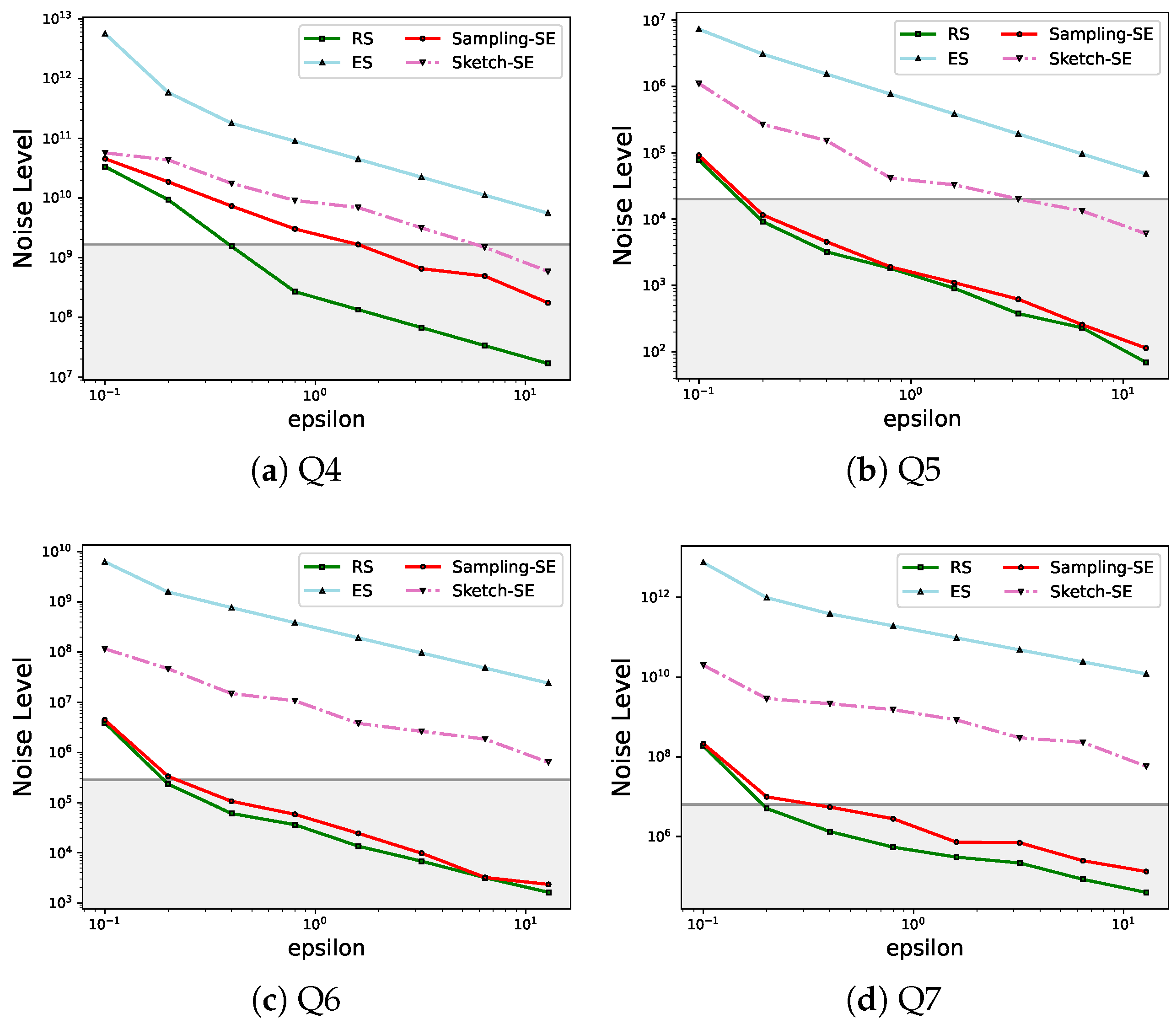
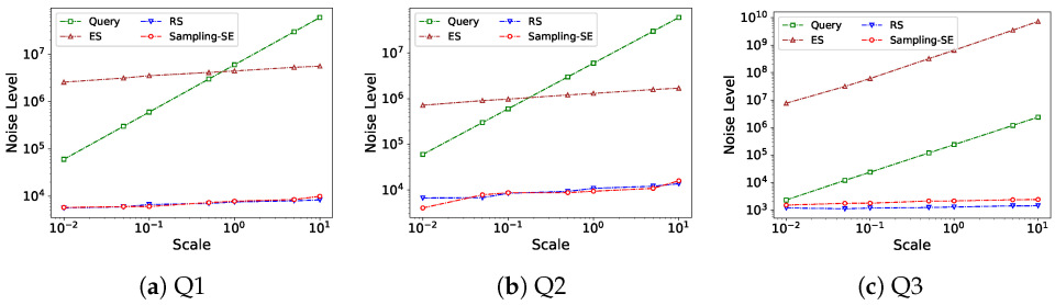
5.2. Accuracy

We evaluated the accuracy of our proposed Sampling-SE and Sketch-SE methods against ES and RS on the Facebook dataset, limiting the TPC-H comparison to Sampling-SE versus ES and RS due to the high cardinality of distinct values in TPC-H that makes sketch-based methods unsuitable for large-domain join results. We tested the noise level of different methods using $ϵ$ ranging from 0.1 to 12.8. The sampling rate was fixed at $1\times {10}^{-4}$ for Sampling-SE, and the number of estimators in each relation was set to 100,000 for Sketch-SE. The experimental results are shown in Figure 6 and Figure 7, respectively. The error is measured by the deviation from the true query result, i.e., the noise added. The shaded area indicates that the results have utility.

The results demonstrate that our Sampling-SE method achieves a noise level comparable to RS, with both significantly lower than ES, as shown in Figure 7. While Sketch-SE exhibits higher noise than Sampling-SE, it remains more accurate than ES. However, as query complexity increases (i.e., more relations and larger join-value domains), Sketch-SE requires substantially more estimators to maintain accuracy, making it less effective than Sampling-SE in such scenarios. This trade-off is further illustrated in Figure 7.

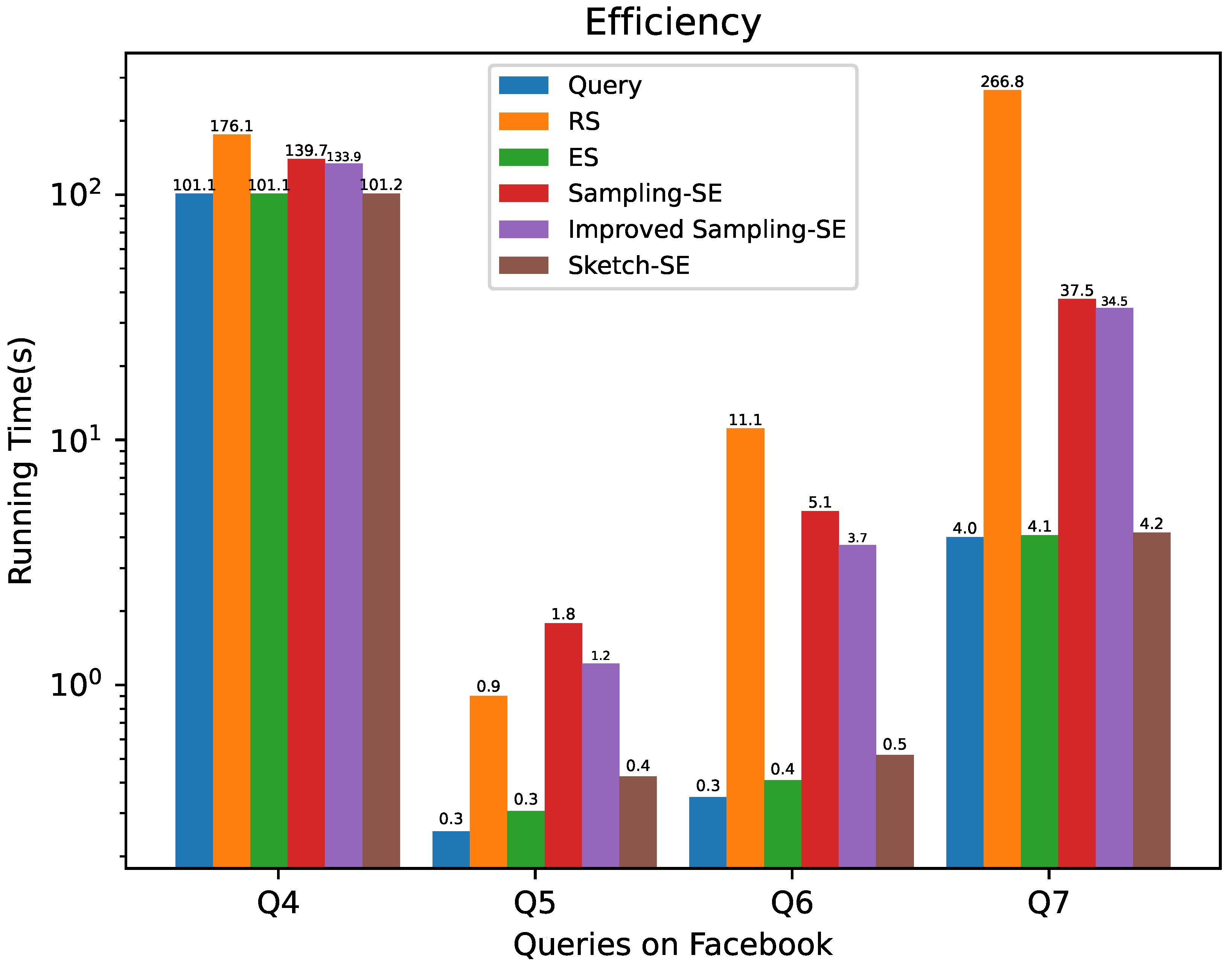
5.3. Efficiency

We evaluated the computational efficiency of our method against RS and ES by measuring end-to-end query processing time, from query submission to returning the noised results. This includes query execution time, sensitivity computation, and noise injection time under differential privacy. Note that the offline preprocessing steps (e.g., computing join attribute frequencies for ES or constructing relation sketches) are excluded from these measurements.

The experimental results on the TPC-H dataset in Figure 8 demonstrate that Sampling-SE consistently exhibits intermediate time efficiency between RS and ES, with the performance gap becoming particularly noticeable at larger scales. This behavior can be attributed to two key factors. First, the sampling approach significantly reduces the computational overhead of evaluating multiple residual queries. Second, certain complex residual queries involving primary-foreign key joins can be simplified to identifying the maximum frequency value within a single relation, yielding additional computational savings. This balanced efficiency–accuracy trade-off makes Sampling-SE particularly suitable for enterprise data warehouses that need to process large-scale, multi-relational queries under strict privacy constraints.

We also compared the efficiency of different methods on the Facebook dataset, and the results are plotted in Figure 9. We set the parameters $ϵ=0.8$ and $\delta ={10}^{-7}$ and the sample rate at $r=1\times {10}^{-4}$. The results demonstrate that Sampling-SE performs effectively in most scenarios. While slightly less efficient than RS for Q5, which involves only three small relations and, consequently, has minimal RS computation time, Sampling-SE shows superior scalability with larger datasets and complex join conditions, where its utility advantages become particularly significant. Notably, ES and Sketch-SE benefit from the offline pre-computation of statistics and sketches, respectively, giving them inherent online efficiency advantages over methods requiring real-time computation. This makes Sampling-SE ideal for real-world applications like fraud detection and customer profiling, which require both scalable join processing and rigorous privacy guarantees.

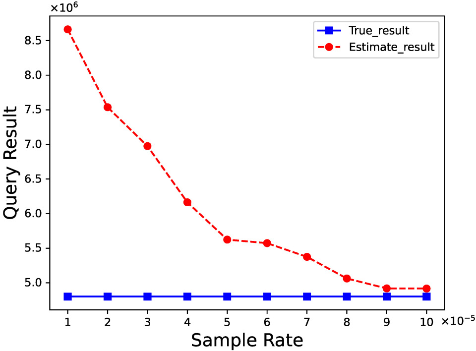
5.4. Impact of Parameters

Impact of Sample Size. The key factor of our Sampling-SE method is the sample rate. We conducted experiments to see how the sample rate r affects the noise results. For simplicity, we took two datasets and two chain queries (Q1 and Q4) for this experiment. For the parameters, we used the following: scale = 1 GB; $ϵ$ = 6.4; and $\delta =2\times {10}^{-10}$ for TPC-H, whereas we used $\delta ={10}^{-7}$ for the Facebook dataset. Moreover, different noise mechanisms, including the Laplace mechanism [8] and General Cauchy mechanism [9], were implemented to confirm our results. As shown in Figure 10, Sampling-SE significantly outperforms ES in accuracy across different differential privacy mechanisms. As sampling size increases, the noise level of Sampling-SE converges closer to the ground truth results. Furthermore, the Laplace mechanism consistently yields lower noise levels than the General Cauchy mechanism for all methods, including both baseline approaches and our proposed technique.

To further evaluate the efficacy of our sampling method, we examined a cyclic residual query, representing a key target scenario for Sampling-SE: “select max(count) from (select edge2_from, count(*) from $edge2\bowtie edge3\bowtie edge4\bowtie edge5$ group by edge2_from) as t;”. Figure 11 shows that even at low sampling rates, varying from ${10}^{-5}$ to ${10}^{-4}$, the method achieves highly accurate estimations. This confirms the effectiveness of Sampling-SE for complex cyclic queries while maintaining computational efficiency.

Additionally, we tested the effect of sampling rate on sensitivity as a way to eliminate the interference of the differential privacy noise added to the data. The experimental result is shown in Figure 12. To enhance efficiency for high-cardinality join results, we introduced Sampling-SE-WithFilter, a strategy that estimates only the maximum group size via random sampling rather than computing all group sizes. As illustrated, this approach achieves significantly faster convergence than basic Sampling-SE with increasing sampling rates.

Impact of Data scale. In this part, we evaluated the effects of data scale on the noise level. We used the TPC-H datasets with scale factors ranging from 0.01 to 10 and tested the performance of different methods with Q1, Q2, and Q3. We can see from Figure 13 that Sampling-SE maintains stable noise levels as data scales, confirming its suitability for large datasets. Note that for Q1 and Q2, Sampling-SE preserves the maximum boundaries of RS, yielding identical noise levels. To validate utility preservation, we compared noise magnitudes with the original query results. Crucially, Sampling-SE maintains noise levels strictly below the actual query answers, guaranteeing the original data insights remain clearly visible, which enables practical deployment in real-world applications where data utility is mission-critical.

5.5. Summary for Experimental Results

The experimental results are summarized as follows:

•

Sampling-SE and Sketch-SE both have higher efficiency than residual sensitivity for join queries with large-scale datasets;

•

With an appropriate sample rate, Sampling-SE has an equal level of accuracy to residual sensitivity while keeping a lower time overhead.

•

Sketch-SE has the same level of efficiency as elastic sensitivity but results in a relatively lower value of sensitivity, which leads to higher accuracy.

6. Discussion

These experimental findings demonstrate that our methods successfully address the fundamental efficiency–accuracy trade-off in differential privacy for join queries. The superior efficiency of Sampling-SE stems from its adaptive sampling strategy that focuses computational resources on high-impact residual queries, while the accuracy advantage of Sketch-SE originates from its ability to capture join attribute correlations through AGMS sketches. Notably, the maintained accuracy of Sampling-SE (compared to RS) and the improved accuracy of Sketch-SE (over ES) suggest that our approaches achieve better privacy–utility trade-offs without compromising their respective efficiency baselines. These results have important practical implications. For instance, Sampling-SE is suitable for skewed data due to minimizing sample waste on minor groups, and Sketch-SE enables real-time streaming protection through constant-time operation, which offers system designers flexible accuracy-latency trade-offs. The sampling-based and sketch-based sensitivity estimation methods proposed in this study significantly enhance the efficiency and accuracy of differential privacy protection for complex join queries. This breakthrough enables critical real-world applications, such as real-time anomaly detection in social networks, to achieve near non-private query utility while maintaining rigorous individual privacy protection with sub-second response times. By addressing the fundamental limitations of existing approaches, our work overcomes the key barriers to deploying large-scale privacy-preserving systems in practice. However, there are still some limitations that need to be considered. First, the sampling-based approach requires the careful tuning of sampling rates for optimal performance across different data distributions, which may increase implementation complexity. Second, the performance of our sketch-based approach may be impacted by data dimensionality and the number of join attributes, where high-dimensional join operations can amplify approximation errors due to the curse of dimensionality in sketch compression, and more join attributes require larger sketch sizes to maintain target accuracy levels. This paper establishes an effective framework for privacy-preserving query processing with immediate practical applications, while the limitations discussed provide promising directions for our future research.

7. Conclusions

In this paper, we present two novel approaches, Sampling-SE and Sketch-SE, for sensitivity estimation in differentially private multi-join queries. Sampling-SE achieves residual sensitivity-level accuracy while reducing computational overhead through adaptive random walks. Sketch-SE achieves higher accuracy than elastic sensitivity, with comparable efficiency via optimized AGMS sketches. These methods enable practical applications requiring both precision and speed, such as real-time social network analytics and large-scale medical data linkage, while establishing theoretical guarantees for complex query classes. Future work will explore extensions to more complex query types, including those with advanced predicates and user-defined functions, further broadening the applicability of these techniques.

References

- Tabassum, S.; Pereira, F.S.; Fernandes, S.; Gama, J. Social network analysis: An overview. Wiley Interdiscip. Rev. Data Min. Knowl. Discov. 2018, 8, e1256. [Google Scholar] [CrossRef]
- Singh, S.S.; Muhuri, S.; Mishra, S.; Srivastava, D.; Shakya, H.K.; Kumar, N. Social network analysis: A survey on process, tools, and application. ACM Comput. Surv. 2024, 56, 1–39. [Google Scholar] [CrossRef]
- Chen, C.M.; Agrawal, H.; Cochinwala, M.; Rosenbluth, D. Stream query processing for healthcare bio-sensor applications. In Proceedings of the IEEE 20th International Conference on Data Engineering, Boston, MA, USA, 30 March–2 April 2004; pp. 791–794. [Google Scholar]
- Soni, K.; Sachdeva, S.; Minj, A. Querying Healthcare Data in Knowledge-Based Systems. In Proceedings of the International Conference on Big Data Analytics, Sorrento, Italy, 15–18 December 2023; Springer: Berlin/Heidelberg, Germany, 2023; pp. 59–77. [Google Scholar]
- Bell, R.M.; Koren, Y. Lessons from the Netflix prize challenge. ACM Sigkdd Explor. Newsl. 2007, 9, 75–79. [Google Scholar] [CrossRef]
- Barbaro, M.; Zeller, T.; Hansell, S. A face is exposed for AOL searcher no. 4417749. New York Times 2006, 9, 8. [Google Scholar]
- Dwork, C. Differential Privacy. In Proceedings of the Encyclopedia of Cryptography and Security; Springer: Berlin/Heidelberg, Germany, 2006. [Google Scholar]
- Dwork, C.; McSherry, F.; Nissim, K.; Smith, A.D. Calibrating Noise to Sensitivity in Private Data Analysis. In Proceedings of the Theory of Cryptography Conference, New York, NY, USA, 4–7 March 2006. [Google Scholar]
- Nissim, K.; Raskhodnikova, S.; Smith, A.D. Smooth sensitivity and sampling in private data analysis. In Proceedings of the Symposium on the Theory of Computing, San Diego, CA, USA, 11–13 June 2007. [Google Scholar]
- Johnson, N.M.; Near, J.P.; Song, D.X. Towards Practical Differential Privacy for SQL Queries. Proc. VLDB Endow. 2017, 11, 526–539. [Google Scholar] [CrossRef]
- Dong, W.; Yi, K. Residual Sensitivity for Differentially Private Multi-Way Joins. In Proceedings of the 2021 International Conference on Management of Data, Xi’an, China, 20–25 June 2021. [Google Scholar]
- Dobra, A.; Garofalakis, M.N.; Gehrke, J.; Rastogi, R. Processing complex aggregate queries over data streams. In Proceedings of the Proceedings of the 2002 ACM SIGMOD International Conference on Management of Data, Madison, WI, USA, 3–6 June 2002; Franklin, M.J., Moon, B., Ailamaki, A., Eds.; ACM: New York, NY, USA, 2002; pp. 61–72. [Google Scholar] [CrossRef]
- Aydöre, S.; Brown, W.; Kearns, M.; Kenthapadi, K.; Melis, L.; Roth, A.; Siva, A. Differentially Private Query Release Through Adaptive Projection. In Proceedings of the International Conference on Machine Learning, Virtual, 18–24 July 2021. [Google Scholar]
- Wang, T.; Chen, J.Q.; Zhang, Z.; Su, D.; Cheng, Y.; Li, Z.; Li, N.; Jha, S. Continuous Release of Data Streams under both Centralized and Local Differential Privacy. In Proceedings of the 2021 ACM SIGSAC Conference on Computer and Communications Security, Virtual Event, Republic of Korea, 15–19 November 2021. [Google Scholar]
- Maruseac, M.; Ghinita, G. Precision-Enhanced Differentially-Private Mining of High-Confidence Association Rules. IEEE Trans. Dependable Secur. Comput. 2020, 17, 1297–1309. [Google Scholar] [CrossRef]
- Wang, T.; Li, N.; Jha, S. Locally Differentially Private Frequent Itemset Mining. In Proceedings of the 2018 IEEE Symposium on Security and Privacy (SP), San Francisco, CA, USA, 21–23 May 2018; pp. 127–143. [Google Scholar]
- Triastcyn, A.; Faltings, B. Bayesian Differential Privacy for Machine Learning. In Proceedings of the International Conference on Machine Learning, Long Beach, CA, USA, 9–15 June 2019. [Google Scholar]
- Zheng, H.; Ye, Q.; Hu, H.; Fang, C.; Shi, J. Protecting Decision Boundary of Machine Learning Model With Differentially Private Perturbation. IEEE Trans. Dependable Secur. Comput. 2020, 19, 2007–2022. [Google Scholar] [CrossRef]
- Jiang, H.; Pei, J.; Yu, D.; Yu, J.; Gong, B.; Cheng, X. Applications of Differential Privacy in Social Network Analysis: A Survey. IEEE Trans. Knowl. Data Eng. 2023, 35, 108–127. [Google Scholar] [CrossRef]
- Erlingsson, Ú.; Pihur, V.; Korolova, A. Rappor: Randomized aggregatable privacy-preserving ordinal response. In Proceedings of the 2014 ACM SIGSAC Conference on Computer and Communications Security, Scottsdale, AZ, USA, 3–7 November 2014; pp. 1054–1067. [Google Scholar]
- Ding, B.; Kulkarni, J.; Yekhanin, S. Collecting telemetry data privately. Adv. Neural Inf. Process. Syst. 2017, 30, 3571–3580. [Google Scholar]
- McSherry, F. Privacy integrated queries: An extensible platform for privacy-preserving data analysis. In Proceedings of the 2009 ACM SIGMOD International Conference on Management of Data, Providence, RI, USA, 29 June–2 July 2009. [Google Scholar]
- Proserpio, D.; Goldberg, S.; McSherry, F. Calibrating Data to Sensitivity in Private Data Analysis. Proc. VLDB Endow. 2012, 7, 637–648. [Google Scholar] [CrossRef]
- Chaudhuri, S.; Ding, B.; Kandula, S. Approximate Query Processing: No Silver Bullet. In Proceedings of the 2017 ACM International Conference on Management of Data, Chicago, IL, USA, 14–19 May 2017. [Google Scholar]
- Ganguly, S.; Gibbons, P.B.; Matias, Y.; Silberschatz, A. Bifocal sampling for skew-resistant join size estimation. In Proceedings of the 1996 ACM SIGMOD International Conference on Management of Data, Montreal, QC, Canada, 4–6 June 1996; pp. 271–281. [Google Scholar]
- Estan, C.; Naughton, J.F. End-biased samples for join cardinality estimation. In Proceedings of the IEEE 22nd International Conference on Data Engineering (ICDE’06), Atlanta, GA, USA, 3–7 April 2006; p. 20. [Google Scholar]
- Haas, P.J.; Hellerstein, J.M. Ripple joins for online aggregation. In Proceedings of the ACM SIGMOD Conference, Philadelphia, PA, USA, 1–3 June 1999. [Google Scholar]
- Li, F.; Wu, B.; Yi, K.; Zhao, Z. Wander Join: Online Aggregation via Random Walks. In Proceedings of the 2016 International Conference on Management of Data, San Francisco, CA, USA, 26 June–1 July 2016. [Google Scholar] [CrossRef]
- Zhao, Z.; Christensen, R.; Li, F.; Hu, X.; Yi, K. Random Sampling over Joins Revisited. In Proceedings of the 2018 International Conference on Management of Data, Houston, TX, USA, 10–15 June 2018. [Google Scholar]
- Ioannidis, Y.E.; Christodoulakis, S. Optimal histograms for limiting worst-case error propagation in the size of join results. ACM Trans. Database Syst. (TODS) 1993, 18, 709–748. [Google Scholar] [CrossRef]
- Ioannidis, Y.E.; Poosala, V. Balancing histogram optimality and practicality for query result size estimation. ACM Sigmod Rec. 1995, 24, 233–244. [Google Scholar] [CrossRef]
- Bater, J.; Park, Y.; He, X.; Wang, X.; Rogers, J. Saqe: Practical privacy-preserving approximate query processing for data federations. Proc. VLDB Endow. 2020, 13, 2691–2705. [Google Scholar] [CrossRef]
- Ock, J.; Lee, T.; Kim, S. Privacy-preserving approximate query processing with differentially private generative models. In Proceedings of the 2023 IEEE International Conference on Big Data (BigData), Sorrento, Italy, 15–18 December 2023; pp. 6242–6244. [Google Scholar]
- Alon, N.; Gibbons, P.B.; Matias, Y.; Szegedy, M. Tracking join and self-join sizes in limited storage. In Proceedings of the Eighteenth ACM SIGMOD-SIGACT-SIGART Symposium on Principles of Database Systems, Philadelphia, PA, USA, 31 May–2 June 1999; pp. 10–20. [Google Scholar]
- Charikar, M.; Chen, K.; Farach-Colton, M. Finding frequent items in data streams. In Proceedings of the International Colloquium on Automata, Languages, and Programming, Malaga, Spain, 8–13 July 2002; Springer: Berlin/Heidelberg, Germany, 2002; pp. 693–703. [Google Scholar]
- Cormode, G.; Muthukrishnan, S. An improved data stream summary: The count-min sketch and its applications. J. Algorithms 2005, 55, 58–75. [Google Scholar] [CrossRef]
- Vengerov, D.; Menck, A.C.; Zaït, M.; Chakkappen, S. Join Size Estimation Subject to Filter Conditions. Proc. VLDB Endow. 2015, 8, 1530–1541. [Google Scholar] [CrossRef]
- Zhang, M.; Liu, X.; Yin, L. Sketches-based join size estimation under local differential privacy. In Proceedings of the 2024 IEEE 40th International Conference on Data Engineering (ICDE), Utrecht, The Netherlands, 13–16 May 2024; pp. 1726–1738. [Google Scholar]
- Cormode, G.; Garofalakis, M. Sketching streams through the net: Distributed approximate query tracking. In Proceedings of the 31st International Conference on Very Large Data Bases, Trondheim, Norway, 30 August–2 September 2005; pp. 13–24. [Google Scholar]
- Kim, A.; Blais, E.; Parameswaran, A.G.; Indyk, P.; Madden, S.; Rubinfeld, R. Rapid Sampling for Visualizations with Ordering Guarantees. Proc. VLDB Endow. 2015, 8, 521–532. [Google Scholar] [CrossRef] [PubMed]
- Hoeffding, W. Probability Inequalities for Sums of Bounded Random Variables. J. Am. Stat. Assoc. 1963, 58, 13. [Google Scholar] [CrossRef]
- Rusu, F.; Dobra, A. Sketches for size of join estimation. ACM Trans. Database Syst. (TODS) 2008, 33, 1–46. [Google Scholar] [CrossRef]
Disclaimer/Publisher’s Note: The statements, opinions and data contained in all publications are solely those of the individual author(s) and contributor(s) and not of MDPI and/or the editor(s). MDPI and/or the editor(s) disclaim responsibility for any injury to people or property resulting from any ideas, methods, instructions or products referred to in the content. |
© 2025 by the authors. Licensee MDPI, Basel, Switzerland. This article is an open access article distributed under the terms and conditions of the Creative Commons Attribution (CC BY) license (https://creativecommons.org/licenses/by/4.0/).
Share and Cite
Zhang, M.; Liu, X.; Yin, L. Sensitivity Estimation for Differentially Private Query Processing. Appl. Sci. 2025, 15, 7667. https://doi.org/10.3390/app15147667
Zhang M, Liu X, Yin L. Sensitivity Estimation for Differentially Private Query Processing. Applied Sciences. 2025; 15(14):7667. https://doi.org/10.3390/app15147667
Chicago/Turabian StyleZhang, Meifan, Xin Liu, and Lihua Yin. 2025. "Sensitivity Estimation for Differentially Private Query Processing" Applied Sciences 15, no. 14: 7667. https://doi.org/10.3390/app15147667
APA StyleZhang, M., Liu, X., & Yin, L. (2025). Sensitivity Estimation for Differentially Private Query Processing. Applied Sciences, 15(14), 7667. https://doi.org/10.3390/app15147667