Discrete Element Simulation Parameter Calibration of Wheat Straw Feed Using Response Surface Methodology and Particle Swarm Optimization–Backpropagation Hybrid Algorithm

Abstract

To establish a fundamental property database for discrete elements targeting long-fiber materials and address the issue of response surface methodology (RSM) being prone to local optima in high-dimensional nonlinear optimization, this study conducted parameter calibration experiments and validated the calibrated parameters through a combined approach of simulation and physical testing. The Plackett–Burman design and steepest ascent test were employed to screen significant factors. Using the angle of repose (42.3°) obtained from physical experiments as the response value, response surface methodology (RSM) and a particle swarm optimization–back propagation (PSO-BP) neural network model were independently applied to optimize and compare the critical parameters. The results demonstrated that the dynamic friction coefficient between wheat straw particles, the static friction coefficient between wheat straw and steel plate, and the JKR surface energy were the most influential factors on the simulated angle of repose. The PSO-BP model exhibited superior optimization performance compared to RSM, yielding an optimal parameter combination of 0.17, 0.46, and 0.03. The simulated repose angle under these conditions was 41.67°, exhibiting a relative error of only 1.5% compared to the physical experiment. These findings provide a robust theoretical foundation for discrete element simulations of wheat straw feedstock.

1. Introduction

Since the initiation of China’s 14th Five-Year Plan period, the livestock industry has emerged as a pivotal pillar of the agricultural economy, with sustainable development playing a critical role in advancing modern animal husbandry [1]. China possesses abundant wheat straw resources, with an annual output of approximately 700–800 million tons, accounting for 30% of the global total. Rice straw, corn straw, and wheat straw collectively constitute 80% of the national straw yield, with wheat straw alone contributing nearly one-fourth (1.9 billion tons) [2]. Wheat straw feedstock is nutritionally rich, containing substantial trace elements, and serves as a versatile, renewable bioresource, making it a vital raw material for ruminant feeding systems such as cattle and sheep [3]. Currently, China’s livestock sector is undergoing transformative development, prioritizing intensification and scale efficiency while advancing mechanization, digitalization, and standardization [4]. Wheat straw forage, as an important roughage resource, involves complex granular mechanics behaviors during processes like forage utilization, silage production, and compaction forming, requiring precise simulation to support equipment design optimization. Existing calibration methods lack sufficient applicability for long-fiber materials like wheat straw. The core objective of this study is to establish a set of high-precision, high-efficiency parameter calibration methods for wheat straw forage.

The discrete element method (DEM), which tracks the microscopic motion of individual particles to reveal the macroscopic mechanical behavior of granular systems, has been widely applied in agricultural engineering due to its time- and labor-efficient nature, cost-effectiveness, and visualization capabilities. Researchers globally have conducted discrete element modeling and parameter calibration for materials such as soils and grains; Zhao et al. calibrated the contact parameters between substrate particles based on the Hertz–Mindlin with the JKR cohesion contact model through integrated repose angle simulation tests, optimized the dominant parameters using the response surface methodology, and obtained the simulated repose angle at the optimal solution; the validity of the calibrated parameters was verified via rotary tillage tests [5]. Sun et al. calibrated the contact parameters between soil particles on loess plateau slopes using the same method as Zhao et al., and also obtained the simulated repose angle at the optimal solution; the validity of the calibrated parameters was verified through slope rotary tillage tests on the loess plateau [6]. Du et al. established a discrete element model of Capsicum annuum based on reverse engineering, calibrated and optimized its contact parameters using the response surface methodology, and determined the repose angle via the cylinder-lifting method; the validity of the calibrated parameters was demonstrated [7]. Li et al. took corncobs as the research object, calibrated their contact parameters using Plackett–Burman and Box–Behnken experiments, determined the optimal parameter combination through the response surface methodology, and verified the accuracy of the calibrated parameters via corncob bending simulation tests [8].

The results indicate that all aforementioned studies employed response surface methodology (RSM) to optimize significant parameters. RSM typically uses second-order polynomials (e.g., quadratic regression models) to fit response surfaces, which tends to trap in local optima and exhibits limited capability for high-dimensional nonlinearity. Consequently, it struggles to address complex nonlinear optimization problems in DEM parameter calibration. Moreover, parameter optimization for wheat straw forage presents specific challenges: the contact mechanics of long-fiber materials inherently involve strong nonlinearity, with notable rolling friction and bonding effects, making them far more complex than spherical particles. Reportedly, existing RSM methods achieve a maximum relative error of 15.17% for similar materials [9], highlighting an urgent need for resolution.

Machine learning can address such issues. As a novel nonlinear regression modeling technique, it demonstrates significant model adaptability and high-precision prediction advantages when handling multidimensional data fitting, complex system prediction, and global optimization problems. Specifically, the particle swarm optimization–backpropagation (PSO-BP) neural network achieves collaborative optimization of network parameters by introducing swarm intelligence optimization mechanisms. This approach avoids the tendency of response surface methodology (RSM) to settle for local optima, making it more suitable for attaining globally optimal combinatorial design objectives with superior fitting accuracy and precise predictive capabilities. Wang et al. developed a PSO-BP neural network model to predict moisture content during the drying process of impregnated bamboo bundles. By optimizing initial weights and thresholds of the BP neural network using the PSO algorithm, they mitigated RSM’s susceptibility to local optima. Physical validation through full factorial experimental design confirmed the feasibility and effectiveness of the PSO-BP neural network model’s predictive ability [10]. Thus, this study aims to construct a PSO-BP model to establish a high-precision, high-efficiency parameter calibration method for wheat straw forage.

This study will design the parameter sample space using key significant parameters screened by RSM, construct a PSO-BP surrogate model based on datasets generated through EDEM simulations, and train, validate, and predict this network to optimize a feasible and effective neural network prediction model. The globally optimized parameter combination will be obtained, and results will be comparatively analyzed with physical repose angle tests, aiming to avoid the tendency of RSM to produce local optima. An intelligent discrete element calibration framework for wheat straw long-fiber structures will be established, providing a paradigm for parameter calibration of materials such as straw and forage.

2. Materials and Methods

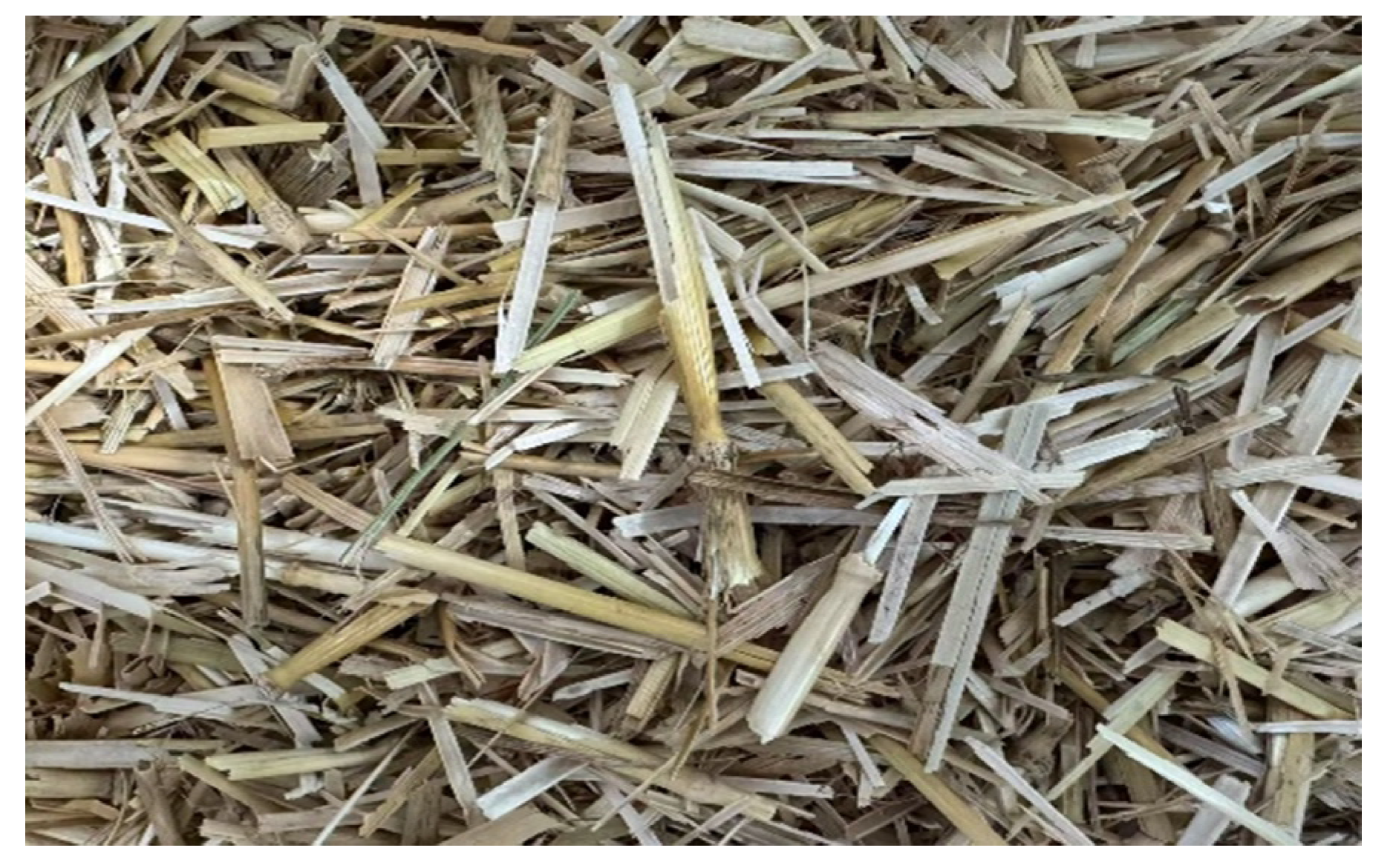
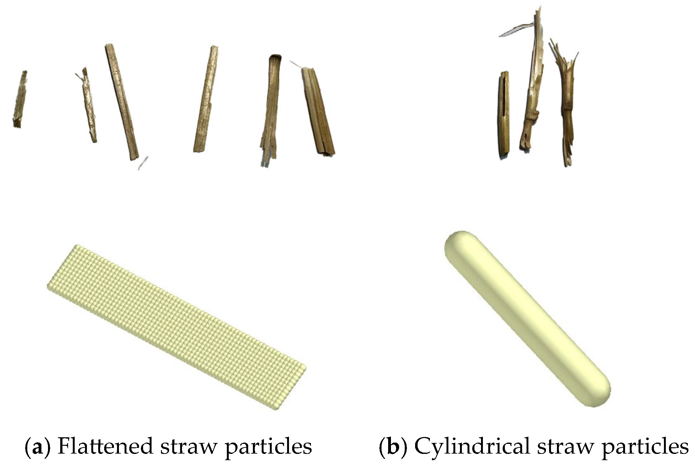
2.1. Test Samples

The wheat straw feedstock used in this study was derived from the D1508 cultivar, cultivated in Changji City, Xinjiang Uygur Autonomous Region (elevation: 617 m). Post-harvest, the straw was processed using an MF1840 straw shredding and collection machine to achieve uniform fragmentation. The shredded material was subsequently stored at the Animal Husbandry Experimental Field Station of the Xinjiang Academy of Agricultural Sciences (Anningqu Town, Changji, China) under controlled environmental conditions to preserve its physicochemical properties for downstream experiments. As illustrated in Figure 1, the processed wheat straw feed exhibited a loose, fragmented structure with high morphological consistency.

Key physical parameters, including particle geometry (external dimensions), moisture content, and bulk density, were experimentally quantified. To facilitate DEM calibration, additional mechanical properties—such as the coefficient of friction (inter-particle and particle-steel plate), shear modulus, and Poisson’s ratio—were characterized using standardized tribological and rheological testing protocols. These measurements ensured the input parameters for the DEM simulations aligned with the intrinsic behavior of the wheat straw feedstock under operational conditions.

2.2. Characterization of Material Properties

2.2.1. Geometric Properties

Wheat straw feedstock samples were randomly collected at the Animal Husbandry Experimental Field Station and subjected to sieving and characterization using a sieving machine equipped with standardized sieves, an electronic balance, vernier calipers, and auxiliary instruments. Ten parallel measurements were conducted simultaneously to determine particle size distribution, mass, and morphological properties, with results detailed in

Table 1. Size and mass distribution of wheat straw feedstock.

Sieve Fraction	Upper Sieve	Middle Sieve	Lower Sieve
Size range (mm)	>40	20 ≤ particle size ≤ 40	<20
Mean size (mm)	45	26	9
Mass percentage (%)	18.07%	45.22%	36.71%
Hollow straws (proportion)	1/3	1/4	0
Flattened straws (proportion)	2/3	3/4	1

.

2.2.2. Moisture Content

Moisture content was determined according to the Chinese National Standard GB/T 6435-2014 [11,12]. The experimental procedure comprised the following steps:

• Sample Preparation:
  The feedstock was ground into homogeneous particles (passed through a 40-mesh sieve) and thoroughly mixed to minimize hygroscopic or dehydrative effects during handling.
• Weighing:
  A pre-dried weighing dish (with lid) was tared and recorded (W1). Subsequently, 2–5 g of sample was added and precisely weighed to 0.0001 g (W2) using a BSA3202S electronic analytical balance.
• Drying:
  The uncovered dish was placed in a preheated oven (Model 101 Electric Blast Drying Oven) at 105 °C for 4 h. After drying, the dish was immediately sealed and transferred to a desiccator for cooling to room temperature (~30 min).
• Constant Mass Verification:
  The cooled sample was reweighed (W3).
  The drying–cooling–weighing cycle was repeated at 1 h intervals until successive weight differences were ≤0.05%.
• Calculation:
  Moisture content (MC) was calculated as

$$MC\%={\displaystyle \frac{W_2-W_3}{W_2-W_1}}\times 100,$$

(1)

6.

Final Moisture Content

Ten parallel trials were conducted, with results summarized in

Table 2. Moisture content of wheat straw feedstock.

Sample No	1	2	3	4	5	6	7	8	9	10
Moisture Content (%)	12.42	11.57	11.85	11.93	12.73	11.03	10.83	11.52	10.83	11.21

. The final moisture content of the wheat straw feedstock was determined to be 11.59%.

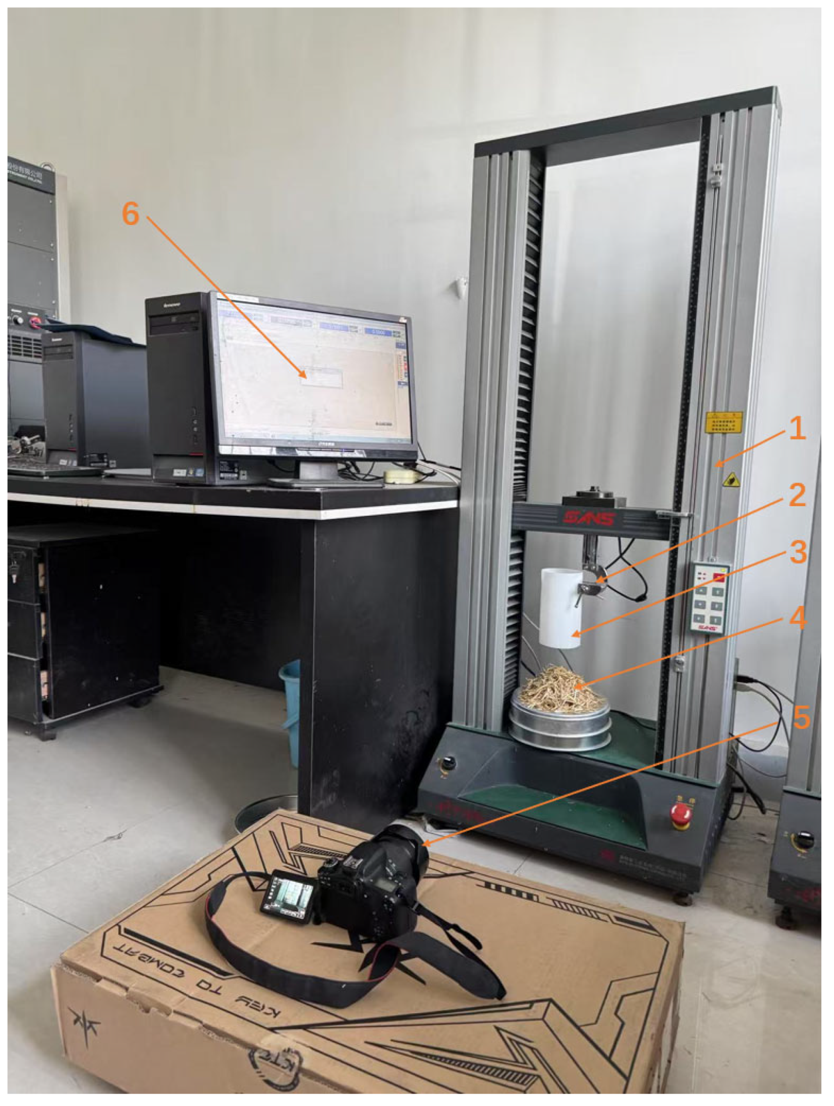
2.2.3. Bulk Density Determination

Bulk density determination was conducted in accordance with the Chinese Agricultural Standard NY/T 1881.6-2010 [13], following the procedure below [14].

• Sample Preparation:

Representative samples of wheat straw feedstock were randomly collected and prepared at the Animal Husbandry Experimental Field Station under standardized protocols.

2.

Container Filling:

The sample was freely poured into a calibrated standard container, and the surface was leveled using a straight-edge scraper. The total mass (m₁) was then recorded.

3.

Weighing and Calculation:

The empty container mass (m₂) was measured prior to filling.

Bulk density (ρ) was calculated as:

$$\mathsf{\rho }={\displaystyle \frac{m_1-m_2}{V_{container}}},$$

(2)

4.

Finalized Bulk Density

Ten parallel trials were performed, with results detailed in

Table 3. Density of wheat straw feedstock.

Sample No	1	2	3	4	5	6	7	8	9	10
Density (kg/m3)	45.18	45.72	47.40	44.77	45.17	46.32	45.38	46.55	45.85	11.21

. The bulk density of the wheat straw feedstock was determined to be 45.82 kg/m³.

2.2.4. Determination of Friction Coefficients

The static friction coefficient measurement setup is illustrated in Figure 2. To determine the static friction coefficient between the material and steel plate, the test sample was placed on the steel plate and lightly compacted to ensure full contact. The plate was initially positioned at 0°, and then gradually inclined until the onset of sliding motion. The tilt angle (θ) at this threshold was recorded. Ten replicate trials were conducted, and the average value was calculated. The static friction coefficient (μ) was derived using the following formula:

$$\mu =tan\theta ,$$

(3)

where

μ: Coefficient of friction (dimensionless);

θ: Tilt angle of the inclined plane apparatus (°).

To determine the static friction coefficient between wheat straw feedstock particles, the material was evenly spread and adhered to a steel plate, forming a cohesive wheat straw layer. The aforementioned tilt table test was repeated, and the critical inclination angle (θ)was recorded. Using Equation (3), the static friction coefficients were calculated as 0.52 (straw–straw) and 0.47 (straw–steel).

Figure 2. Home-made inclined plane instrument.

Figure 2. Home-made inclined plane instrument.

The rolling friction coefficient was determined using the same instrumentation and methodology as described for static friction measurements. The inclination angle at the onset of rolling motion was recorded using the tilt table apparatus, with ten replicate trials conducted to calculate the mean value. Applying Equation (3), the rolling friction coefficients between wheat straw feedstock particles (straw–straw) and between wheat straw and steel (straw–steel) were determined to be 0.18 and 0.19, respectively.

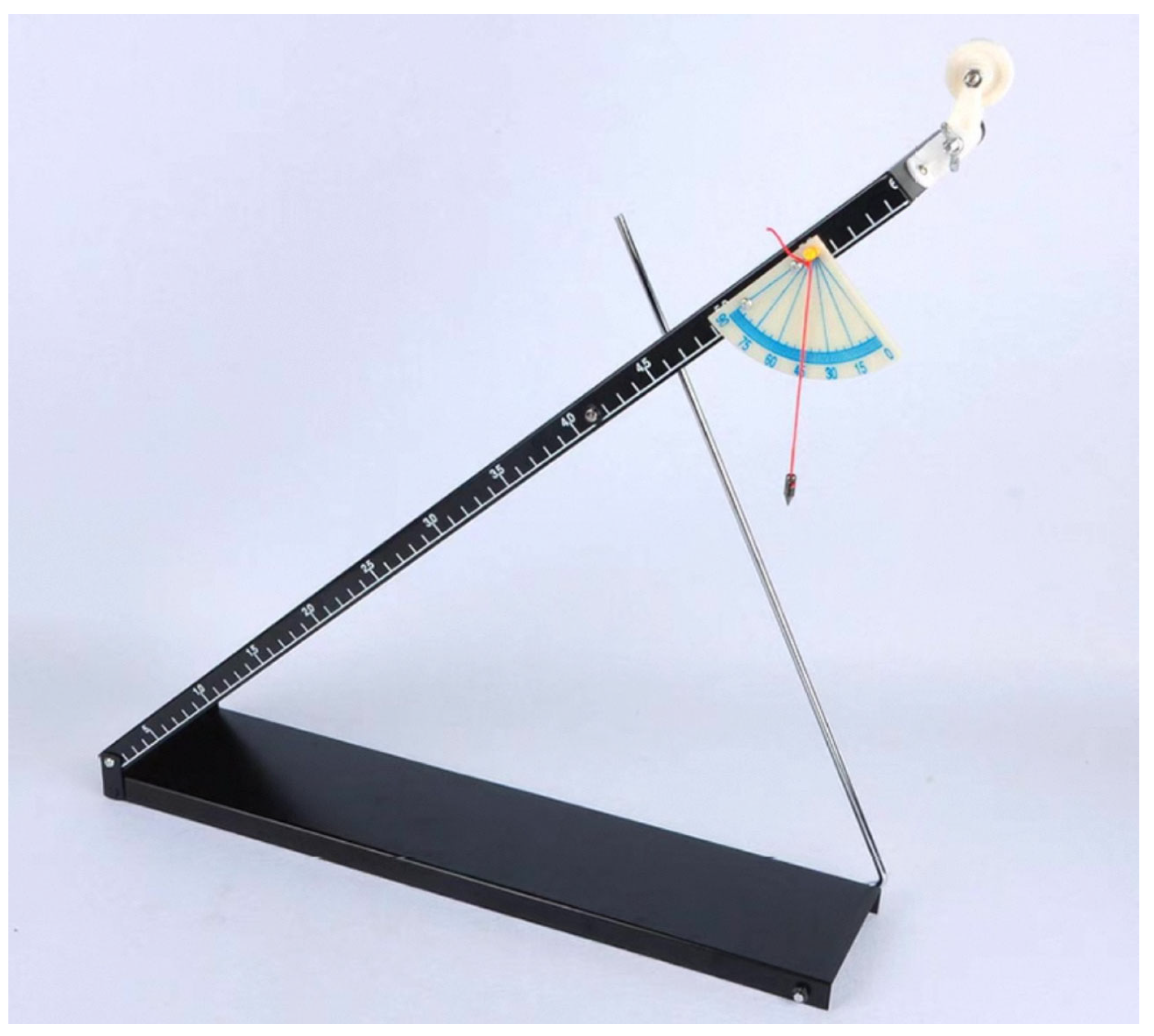
2.2.5. Determination of Restitution Coefficient

The coefficients of restitution (COR) between wheat straw particles and between wheat straw and steel plates were determined using a free-fall impact test, with the experimental setup illustrated in Figure 3 [15]. A wheat straw specimen plate or steel plate was selected as the impact surface. Wheat straw particles were released from a height of 250 mm above the impact plate, and a high-speed camera recorded the rebound trajectories to measure the rebound height (H2). Ten replicate trials were conducted for each material pairing, and the mean values were calculated. The coefficient of restitution (e) was derived using the following formula:

$$e={\displaystyle \frac{v_y}{v}}={\displaystyle \frac{\sqrt{2g{H}_1}}{\sqrt{2g{H}_2}}}=\sqrt{{\displaystyle \frac{H_1}{H_2}}},$$

(4)

where

e: Coefficient of restitution (dimensionless);

v_y: Post-impact normal velocity (mm/s);

v: Post-impact velocity (mm/s);

H₁: Initial free-fall height (mm);

H₂: Rebound height after collision with the impact plate (mm).

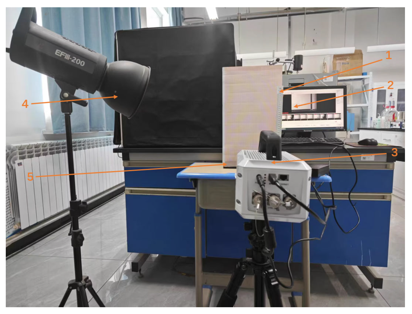
2.2.6. Determination of the Angle of Repose

The repose angle was measured using a cylindrical lift apparatus (Figure 4) [16]. The experimental setup involved loading wheat straw feed into a steel cylinder (inner diameter: 90 mm; height: 180 mm), which was vertically lifted by a CMT-6103 microcomputer-controlled electronic universal testing machine at a constant velocity of 0.6 m/s. This lifting speed, optimized through preliminary trials, ensured stable formation of the material pile on a horizontal baseplate.

High-resolution vertical images of the pile were captured for subsequent processing in MATLAB R2022b. The workflow included the following:

• Grayscale Conversion: Raw images (Figure 5a) were converted to grayscale (Figure 5b) to enhance contrast.
• Binarization: An iterative threshold segmentation algorithm was applied to generate binary images (Figure 5c), isolating the pile from the background.
• Boundary Extraction: The bwperim function detected the pile perimeter, followed by morphological filling (imfill function) to eliminate internal noise and obtain a continuous closed boundary (Figure 5d).
• Slope Calculation: Boundary coordinates extracted using Origin’s Digitizer tool were linearly fitted, and the repose angle was derived from the slope of the fitted line.

This method achieved high precision in quantifying the repose angle, with results validated against physical measurements, ensuring robustness for DEM parameter calibration.

2.3. Establishment of Material Simulation Models

2.3.1. Creation of Particle and Experimental Setup Models

The discrete element method (DEM) was employed to model wheat straw feed particles, with geometric characteristics derived from Table 1 informing the design of two distinct particle types: flattened straw and cylindrical straw [17]. The flattened straw particles were constructed using a multi-sphere superposition method, while cylindrical straw particles were modeled as rod-shaped geometries (Figure 6). Particle size distributions were standardized to the mean values of each sieve fraction to ensure mass consistency and simulation fidelity.

A three-dimensional steel cylinder model, designed in SolidWorks 2022, was imported into EDEM 2023 to replicate the experimental apparatus. Material properties for the steel substrate were assigned in accordance with reference [18]: Poisson’s ratio = 0.3, density = 7850 kg/m³, and shear modulus = 75 GPa. These parameters ensured accurate representation of particle–substrate interactions during DEM simulations.

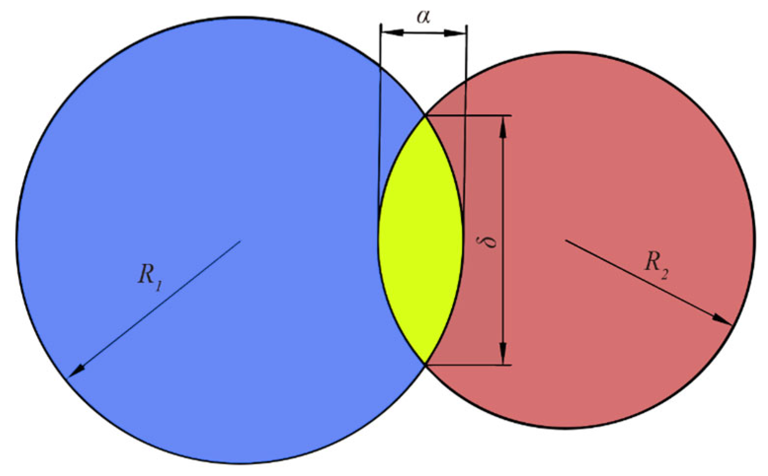
2.3.2. Contact Model Setup

Given the presence of wheat straw particles with diameters below 9 mm in the material, cohesive interactions between particles were anticipated due to electrostatic and surface energy effects. To account for these agglomeration phenomena, the Hertz–Mindlin with JKR (Johnson–Kendall–Roberts) cohesion contact model was selected for DEM parameter calibration [19]. This model, rooted in Hertzian contact theory, explicitly incorporates cohesive forces, making it particularly suitable for simulating materials prone to particle bonding and clustering (Figure 7).

In the JKR cohesion simplified framework, the normal elastic force effectively characterizes the viscoelastic behavior between particles. This force is governed by the normal overlap and surface energy, ensuring accurate representation of adhesion dynamics. The model’s ability to balance elastic recovery and energy dissipation during particle collisions aligns with the observed agglomerative tendencies of fine wheat straw particles, thereby enhancing simulation fidelity for biomass systems with inherent cohesive properties.

$$F_{JKR}=-4\sqrt{\mathsf{\pi }\mathsf{\gamma }{E}^{*}}{\mathsf{\alpha }}^{{\displaystyle \frac{3}{2}}}+{\displaystyle \frac{4E^{*}}{3R^{*}}}{\mathsf{\alpha }}^3,$$

(5)

$$\mathsf{\delta }={\displaystyle \frac{{\mathsf{\alpha }}^2}{R^{*}}}-\sqrt{{\displaystyle \frac{4\mathsf{\pi }\mathsf{\gamma }\mathsf{\alpha }}{E^{*}}}},$$

(6)

$$\frac{1}{E^{*}}=\frac{1-U_1^2}{E_1}+\frac{1-U_2^2}{E_2},$$

(7)

$${\displaystyle \frac{1}{R^{*}}}={\displaystyle \frac{1}{R_1}}+{\displaystyle \frac{1}{R_2}},$$

(8)

where

F_JKR: JKR normal elastic force (N);

α: Normal overlap between contacting particles (m);

δ: Tangential overlap between contacting particles (m);

γ: Surface energy (J/m²);

E*: Effective elastic modulus (Pa);

R*: Effective contact radius (m);

E₁, E₂: Elastic modulus of contacting particles (Pa);

U₁, U₂: Poisson’s ratio of contacting particles (dimensionless);

R₁, R₂: Contact radius between particles (m).

When the surface energy γ = 0, the JKR normal elastic force reduces to the Hertz–Mindlin normal force, expressed as

$$F_{JKR}=F_{Hertz}=\frac{4}{3}{E}^{*}\sqrt{R^{*}{\mathsf{\delta }}^{\frac{3}{2}}},$$

(9)

Even when particles are not in direct contact, the JKR contact model accounts for attractive cohesive forces. The maximum normal (α_c) and tangential (δ_c) gaps for cohesive interactions between particles are defined as

$${\mathsf{\alpha }}_c={\left[{\displaystyle \frac{9\mathsf{\pi }\mathsf{\gamma }{R^{*}}^2}{2E^{*}}}-\left({\displaystyle \frac{3}{4}}-{\displaystyle \frac{1}{\sqrt{2}}}\right)\right]}^{{\displaystyle \frac{1}{3}}},$$

(10)

$${\mathsf{\delta }}_c={\displaystyle \frac{{\mathsf{\alpha }}_c^2}{R^{*}}}-\sqrt{{\displaystyle \frac{4{\mathsf{\pi }\mathsf{\gamma }\mathsf{\alpha }}_c}{E^{*}}}},$$

(11)

where

α_c: Normal maximum gap between particles under non-zero cohesive forces (m);

δ_c: Tangential maximum gap between particles under non-zero cohesive forces (m).

When particles are not in direct contact and their separation is less than δc, the JKR cohesive force reaches its maximum value, given by

$$F_{\mathrm{pull}\text{-}\mathrm{out}}=-{\displaystyle \frac{3}{2}}\mathsf{\pi }\mathsf{\gamma }{R}^{*},$$

(12)

2.3.3. Selection of Simulation Parameters

The discrete element method (DEM) simulation parameters for wheat straw feedstock and steel plate were determined by integrating experimental measurements with established methodologies from existing literature [20]. Key parameters, including material properties and interaction coefficients, are summarized in

Table 4. DEM simulation parameters for the repose angle of wheat straw particles.

Parameter	Value/Range
Wheat straw feed
Density (kg/m3)	45.82
Poisson’s ratio	0.3
Shear modulus (MPa)	1
Steel plate
Density (kg/m3)	7850
Poisson’s ratio	0.3
Shear modulus (GPa)	75
Inter-particle interactions
Coefficient of restitution (straw–straw)	0.25–0.33
Static friction coefficient (straw–straw)	0.46–0.62
Rolling friction coefficient (straw–straw)	0.14–0.29
Coefficient of restitution (straw–steel)	0.41–0.54
Coefficient of restitution (straw–steel)	0.43–0.53
Rolling friction coefficient (straw–steel)	0.11–0.27
JKR surface energy (J/m2)	0.01–0.11

Notes: This table divides the parameters into three parts: the first part being the wheat straw feed parameters, the second part the steel plate parameters, and the third part the inter-particle interaction parameters.

.

During the simulation experiments, wheat straw particles were generated based on the geometric dimensions and mass proportions of the particle models illustrated in Figure 6. The simulation duration was set to 10 s, with a grid size corresponding to three times the minimum particle radius to balance computational accuracy and efficiency. The simulated angle of repose experiment is depicted in Figure 8, demonstrating the dynamic formation and stabilization of the granular pile.

3. Results and Discussion of RSM Experiments

3.1. Plackett–Burman Design and Significance Analysis

The Plackett–Burman experimental design was employed to identify statistically significant factors influencing the repose angle of wheat straw feed, a key response variable in discrete element method (DEM) simulations [21]. By comparing the effects of each factor at two levels—minimum (−1) and maximum (+1)—non-significant parameters were systematically eliminated to enhance the accuracy of material calibration. Seven contact parameters, including interparticle friction coefficients and JKR surface energy, were selected for evaluation, with their respective ranges detailed in

Table 5. Table of values for the screening parameters.

Test Parameters	Low Level (−1)	High Level (+1)
Straw–straw coefficient of restitution A	0.25	0.33
Straw–straw static friction coefficient B	0.46	0.62
Straw–straw rolling friction coefficient C	0.14	0.29
Straw–steel coefficient of restitution D	0.41	0.54
Straw–steel static friction coefficient E	0.43	0.53
Straw–steel rolling friction coefficient F	0.11	0.27
JKR surface energy (J·m2) G	0.01	0.11

Notes: A–G are the codes for each parameter, and in the following text, the parameters will be replaced by their codes.

.

The experimental matrix and results (

Table 6. Plackett–Burman test protocol and results.

Erial Number	Test Parameters							Stacking Angle/(°)
	A	B	C	D	E	F	G
1	1	1	1	−1	−1	−1	1	47.62
2	−1	−1	−1	−1	−1	−1	−1	38.93
3	−1	1	−1	1	1	−1	1	44.74
4	1	1	−1	−1	−1	1	−1	35.38
5	1	1	−1	1	1	1	−1	40.58
6	1	−1	−1	−1	1	−1	1	44.90
7	−1	1	1	1	−1	−1	−1	40.71
8	1	−1	1	1	−1	1	1	49.25
9	−1	1	1	−1	1	1	1	52.18
10	1	−1	1	1	1	−1	−1	46.35
11	−1	−1	−1	1	−1	1	1	38.86
12	−1	−1	1	−1	1	1	−1	44.51

) demonstrate the efficacy of this screening approach in isolating critical factors governing particle interactions. Parameters exhibiting negligible impact on the repose angle (e.g., rolling friction coefficients) were excluded from subsequent optimization, streamlining the calibration process. This rigorous methodology ensures that DEM simulations prioritize parameters with measurable influence on bulk material behavior, aligning computational models with empirical observations of wheat straw dynamics.

The experimental results were subjected to Analysis of Variance (ANOVA) using Design-Expert 13 software to evaluate the significance of contact parameters, with outcomes summarized in

Table 7. Significance analysis of the Plackett–Burman test.

Parameters	Sum of Squares	Degrees of Freedom	Mean Square	F-Value	p-Value	Significance Ranking
Models	241.21	7	34.64	6.52	0.0446 *
A	1.44	1	1.44	0.2716	0.6298	4
B	0.2107	1	0.2107	0.0399	0.8515	8
C	115.51	1	115.51	21.86	0.0095 **	1
D	0.7651	1	0.7651	0.1448	0.7229	5
E	42.23	1	42.23	7.99	0.0475 *	3
F	0.5167	1	0.5167	0.0978	0.7701	6
G	80.55	1	80.55	15.25	0.0175 *	2

Notes: ** indicates highly significant effects (p < 0.01); * denotes significant effects (p < 0.05).

.

As demonstrated in Table 2, Table 3, Table 4, Table 5, Table 6 and Table 7, the rolling friction coefficient between wheat straw feed particles exhibited a highly significant impact (p < 0.01) on the simulated repose angle, emphasizing its critical role in governing particle rearrangement and energy dissipation. The JKR surface energy (0.05 < p < 0.1) and the static friction coefficient between wheat straw feed and steel plates (0.05 < p < 0.1) showed moderate significance, indicating their measurable contributions to particle–substrate interactions and cohesive agglomeration. Conversely, all remaining parameters (p > 0.1) demonstrated negligible effects on the repose angle, validating their exclusion from subsequent calibration steps to streamline computational efficiency.

3.2. Steepest Ascent Test Design

Based on the significance analysis of the Plackett–Burman (PB) design, three critical parameters—the rolling friction coefficient between wheat straw particles, the JKR surface energy, and the static friction coefficient between wheat straw feedstock and steel plate—were selected for the steepest ascent test. The test results are as shown in

Table 8. Steepest climb test design and results.

Serial Number	Factors			Stacking Angle/(°)	Relative Error/%
	C	E	G
1	0.14	0.43	0.01	39.20	7.32%
2	0.17	0.45	0.03	41.5	1.89%
3	0.20	0.47	0.05	43.80	3.55%
4	0.23	0.49	0.07	46.1	8.98%
5	0.26	0.51	0.09	48.3	14.18%
6	0.29	0.53	0.11	50.6	19.62%

. The relative error between the simulated angle of repose and the experimentally measured value (42.3°) was adopted as the evaluation criterion to identify the optimal value ranges for these dominant parameters [22].

The results demonstrated that increasing the selected values of the three significant factors (rolling friction coefficient, JKR surface energy, and straw–steel static friction coefficient) led to a monotonic increase in the simulated angle of repose, while the relative error exhibited oscillatory behavior. Among the experimental groups, Group 2 achieved the lowest relative error (1.89%) compared to the physical measurement (42.3°). Consequently, Group 2 and its adjacent groups (1 and 3) were selected as the central composite design (CCD) levels for subsequent response surface methodology (RSM) experiments to establish a predictive regression model.

3.3. Central Composite Response Surface Design

Based on the results of the steepest ascent test, a central composite design (CCD) under response surface methodology (RSM) was implemented to analyze the interactions among significant parameters [23]. The coded factors and their corresponding levels for the CCD experiments are summarized in

Table 9. CCD simulation factor coding table.

Coding	Factors
	C	E	G
−1.68179	0.14	0.43	0.01
−1	0.155	0.44	0.02
0	0.17	0.45	0.03
1	0.185	0.46	0.04
1.68179	0.20	0.47	0.05

.

The central composite design (CCD) experimental matrix comprised 14 factorial points, 9 center points for error estimation, and a total of 23 experimental runs. The CCD matrix and corresponding response values (angle of repose) are presented in

Table 10. CCD scheme and results.

Serial Number	Factors			Stacking Angle/(°)
	C’	E’	G’
1	0	0	0	42.30
2	−1	−1	1	40.00
3	0	0	0	42.35
4	−1	1	−1	43.80
5	1	−1	1	43.01
6	0	0	0	42.01
7	0	0	0	41.54
8	0	−1.68179	0	40.04
9	1.68179	0	0	42.79
10	0	1.68179	0	43.56
11	1	1	−1	43.00
12	0	0	0	42.01
13	−1	−1	−1	39.58
14	0	0	0	42.22
15	0	0	1.68179	40.66
16	−1.68179	0	0	41.34
17	0	0	0	42.20
18	0	0	−1.68179	40.79
19	1	−1	−1	39.92
20	1	1	1	43.02
21	0	0	0	42.02
22	−1	1	1	40.95
23	0	0	0	42.25

, where C′, E′, and G′ represent the coded values of factors C (rolling friction coefficient), E (straw–steel static friction coefficient), and G (JKR surface energy), respectively.

The fitting statistics presented in

Table 11. CCD quadratic regression analysis of variance.

Source of Variance	Sum of Squares	Degrees of Freedom	Mean Square	F-Value	p-Value
Model	31.12	9	3.46	64.26	<0.0001	significant
C	3.65	1	3.65	67.80	<0.0001
E	14.72	1	14.72	273.62	<0.0001
G	0.0156	1	0.0156	0.2897	0.5995
CE	0.5408	1	0.5408	10.05	0.0074
CG	3.84	1	3.84	71.30	<0.0001
EG	5.02	1	5.02	93.38	<0.0001
C2	0.0075	1	0.0075	0.1397	0.7146
E2	0.0822	11	0.0822	1.53	0.2382
G2	3.25	1	3.25	60.33	<0.0001
Residuals	0.6995	13	0.0538
Misfit	0.2139	5	0.0428	0.7048	0.6360	Not significant
Error	0.4856	8	0.0607
Total	31.82	22

indicate that the response surface model achieved a coefficient of determination R² = 0.9780, demonstrating strong agreement between the model predictions and experimental data with minimal error. This regression equation can reliably replace empirical testing for analyzing the relationships between independent variables and the response value. Further validation metrics include an adjusted coefficient of determination R_adj² = 0.9628 and a predicted coefficient of determination R_pre² = 0.9295. The difference between R_adj² and R_pre² was less than 0.5, and the coefficient of variation (C.V.) of 0.555% confirmed the model’s robustness in reflecting true experimental values. An adequate precision value (signal-to-noise ratio) of 27.3389 (>4.0) further validated the model’s excellent fit to the experimental data. Additionally, the rolling friction coefficient between wheat straw particles (C), the static friction coefficient between wheat straw and steel plate (E), the interaction term between rolling friction coefficient and JKR surface energy (C × G), the interaction term between static friction coefficient and JKR surface energy (E × G), and the quadratic term of JKR surface energy (G2) all exhibited highly significant effects (p < 0.0001) on the angle of repose of wheat straw feedstock.

The regression formula is

$$\mathsf{\theta }=42.10+0.5169C+1.04E+0.0338G-0.26CE+0.6925CG-0.7925EG+0.0218C^2-0.0719E^2-0.452G^2$$

(13)

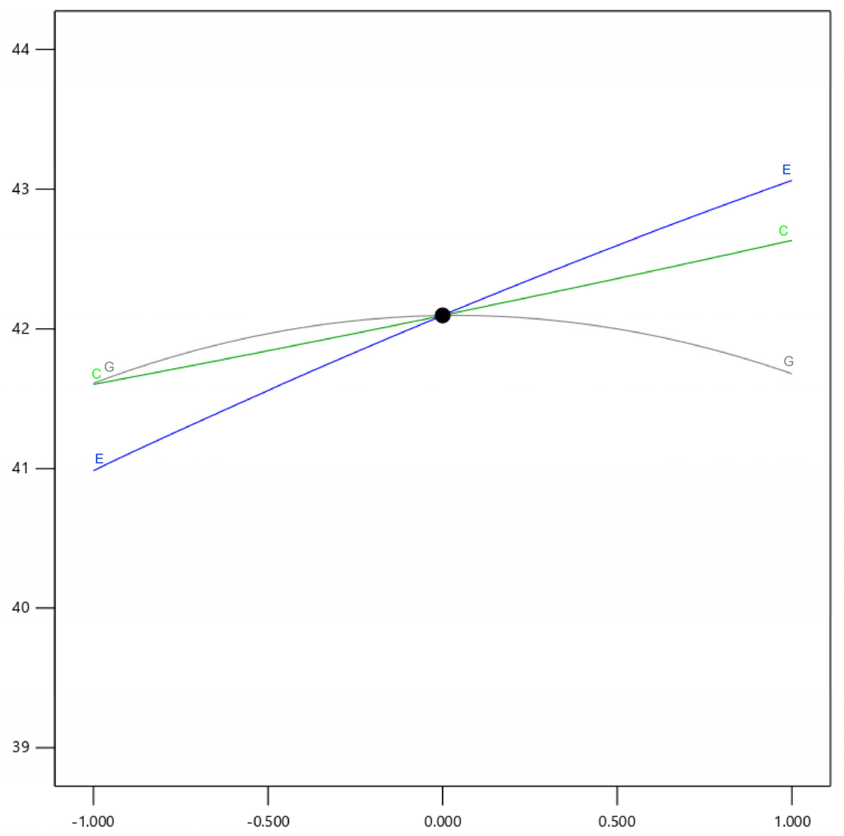
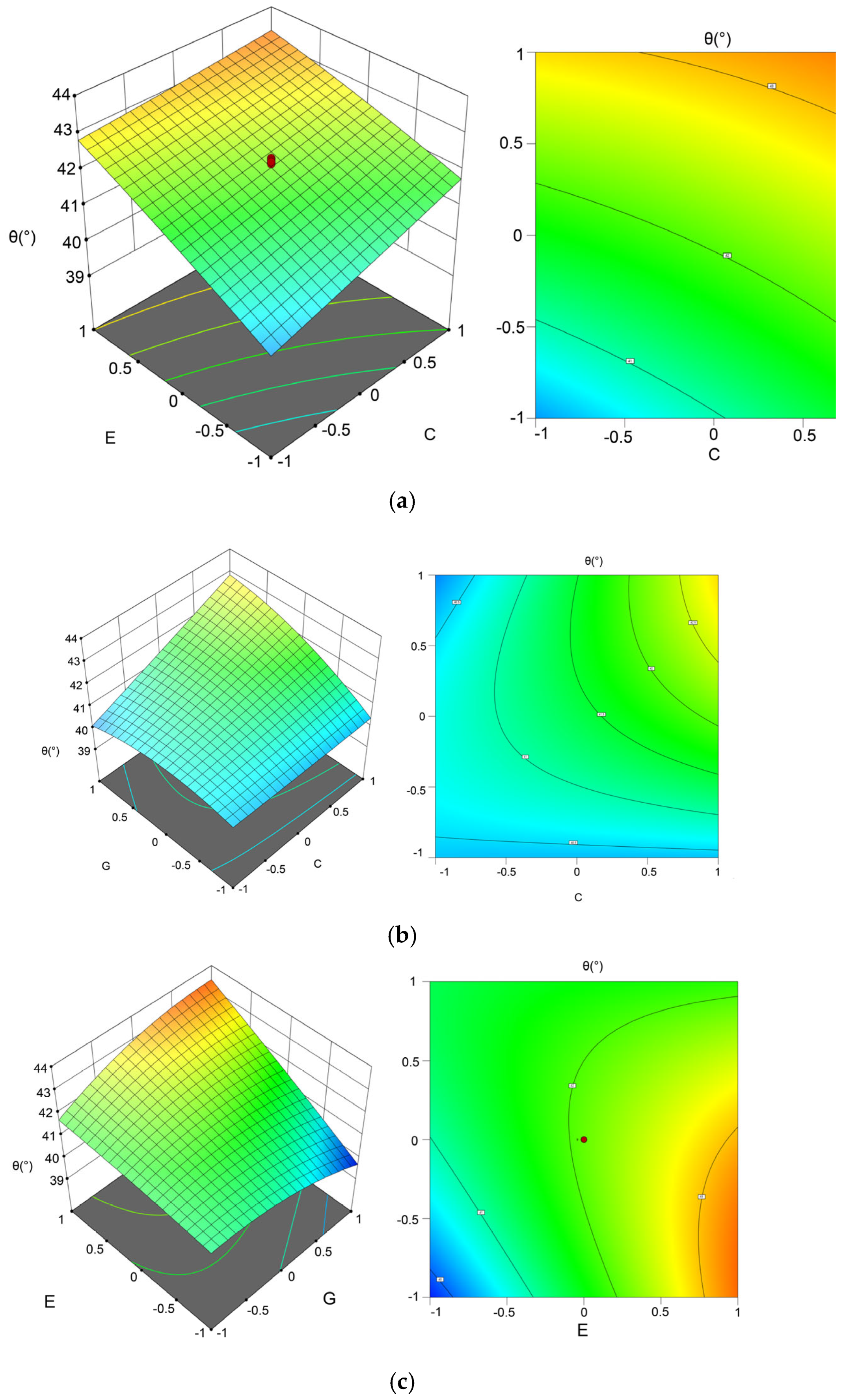
3.4. Interaction Effects of the Regression Model

The perturbation plot (Figure 9) illustrates the differential effects of the three factors (C, E, G) on the angle of repose within their selected ranges. Both rolling friction coefficient (C) and static friction coefficient (E) exhibited positive correlations with the angle of repose, with E demonstrating a steeper slope than C. In contrast, the JKR surface energy (G) displayed a nonlinear relationship: the angle of repose initially increased with rising G but decreased beyond a critical surface energy threshold.

The repose angle of wheat straw feed arises from a dynamic equilibrium among rolling friction, static friction, and surface energy:

• Rolling friction governs local particle rearrangement by dictating energy dissipation during granular adjustments [24].
• Static friction at the straw–steel interface modulates substrate support strength, stabilizing interfacial interactions [25].
• JKR surface energy regulates interparticle adhesion, with cohesive forces dominating at finer scales [26].

Elevated frictional forces amplify the repose angle by restricting particle mobility, while surface energy exhibits a biphasic influence:

• Subcritical Regime: Increased adhesion enhances interparticle cohesion, reducing flowability and elevating the repose angle.
• Supercritical Regime: Excessive agglomeration forms large particle clusters, restructuring the pile geometry and paradoxically improving flowability, thereby decreasing the repose angle.

This mechanistic interplay underscores the necessity of balancing frictional and adhesive parameters to replicate realistic biomass dynamics in DEM simulations.

Based on the regression equation, the response surface and contour plots of the model were established as illustrated in Figure 10.

Figure 10a: At fixed G, the angle of repose (θ) increases monotonically with rising C and E.

Figure 10b: When C transitions from low to high levels, θ shifts from an initial increase-decrease trend to a sustained increase with rising G. Higher G amplifies the positive correlation between C and θ.

Figure 10c: When E transitions from low to high levels, θ transitions from increasing to decreasing with rising G. Higher G diminishes the positive correlation between E and θ

All two-factor interaction terms (C×G, E×G) significantly influenced the angle of repose (p < 0.05), confirming that parameter interdependencies critically shape granular pile dynamics.

3.5. Parameter Optimization via RSM Results

Using Design-Expert software with the actual measured value of wheat straw feed angle of repose (42.3°) as the target, we utilized the Optimization-Numerical module to perform optimization solutions for the regression model [27], with the optimization constraints set as:

$$\left\{\begin{array}{l}\theta \to 42.3°\\ s\left\{\begin{array}{l}0.14\le C\le 0.29\\ 0.43\le E\le 0.53\\ 0.01\le G\le 0.11\end{array}\right.\end{array}\right.$$

(14)

Multiple sets of simulated angles of repose for wheat straw feedstock were obtained through numerical optimization. The parameter combination closest to the physical experimental results comprised the following:

• Kinetic friction coefficient between wheat straw particles: 0.19;
• Static friction coefficient between wheat straw and steel plate: 0.47;
• JKR surface energy: 0.04 J/m².

Based on the comprehensive parameters in Table 4, the data was imported into EDEM 2023 software for simulation, and the simulated angle of repose was 40.95°, yielding a relative error of 3.2% compared to the physical experimental value (42.3°).

4. PSO Based on the PSO-BP Model

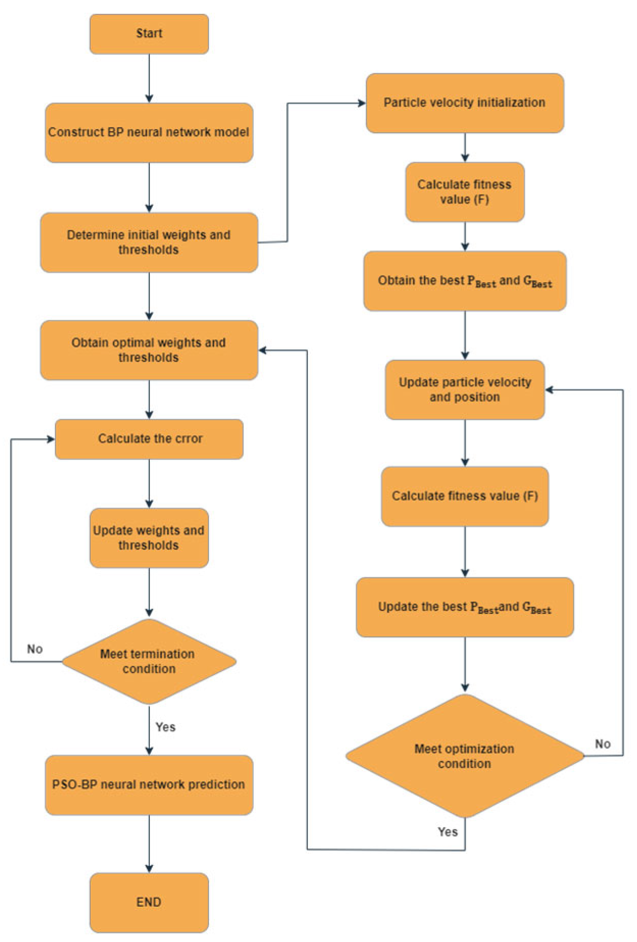
4.1. PSO-BP Description

The particle swarm optimization (PSO) algorithm is a metaheuristic approach grounded in swarm intelligence, drawing inspiration from the collective foraging behaviors of biological populations—such as bird flocks or fish schools—in complex environments [28]. By mimicking the decentralized decision-making and dynamic coordination observed in these natural systems, PSO iteratively refines candidate solutions through social interaction and individual experience. This synergy enables efficient exploration of high-dimensional solution spaces, making it particularly effective for optimizing nonlinear, multimodal problems in fields ranging from agricultural engineering to materials science. In this algorithm, each candidate solution is abstracted as a particle with multidimensional attributes. These particles collectively achieve global optimization through iterative information exchange between individual experiences and swarm intelligence [29]. Specifically, each particle in the solution space possesses dynamically updated position and velocity vectors: The position vector (xi) represents the current solution’s quality, encoding parameter values (e.g., friction coefficients, surface energy); The velocity vector (vi) dictates the search direction and step size, balancing exploration (global search) and exploitation (local refinement).

During the iterative process, particles adhere to three core rules:

• Individual Experience Memory Mechanism: Retention of the particle’s historical optimal position (p_best).
• Swarm Information Sharing Mechanism: Tracking of the swarm’s global optimal position (g_best).
• Motion Inertia Preservation Mechanism: Balancing exploration (global search) and exploitation (local refinement) through velocity damping [30].

Compared to traditional backpropagation (BP) neural networks, the PSO-BP hybrid model achieves synergistic optimization of network parameters through the integration of swarm intelligence optimization mechanisms. Traditional BP networks rely on gradient descent for parameter adjustment, which is prone to converging on local optima and exhibits high sensitivity to initial values [31]. In contrast, the PSO-BP model maps neural network weights and thresholds into the multidimensional solution space of a particle swarm, enabling global exploration of the parameter space through collaborative search mechanisms. This novel hybrid architecture endows the network with three key optimization characteristics:

• Adaptive Parameter Adjustment: Reduces dependency on initial values by dynamically tuning learning rates and momentum terms.
• Balanced Search Strategy: Maintains equilibrium between local refinement (exploitation) and global exploration via velocity-controlled particle dynamics.
• Enhanced Robustness and Generalization: Improves tolerance to noisy or incomplete datasets while minimizing overfitting risks.

According to the study of [32], the hybrid model significantly outperforms traditional methods in metrics such as convergence speed and classification accuracy, with particularly prominent advantages when handling nonlinear complex systems.

4.2. PSO-BP Model Development

PSO-BP neural network model optimization process is shown in Figure 11. The construction steps are as follows:

• Data preprocessing and model construction: First, normalize the input data. Subsequently, construct a backpropagation neural network (BPNN) model, define its network topology (including the number of nodes in the input layer, hidden layer, and output layer), and randomly initialize the connection weights and neuron thresholds.
• PSO hyperparameter configuration: Set key operational parameters for the particle swarm optimization (PSO) algorithm, including maximum iteration count, particle population size (m), individual cognitive factor (c₁), social learning factor (c₂), and inertia weight coefficient controlling search capability.
• Particle swarm initialization: Randomly generate initial positions of the particle swarm within the solution space dimensions corresponding to the BPNN parameters to be optimized (i.e., all weights and thresholds). Simultaneously, assign initial velocities to each particle and constrain their velocity variation range (setting maximum and minimum velocity values).
• Initial fitness evaluation: Initiate the PSO process. Based on each particle’s initial position (representing a set of BPNN parameters), compute its corresponding fitness value (typically the reciprocal or negative value of BPNN prediction error on the validation set). Evaluate the quality of the solution represented by each particle according to this fitness value.
• Enter the iterative loop process. In each iteration:

Update each particle’s personal historical best position (P_best): if the current position’s fitness surpasses its historical best, update P_best.

Update the global historical best position (G_best) of the entire population: if a particle’s Pbest fitness surpasses the current G_best, update G_best.

Adjust each particle’s state according to the following velocity-position update formula [33]:

$$\begin{gathered} V_{ij}^{k+1}=w{V}_{ij}^k+c_1{r}_1\left(P_{IJ}^k-X_{ij}^k\right)+c_2{r}_2\left(G_j^k-X_{ij}^k\right) \\ {X}_{ij}^{k+1}=X_{ij}^k+V_{ij}^{k+1},1\le i\le n,1\le j\le d \end{gathered}$$

(15)

where

k: Iteration count;

w: Inertia weight coefficient;

c₁, c₂: Learning factors (individual/social);

r₁, r₂: Random numbers (for introducing randomness);

P_ij^k: Dimension j of the best position vector found by particle i at iteration k;

G_j^k: Dimension j of the global best position at iteration k;

X_ij^k: Dimension j of the position vector of particle i at iteration k;

V_ij^k+1: Dimension j of the velocity vector of particle i at iteration (k + 1).

Termination condition: The PSO stops when the iteration reaches the preset maximum count or when the particle swarm finds a global optimal solution satisfying the preset fitness threshold.

6.

Constructing the optimization model: Populate the BP neural network model built in Step 1 with the optimal combination of weight and threshold parameters output from the PSO process, thereby obtaining the enhanced-performance PSO-BP hybrid prediction model.

4.3. Model Parameter Setting and Data Processing

4.3.1. Data Preparation and Preprocessing

• This study used the key significant parameters screened by the central composite response surface experiments in Table 10 as the total data (23 sets), performing stratified random sampling into training, validation, and test sets [34]. The training set was used for model parameter learning, the validation set was used for hyperparameter tuning and preventing overfitting, and the test set was used for the final generalization capability evaluation. Among these, the training set comprised 17 sets, the validation set 3 sets, and the test set 3 sets, accounting for approximately 70%, 15%, and 15% of the total data, respectively.
• Data normalization

As shown in

Table 12. Significance parameter normalization.

Parameter	Original	Range Normalized
Straw–straw rolling friction coefficient	[0.14, 0.20]	[0, 1]
Straw–steel static friction coefficient	[0.43, 0.47]	[0, 1]
JKR surface energy (J·m2)	[0.01, 0.05]	[0, 1]

, the input variables undergo feature scaling and are normalized to the [0, 1] range using Min-Max normalization:

$$x_{norm}={\displaystyle \frac{x-x_{min}}{x_{max}-x_{min}}}$$

(16)

The output variable is the angle of repose value, maintaining the original unit (degree).

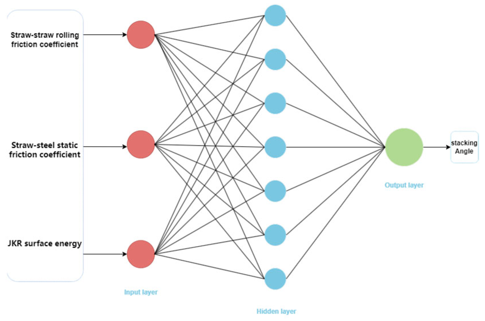
4.3.2. Network Architecture Design

• BP Neural Network Architecture Determination

A three-layer feedforward network was adopted as shown in Figure 12, comprising an input layer, a hidden layer, and an output layer. The core of neural network modeling lies in determining the weight configurations between the hidden layer and output layer, a process fundamentally based on supervised learning for parameter optimization. Given initial weights, input independent variables (wheat straw contact parameters) undergo forward propagation through the network to generate pile angle predictions. Errors are calculated by comparing predictions with measured values, triggering backpropagation to adjust weight parameters. Forward propagation computes the mapping from input to output, while backpropagation iteratively updates weights based on error gradients. One forward–backward propagation cycle constitutes a training iteration; through multiple iterations, predictions gradually converge toward true values. Weight updates during backpropagation rely on the error function and the “gradient descent” method. Related mathematical proofs involving partial differentiation, matrix operations, etc., are complex and lengthy, and have been fully derived elsewhere (omitted in this paper).

This study configured the input layer with significant parameters screened through Plackett–Burman experiments in Section 3.1 (rolling friction coefficient between wheat straw forage particles, static friction coefficient between wheat straw forage and steel plate, JKR surface energy). Thus, the number of input neurons was n1 = 3. The output layer consisted of the dependent variable (pile angle). Through preliminary modeling experiments, the hidden layer neuron count was set to 7. The trainlm function was selected as the training function for the BP neural network, and the ReLU function was chosen as the hidden layer activation function, forming a 3 × 7 × 1 three-layer BP neural network.

2.

Regularization Configuration

Dropout layer: Dropout rate 0.2;

L2 weight penalty: Coefficient λ = 0.001.

4.3.3. Key Parameter Configuration for PSO Algorithm

• Swarm size: 50 particles;
• Maximum iterations: 100;
• Learning factors: c1 = 2.0 → 1.5 (dynamic decay), c2 = 1.5 → 2.0 (dynamic increment);
• Maximum velocity: Vmax = 0.2;
• Inertia weight: w = 0.9 → 0.4 (linear decay).

4.4. Model Evaluation Metrics

The mean squared error (MSE) metric was employed to evaluate the accuracy of the neural network. A lower MSE value indicates higher model precision [35], calculated as follows:

$$MSE={\displaystyle \frac{1}{N}}{{\displaystyle {\sum }_{i=1}^N\left(y_i-{\hat{y}}_i\right)}}^2$$

(17)

where

y_i: the true value;

${\hat{y}}_i$: the predicted value;

N: the total number of data points.

4.5. Results and Analysis

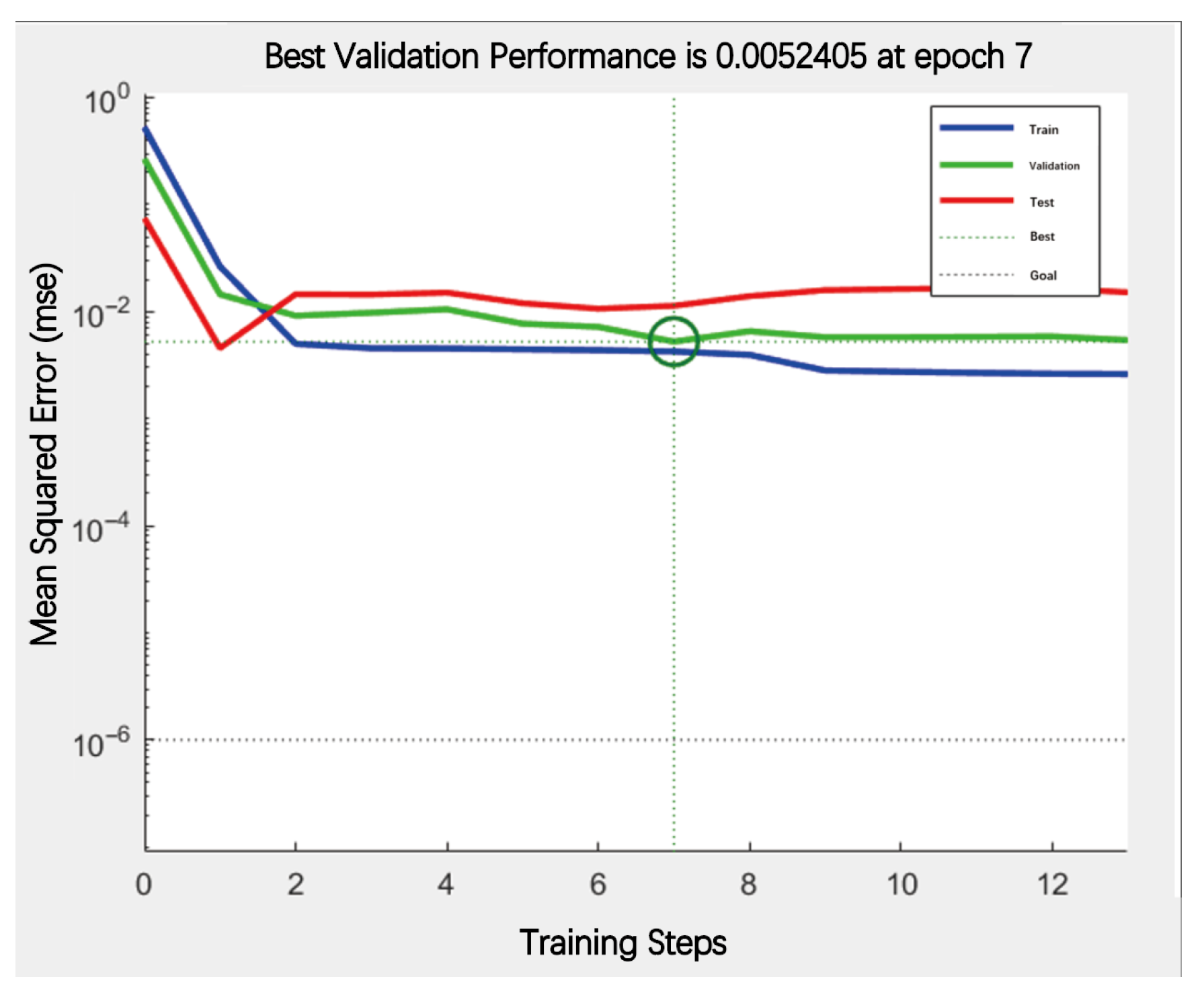
4.5.1. MSE Evaluation of the PSO-PB Model

As the training cycles increased, the MSE of the training, validation, and test groups was used for performance evaluation, as shown in Figure 13. The optimal validation performance (MSE = 0.0052405) was achieved at the seventh training cycle, indicating successful training of the PSO-BP neural network. This network exhibits high fitting accuracy, fast convergence, and strong stability, meeting experimental requirements.

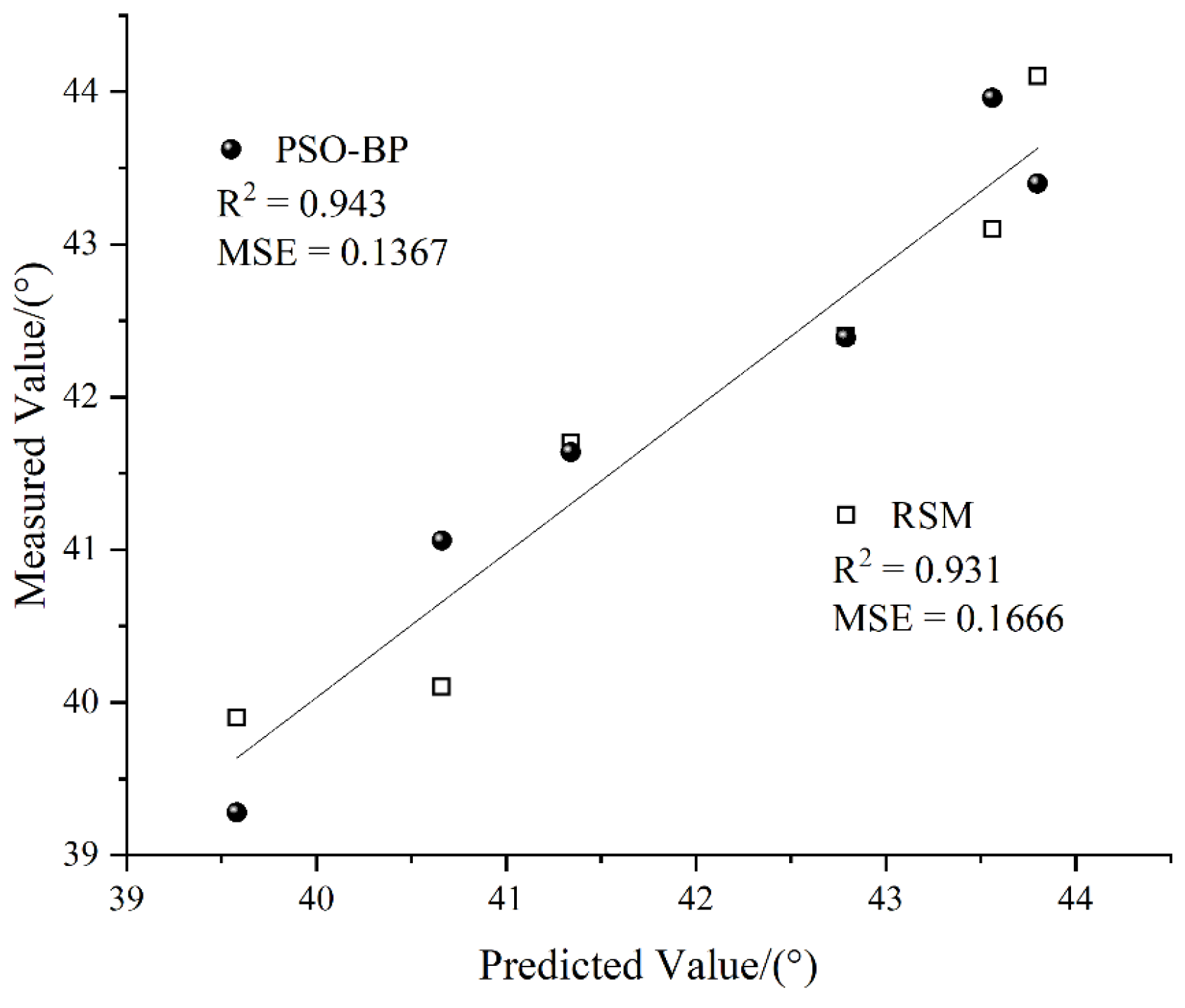
4.5.2. PSO-BP Model Correlation Coefficient Evaluation

As shown in Figure 14, the correlation coefficients between predicted outputs and target values were calculated for the training set, validation set, test set, and full dataset: coefficient of determination (R) for training set = 0.97782, validation set = 0.98134, test set = 0.99447, full dataset = 0.96626. Results indicate all R-values approach 1, demonstrating a highly linear relationship between neural network outputs and expected values. This statistical feature confirms the effective construction of the PSO-BP model and its robust predictive performance, proving its suitability for subsequent experimental analysis.

4.5.3. PSO-PB Parameter Optimization

As shown in Figure 15, the fitness curve of the PSO-BP neural network model varies with the number of iterations. The lower the fitness value, the smaller the prediction error of the model. The curve can be categorized into three distinct phases:

Initial Rapid Decline Phase:

The global search capability of PSO rapidly locates potential optimal regions, with the particle swarm broadly exploring the solution space to identify promising areas.

Intermediate Slow Convergence Phase:

Particles transition to local exploitation, gradually focusing on neighborhoods near optimal solutions. Competition between individual best (p_best) and global best (g_best) positions leads to iterative probing within local regions.

Final Stable Convergence Phase:

The swarm converges near the global optimum, with velocity and position updates approaching zero. A subsequent BP fine-tuning phase applies gradient descent to refine the PSO-derived parameters, further minimizing errors.

Upon reaching the target iteration count (100), the optimal parameters were determined as:

• Kinetic friction coefficient (straw–straw): 0.17;
• Static friction coefficient (straw–steel): 0.46;
• JKR surface energy: 0.03 J/m².

The simulated angle of repose under these parameters was 41.67°, yielding a relative error of 1.5% compared to the experimental value (42.3°).

4.5.4. Comparison of RSM and PSO-BP Optimization Methods

Both response surface methodology (RSM) and the PSO-BP model exhibited prediction errors for the angle of repose below 5%, confirming the accuracy and reliability of optimized parameters for rolling friction coefficient, static friction coefficient, and JKR surface energy. This indicates that both methods are suitable for angle of repose prediction [33]. However, the PSO-BP model demonstrated superior prediction accuracy, with a post-optimization error (1.5%) significantly lower than RSM (3.2%). As shown in Figure 16, both models displayed strong fitting precision between measured and predicted values. The evaluation metrics of the PSO-BP model (R² = 0.943, MSE = 0.1367) outperformed RSM (R² = 0.931, MSE = 0.1666), with R² increasing by 1.29% and MSE decreasing by 17.95%. This confirms the PSO-BP model’s enhanced predictive capability and higher accuracy over RSM.

4.5.5. Discrete Element Simulation Verification Experiment

Using the optimal solution obtained from the aforementioned PSO-BP model, EDEM simulation was again performed on wheat straw forage. As shown in Figure 17, the contour angles show no significant difference between the simulation test and the physical test, indicating the accuracy of the optimized parameters. The wheat straw forage model and parameter calibration results established in this study can be applied to discrete element simulation research.

5. Conclusions

• Systematically measured eight key physical parameters of wheat straw forage (moisture content 11.59%, bulk density 45.82 kg/m³, friction coefficient, restitution coefficient, etc.), establishing the first discrete element basic characteristic database for long-fiber materials, filling the gap in this field.
• Established a discrete element simulation model based on the Hertz–Mindlin with JKR cohesion contact model. Using PB experiments and steepest ascent tests, three significant parameters affecting the angle of repose were screened. Central composite response surface design in RSM was employed for experimental analysis, further optimizing the significant parameters. Optimized results: dynamic friction coefficient between wheat straw forage particles = 0.19, static friction coefficient between wheat straw forage and steel plate = 0.47, JKR surface energy = 0.04 J/m². The simulated wheat straw angle of repose was 40.95°, with a relative error of 3.2% compared to the actual physical angle of repose.
• Intelligent calibration innovation: We proposed a PSO-BP fusion optimization framework, utilizing swarm intelligence algorithms to globally search neural network weights. This solved the problem of traditional RSM easily falling into local optima during high-dimensional nonlinear optimization. We obtained optimal parameters: dynamic friction coefficient between wheat straw forage particles = 0.17; static friction coefficient between wheat straw forage and steel plate = 0.46; and JKR surface energy = 0.03 J/m². The simulated angle of repose was 41.67°, with a relative error of 1.5% compared to the actual angle of repose.
• Accuracy and efficiency breakthrough: The PSO-BP model reduced the angle of repose prediction error to 1.5% (versus 3.2% for RSM), representing a 53.13% error reduction. Optimized parameters can be directly imported into EDEM software to guide feeding machinery design. Expected to reduce blockage failures by approximately 20%.
• Although this study achieved breakthroughs in static parameter calibration for wheat straw (error reduced by 53.13%), limitations remain, such as weak environmental adaptability and insufficient real-time performance. Future work will extend the research to materials like corn straw and rice straw through dynamic compensation model development, algorithm hardware acceleration, and multi-crop validation. A cloud platform for straw material calibration will be established to enhance the framework’s engineering universality and promote field application. Ultimately, a full-chain solution of “parameter calibration–simulation optimization–equipment control” will be built to support intelligent upgrading in animal husbandry.

References

1. Cheng, M.; Yao, W. Trend prediction of carbon peak in China’s animal husbandry based on the empirical analysis of 31 provinces in China. Environ. Dev. Sustain. 2024, 26, 2017–2034. [Google Scholar] [CrossRef]
2. Yang, Y.; Wang, H.; Li, C.; Liu, H.; Fang, X.; Wu, M.; Lv, J. Identification of the soil physicochemical and bacterial indicators for soil organic carbon and nitrogen transformation under the wheat straw returning. PLoS ONE 2024, 19, e0299054. [Google Scholar] [CrossRef] [PubMed]
3. Sufyan, A.; Ahmad, N.; Shahzad, F.; Embaby, M. Improving the nutritional value and digestibility of wheat straw, rice straw, and corn cob through solid state fermentation using different Pleurotus species. J. Sci. Food Agric. 2022, 102, 2445–2453. [Google Scholar] [CrossRef]
4. Guo, J.; Lyu, J. The digital economy and agricultural modernization in China: Measurement, mechanisms, and implications. Sustainability 2024, 16, 4949. [Google Scholar] [CrossRef]
5. Zhao, J.J.; Zhang, G.C.; Wu, H.; Li, X.C.; Zhang, Q.; Lou, Y.Z.; Li, H.Q.; Xu, B.; Mu, G. Calibration and simulation of discrete element contact parameters for Ruditapes philippinarum shallow-sea aquaculture substrates. Trans. Chin. Soc. Agric. Eng. 2025, 41, 295–304. [Google Scholar]
6. Sun, J.B.; Liu, Q.; Yang, F.Z.; Liu, Z.J.; Wang, Z. Calibration of discrete element simulation parameters for interaction between loess plateau slope soil and rotary tillage components. Trans. China Soc. Agric. Mach. 2022, 53, 63–73. [Google Scholar]
7. Du, C.; Han, D.; Song, Z.; Chen, Y.; Chen, X.; Wang, X. Calibration of contact parameters for complex shaped fruits based on discrete element method: The case of pod pepper (Capsicum annuum). Biosyst. Eng. 2023, 226, 43–54. [Google Scholar] [CrossRef]
8. Li, X.; Du, Y.; Liu, L.; Zhang, Y.; Guo, D. Parameter calibration of corncob based on DEM. Adv. Powder Technol. 2022, 33, 103699. [Google Scholar] [CrossRef]
9. Ding, X.T.; Li, K.; Hao, W.; Yang, Q.C.; Yan, F.X.; Cui, Y.J. Calibration of camellia seed simulation parameters based on RSM and GA-BP-GA optimization. Trans. Chin. Soc. Agric. Mach. 2023, 54, 139–150. [Google Scholar]
10. Wang, X.M.; Lyu, J.X.; Li, X.J.; Wu, Y.Q.; Li, X.G.; Hao, X.F.; Qiao, J.Z.; Xu, K. Moisture content prediction in drying process of impregnated bamboo bundles based on PSO-BP neural network model. Sci. Silvae Sin. 2025, 61, 187–198. [Google Scholar]
11. Li, H.; Wu, M.; Wu, J.; Wan, J.; He, Y.; Ding, Y.; Liu, J. The Effect of Dietary Zinc Oxide Nanoparticles on Growth Performance, Zinc in Tissues, and Immune Response in the Rare Minnow (Gobiocypris rarus). Aquac. Nutr. 2024, 2024, 9553278. [Google Scholar] [CrossRef] [PubMed]
12. GB/T 6435-2014; Determination of Moisture in Feedstuffs. Standardization Administration of China (SAC): Beijing, China, 2014.
13. NY/T 1881.6-2010; Test Methods for Densified Biomass Fuel. Ministry of Agriculture and Rural Affairs of China: Beijing, China, 2010.
14. Huo, L.; Meng, H.; Tian, Y.; Zhao, L.; Hou, S. Experimental study on physical property of smashed crop straw. Trans. Chin. Soc. Agric. Eng. 2012, 28, 189–195. [Google Scholar]
15. Trüe, M.; Böttcher, R.; Faßhauer, O.; Aman, S.; Van Wachem, B.; Müller, P. Comparison of measurement systems for free fall tests and calculations of the coefficient of restitution. Meas. Sci. Technol. 2018, 29, 105403. [Google Scholar] [CrossRef]
16. Ma, D.; Shi, S.; Hou, J.; Zhou, J.; Li, H.; Li, J. Calibration and Experimentation of Discrete Elemental Model Parameters for Wheat Seeds with Different Filled Particle Radii. Appl. Sci. 2024, 14, 2075. [Google Scholar] [CrossRef]
17. Boac, J.M.; Ambrose, R.P.K.; Casada, M.E.; Maghirang, R. Applications of discrete element method in modeling of grain postharvest operations. Food Eng. Rev. 2014, 6, 128–149. [Google Scholar] [CrossRef]
18. Qin, D.; Li, M.; Wang, T.; Chen, J.; Wu, H. Design and mechanical properties of negative poisson’s ratio structure-based topology optimization. Appl. Sci. 2023, 13, 7728. [Google Scholar] [CrossRef]
19. Xu, T.; Gou, Y.; Huang, D.; Yu, J.; Li, C.; Wang, C. Modeling and Parameter Selection of the Corn Straw–Soil Composite Model Based on the DEM. Agriculture 2024, 14, 2075. [Google Scholar] [CrossRef]
20. Schramm, M.; Tekeste, M.Z. Wheat straw direct shear simulation using discrete element method of fibrous bonded model. Biosyst. Eng. 2022, 213, 1–12. [Google Scholar] [CrossRef]
21. Shi, Y.W.; Niu, X.X.; Yang, H.M.; Chu, M.; Wang, N.; Bao, H.F.; Zhan, F.Q.; Yang, R.; Lpu, K. Optimization of the fermentation media and growth conditions of Bacillus velezensis BHZ-29 using a Plackett–Burman design experiment combined with response surface methodology. Front. Microbiol. 2024, 15, 1355369. [Google Scholar] [CrossRef]
22. Zhang, X.; Wang, H.; Wang, F.; Lian, Z. Parameter calibration of discrete element model for alfalfa seeds based on EDEM simulation experiments. Int. J. Agric. Biol. Eng. 2024, 17, 33–38. [Google Scholar] [CrossRef]
23. Yuan, J.; Wang, J.; Li, H.; Qi, X.; Wang, Y.; Li, C. Optimization of the cylindrical sieves for separating threshed rice mixture using EDEM. Int. J. Agric. Biol. Eng. 2022, 15, 236–247. [Google Scholar] [CrossRef]
24. Song, X.; Dai, F.; Zhang, F.; Wang, D.; Liu, Y. Calibration of DEM models for fertilizer particles based on numerical simulations and granular experiments. Comput. Electron. Agric. 2023, 204, 107507. [Google Scholar] [CrossRef]
25. Li, Y.; Wei, D.; Zhang, N.; Fuentes, R. Effect of basal friction on granular column collapse. Granul. Matter 2024, 26, 62. [Google Scholar] [CrossRef]
26. Teng, Y.L.; Wu, X.L.; Yang, S.P.; Li, S.H.; Zhang, C.Q. Calibration and verification of DEM parameters for asphalt mixture based on experimental design method and bulk experiments. Part. Sci. Technol. 2025, 43, 327–337. [Google Scholar] [CrossRef]
27. Yang, L.; Chen, W.; Kan, Z.; Meng, H.; Qi, J. Parameter calibration for discrete element simulation of Leymus chinensis seeds based on RSM optimization. Sci. Rep. 2025, 15, 7947. [Google Scholar] [CrossRef]
28. Jain, M.; Saihjpal, V.; Singh, N.; Singh, S.B. An overview of variants and advancements of PSO algorithm. Appl. Sci. 2022, 12, 8392. [Google Scholar] [CrossRef]
29. Tharwat, A.; Schenck, W.A. conceptual and practical comparison of PSO-style optimization algorithms. Expert Syst. Appl. 2021, 167, 114430. [Google Scholar] [CrossRef]
30. Wang, M.; Lu, Z.; Wan, W.; Zhao, Y. A calibration framework for the microparameters of the DEM model using the improved PSO algorithm. Adv. Powder Technol. 2021, 32, 358–369. [Google Scholar] [CrossRef]
31. Ma, X.; Guo, M.; Tong, X.; Hou, J.; Liu, H.; Ren, H. Calibration of small-grain seed parameters based on a BP neural network: A case study with red clover seeds. Agronomy 2023, 13, 2670. [Google Scholar] [CrossRef]
32. Li, Y.; Zhou, L.; Gao, P.; Yang, B.; Han, Y.; Lian, C. Short-term power generation forecasting of a photovoltaic plant based on PSO-BP and GA-BP neural networks. Front. Energy Res. 2022, 9, 824691. [Google Scholar] [CrossRef]
33. Li, S.; Fan, Z. Evaluation of urban green space landscape planning scheme based on PSO-BP neural network model. Alex. Eng. J. 2022, 61, 7141–7153. [Google Scholar] [CrossRef]
34. Wang, P.; Qiao, H.; Feng, Q.; Xue, C.; Zhang, Y. Water resistance prediction of magnesium oxychloride cement concrete based on PSO-BPNN model. J. Build. Mater. 2024, 27, 189–196. [Google Scholar]
35. Su, R.; Ge, Y.; Lin, Y. Temperature-compensated hollow-core fiber Fabry-Perot strain sensor based on optimized PSO-BP. Acta Phys. Sin. 2025, 74, 1–20. [Google Scholar]
Figure 1. Wheat straw feed.
Applsci 15 07668 g001
Figure 3. Experimental setup for measuring the coefficient of restitution: 1. Steel ruler; 2. Computer; 3. High-speed camera; 4. Light source; 5. Steel plate.
Applsci 15 07668 g003
Figure 4. Stacking angle physical test. Note: 1. Universal material tension and pressure testing machine; 2. Fixture; 3. Cylinder; 4. Stacking angle; 5. High-definition camera; 6. Computer.
Applsci 15 07668 g004
Figure 5. Stacking-angle image processing. (a) Original image; (b) Grayscale processing; (c) Binarization; (d) Edge profile extraction; (e) Contour pixel point coordinates.
Applsci 15 07668 g005
Figure 6. Silage corn components and discrete element particle models.
Applsci 15 07668 g006
Figure 7. Schematic representation of the JKR cohesive contact model.
Applsci 15 07668 g007
Figure 8. Stacking-angle simulation test. (a) Feed dispersal process; (b) feed dispersal process.
Applsci 15 07668 g008
Figure 9. Perturbation.
Applsci 15 07668 g009
Figure 10. Contour and surface maps of the interaction factors. (a) C–E interaction diagram; (b) C–G interaction diagram; (c) E–G interaction diagram.
Applsci 15 07668 g010
Figure 11. Optimization process of the PSO-BP neural network model.
Applsci 15 07668 g011
Figure 12. Construction of the backpropagation (BP) neural network model.
Applsci 15 07668 g012
Figure 13. Performance.
Applsci 15 07668 g013
Figure 14. Regression analysis.
Applsci 15 07668 g014
Figure 15. Fitness evolution curve of the particle swarm optimization process.
Applsci 15 07668 g015
Figure 16. Predicted and measured values of RSM and PSO-BP methods.
Applsci 15 07668 g016
Figure 17. Comparison of physical and simulation tests.
Applsci 15 07668 g017