A Finite Element Approach to the Upper-Bound Bearing Capacity of Shallow Foundations Using Zero-Thickness Interfaces

Abstract

This study presents a robust numerical framework for evaluating the upper-bound ultimate bearing capacity of shallow foundations in cohesive and C-phi soils using a self-developed finite element method. The model incorporates multi-segment zero-thickness interface elements to accurately simulate soil discontinuities and progressive failure mechanisms, based on the Mohr–Coulomb failure criterion. In contrast to optimization-based methods such as discontinuity layout optimization (DLO) or traditional finite element limit analysis (FELA), the proposed approach uses predefined failure mechanisms to improve computational transparency and efficiency. A variety of geometric failure mechanisms are analyzed, including configurations with triangular, circular, and logarithmic spiral slip surfaces. Particular focus is given to the transition zone, which is discretized into multiple blocks to enhance accuracy and convergence. The method is developed for two-dimensional problems under the assumption of elastic deformable-plastic behavior and homogeneous isotropic soil, with limitations in automatically detecting failure mechanisms. The proposed approach is validated against classical theoretical solutions, demonstrating excellent agreement. For friction angles ranging from 0° to 40°, the computed bearing capacity factors N_c and N_q show minimal deviation from the analytical results, with errors as low as 0.04–0.19% and 0.12–2.43%, respectively. The findings confirm the method’s effectiveness in capturing complex failure behavior, providing a practical and accurate tool for geotechnical stability assessment and foundation design.

1. Introduction

The accurate assessment of the ultimate bearing capacity of shallow foundations is critical for ensuring the safety, reliability, and cost-effectiveness of civil infrastructure. In geotechnical engineering, this problem has been extensively studied through various analytical and numerical methods [1]. Traditional approaches generally fall into four categories: limit equilibrium methods [2,3,4,5], slip line methods [6,7,8], limit analysis methods [9,10,11,12], and numerical methods, such as finite element or finite difference methods [13,14,15].

Classical bearing capacity theories developed by Terzaghi [2], Meyerhof [3], and Vesic [4] offer simple, closed-form solutions based on idealized assumptions. While these solutions remain widely used in practice, they are often inadequate for addressing complex conditions involving heterogeneous soils, irregular geometries, and nonlinear soil-structure interactions.

The limit analysis offers a more rigorous theoretical framework by directly evaluating collapse loads without modeling the full-load deformation behavior. Based on the assumption of elastic–perfectly plastic material behavior, the upper and lower bounds of a system’s load-bearing capacity depend on the chosen internal failure mechanisms and equilibrium constraints [16,17,18,19]. The upper-bound theorem, in particular, estimates the maximum load a structure can sustain using kinematically admissible velocity fields and plastic dissipation. This approach has been extensively applied to geotechnical stability problems involving foundations, slopes, and retaining structures [20,21].

In upper-bound limit analysis, it is essential to define a compatible failure mechanism whose geometry satisfies the principles of energy dissipation and external work. For cohesive soils, failure mechanisms typically comprise straight or circular slip surfaces, while for C-phi soils, mechanisms may include logarithmic spirals. The assumed failure geometry must closely reflect realistic collapse patterns to ensure that the estimated bearing capacity approximates actual behavior [22,23,24].

A key challenge in upper-bound limit analysis is the accurate representation of failure mechanisms. The assumed geometry must conform to realistic collapse patterns to ensure reliable capacity estimates, particularly in soils exhibiting cohesion and internal friction [22,23,24]. Although modern finite element limit analysis has enhanced the flexibility and accuracy of upper-bound methods, difficulties remain in capturing localized failures such as slip surfaces, cracks, and detachment at interfaces [22,25,26].

To overcome these limitations, zero-thickness interface elements have been introduced. These elements allow for displacement discontinuities and frictional sliding, making them well suited for modeling stress transfer across soil layers and soil–structure boundaries. When coupled with classical plasticity models, like Mohr–Coulomb, they offer a more realistic depiction of interfacial behavior under failure conditions [27,28]. Recent advancements in automatic collapse mechanism identification have introduced robust optimization-based strategies. Discontinuity layout optimization (DLO), as proposed by Smith and Gilbert [29], offers a direct and efficient means to evaluate upper-bound solutions without assuming predefined failure paths. This method has been further advanced through open source implementations [30] and adaptive strategies [31], which allow for complex geometries and stress fields to be considered in a fully automated way.

Finite element limit analysis (FELA) is a powerful numerical method used to estimate the ultimate load-bearing capacity of geotechnical systems without performing full stress–strain simulations. Based on the plasticity theory, FELA provides rigorous upper- or lower-bound solutions to collapse loads. In upper-bound FELA, kinematically admissible failure mechanisms are analyzed to compute collapse loads through optimization. The use of zero-thickness interface elements has significantly improved the modeling of discontinuities and failure surfaces, especially in soils governed by the Mohr–Coulomb criterion. These elements allow for the accurate simulation of progressive failure and localized shear bands. Advanced approaches, such as those introduced by Krabbenhøft et al. [25], automate mechanism identification using optimization algorithms and have set a benchmark in the field.

Accurately evaluating the ultimate bearing capacity of shallow foundations is essential for safe and cost-effective geotechnical designs. While analytical methods offer insights under idealized conditions, numerical approaches are better suited for complex problems. However, methods like discontinuity layout optimization (DLO) and traditional finite element limit analysis (FELA) often face challenges, such as convergence instability, mesh sensitivity, and limited scalability. Moreover, adaptive failure detection methods can obscure physical interpretation and demand high computational effort. This study addresses these limitations by exploring a structured finite element approach with predefined failure mechanisms and zero-thickness interface elements. It is guided by two questions: (1) Can such a model match the accuracy of traditional upper-bound methods? (2) How well does it balance computational efficiency with the ability to capture progressive failure in cohesive and C-phi soils?

This study presents a numerical framework based on a self-developed finite element program that incorporates zero-thickness interface elements governed by the Mohr–Coulomb failure criterion. The model assumes a homogeneous, isotropic, linearly elastic soil mass with predefined failure surfaces. A series of parametric studies is conducted to examine how different failure geometries influence the predicted bearing capacity.

By integrating mesh optimization with upper-bound limit analysis, the proposed method yields accurate and computationally efficient estimations of collapse loads. The results not only validate the effectiveness of the approach, but also highlight its potential for simulating progressive failure mechanisms with high fidelity. Finally, this research contributes a reliable tool for geotechnical design and offers a practical pathway to integrating discontinuity modeling within upper-bound limit analysis for shallow foundations.

2. Upper-Bound Limit Analysis Theorem

According to the upper-bound theorem, if an external load is applied to a system with a kinematically admissible failure mechanism, the rate of external work equals the rate of internal energy dissipation due to plastic deformation. If this balance is achieved, collapse is considered imminent, and the applied load represents an upper estimate of the true failure load. Conversely, the lower-bound theorem states that if a stress field can be found that satisfies equilibrium conditions and no material point exceeds the yield criterion, then the structure remains stable under the applied load. This load then serves as a conservative lower estimate of the actual failure load [16,17,18,19]. Therefore, the principle of the upper limit theory is described as follows:

$$\sum F_u\cdot \delta w_u={\int }_v{\sigma }_u\cdot \delta {\epsilon }_{u}dv$$

(1)

To obtain the upper limit, F_u, of the external load, the internal initial stress, σ_u, the boundary displacement, δw_u, and the internal strain increment, δε_u, are generated along with the external load. The left side (work performed by the external forces) and the right side (work performed by the internal stresses) will be equal; therefore:

$$\sum F_c\cdot \delta w_c={\int }_v{\sigma }_c\cdot \delta {\epsilon }_{c}dv$$

(2)

where F_c and σ_c are the external load and internal initial stress when failure occurs. The subscripts u and c represent the ultimate condition and the failure condition, respectively.

Atkinson (1981) [16] applied the upper- and lower-bound principles of limit analysis to evaluate the ultimate bearing capacity of foundation soils. In his study, soils were classified into two main types: purely cohesive soils and cohesive–frictional (c-phi or c-φ) soils. By analyzing different assumed failure mechanisms, it can be derived for the ultimate bearing capacity corresponding to each soil type and failure geometry. At the limit state, the observed failure mechanisms were found to align with the full shear failure patterns previously described by Vesic (1973) [4]. In the context of upper-bound analysis, particularly for load-induced failure in soils, the classification into cohesive and C-phi soils is essential. This distinction enables the selection of appropriate failure mechanisms and energy dissipation models for accurately estimating collapse loads under varying soil conditions.

2.1. Cohesive Soils

In the upper-bound limit analysis of cohesive soils, an essential first step is to assume a kinematically admissible failure mechanism. The geometry of this mechanism must satisfy the condition that the internal work dissipated along the failure surface (δW) equals the external work performed by the applied loads (δE). For purely cohesive soils (where c = c_u and φ = 0), the assumed failure mechanism can be represented by either straight-line slip surfaces or circular arc slip surfaces. Two common types of failure geometries for cohesive soils are (1) the planar slip surface mechanism, composed of straight-line segments, and (2) the circular slip surface mechanism, defined by arc-shaped failure paths. Any proposed failure mechanism must be physically reasonable and reflect the expected collapse behavior to ensure that the calculated ultimate bearing capacity closely approximates the actual value. In scenarios involving plane strain conditions, deformation is often assumed to be negligible in directions orthogonal to the primary failure mechanism. Thus, the analysis focuses on continuous deformation within the soil mass and discontinuities along the sliding surfaces [16].

The relationship between the internal work conducted on the sliding surface to resist the external force and the displacement increment of the soil caused by the external force is:

$$\delta W=\sum c_{u}L\delta w+\sum 2c_{u}R{\theta }_f\delta w$$

(3)

where the first term δw on the right is the internal stress of the plane sliding surface, and the second term δw on the right is the internal stress of the arc sliding surface; where c_u is the undrained shear strength of the soil on the sliding surface, L is the length of the plane sliding surface, R is the radius of the arc sliding surface, and θ_f is the angle of the arc sliding surface. The external work, δE, generated by an external force or soil weight is expressed as

$$\delta E=\sum \delta \omega F+{\int }_A\delta \omega qdA+{\int }_V\delta \omega \gamma dV$$

(4)

where F is the ultimate bearing capacity above the foundation, q is the surface soil load, γ is the unit weight of the soil, V is the volume of the soil, A is the area under the surface soil load, and δw is the displacement increment caused by soil settlement due to external force.

Assuming the failure mechanism of a shallow foundation occurs within a semi-infinite soil mass, the failure geometry can be represented by a composite mechanism consisting of two triangular zones and a central circular fan zone, as illustrated in Figure 1a. As shown in Figure 1b, the displacement increment resulting from the applied external load corresponds to the vertical settlement of the foundation. This displacement is directly related to the increment in the surface load, q, which drives the assumed failure mechanism. Its geometric relationship is given as

$${\int }_A{\delta \omega }_{q}qdA=-\delta w_{s}qC$$

(5)

where C = B and δw_q = −δw_s; therefore, the work performed by the force on these five sliding surfaces is

$$\delta E=q_{u}B\delta w_q-qC\delta w_q$$

(6)

and

$$\delta W={\pi c}_{u}B\delta w_q$$

(7)

where δW is the sum of the internal work conducted by each line segment on the sliding surface to resist stress. According to the principle of conservation of energy (δW = δE), the ultimate bearing value of the foundation can be obtained as follows.

$$q_u=\left(2+\pi \right)c_u+q$$

(8)

When the overburden pressure q = 0, then

2.2. C-Phi Soils

In the upper-bound limit analysis of cohesive–frictional (C-phi) soils, it is necessary to first assume a kinematically admissible failure mechanism. The geometry of this mechanism must satisfy the condition that the internal work dissipated along the failure surface balances the external work done by applied loads. For C-phi soils, typical failure mechanisms consist of straight-line slip surfaces, spiral curves (such as logarithmic spirals), or a combination of both. To ensure the accuracy of the upper-bound estimation, the assumed failure mechanism should reflect realistic soil behavior under limit conditions. The resulting prediction of ultimate bearing capacity must closely approximate the true collapse load. Under plane strain conditions, deformation in the out-of-plane direction is neglected, and the analysis focuses on the in-plane motion along continuous and discontinuous failure surfaces. Furthermore, the direction of relative displacement along the slip surface is influenced by the dilation angle, which governs the orientation of plastic strain increments and affects the geometry of the assumed failure mechanism.

When assuming a failure mechanism in cohesive–frictional (C-phi) soils, the mechanism must conform to the fundamental characteristics of such materials. Specifically, under the condition of limit equilibrium, the internal work dissipated along the sliding surface in resisting external loads must balance the external work input. In the idealized case where the mechanism is perfectly kinematically admissible and satisfies the yield criterion everywhere, the net virtual work is zero. This relationship can be expressed as

$$\delta W=0$$

(9)

The external work, δE, conducted by the external force or the soil’s weight can be given by

$$\delta E=\sum \delta wF+{\int }_A\delta w\left(q-u\right)dA+{\int }_V\delta w\left(\gamma -{\gamma }_w\right)dV$$

(10)

where F is the ultimate bearing load above the foundation, q is the surcharge pressure, u is the pore water pressure, γ is the unit weight of the soil, γ_w is the unit weight of water, V is the volume of the soil, A is the area under the surcharge, and δw is the displacement increment of the soil settlement caused by external force [16].

The failure mechanism of a shallow foundation on a horizontal surface is illustrated in Figure 2a. This mechanism consists of a sliding surface formed by two triangular zones and a single logarithmic spiral. As shown in Figure 2b, the horizontal displacement increments in sliding zones I and III result from external forces. According to the geometric relationship, if the angle of the sector formed by the logarithmic spiral is 90°, the corresponding spiral equation can be derived as follows:

$$r_b=r_{a}exp\left({\displaystyle \frac{\pi }{2}}tan\phi \right)$$

(11)

Its geometric relationship can be expressed as

$$\delta w_b=\delta w_{a}exp\left({\displaystyle \frac{\pi }{2}}tan\phi \right)$$

(12)

and

$$C=Btan\left(45°+{\displaystyle \frac{\phi }{2}}\right) exp\left({\displaystyle \frac{\pi }{2}}tan\phi \right)$$

(13)

The vertical displacement increment, δw_q, of the ground heave caused by the surcharge pressure, q, can be given as

$$\delta w_q=\delta w_{q_u}tan\left(45°+{\displaystyle \frac{\phi }{2}}\right) exp\left({\displaystyle \frac{\pi }{2}}tan\phi \right)$$

(14)

Assuming that the soil is completely dry (u = γ_w = 0), and ignoring its weight, the external work it performs to resist the external force can be obtained as

$$\delta E=q_{u}B\delta w_{q_u}-qC\delta w_q$$

(15)

The work performed by this force on the sliding surface at the time of failure can be obtained as follows:

$$\delta E=q_u-qtan\left(45°+{\displaystyle \frac{\phi }{2}}\right) exp\left(\pi tan\phi \right)$$

(16)

According to the energy conservation principle (δE = δW), the upper limit of the foundation bearing capacity can be obtained as follows.

3. Theoretical Analysis and Programming of Zero-Thickness Interface Elements

In geotechnical systems, contact surfaces, whether between the foundation and the soil or between different soil layers, serve as discontinuity surfaces or interfaces. Traditional analysis methods, such as the limit equilibrium method, often neglect these interfaces and their influence. However, the presence of discontinuities can significantly affect the overall engineering behavior and should not be ignored. Interface elements are generally categorized into two types: zero-thickness (thickness-free) interface elements [27,28] and finite-thickness interface elements [32,33]. This study adopts the four-node, zero-thickness interface element originally proposed by Day and Potts (1994) [28] as the theoretical foundation. Building on this, a modified six-node isoparametric interface element is introduced, and its influence on the analysis results is examined and discussed.

Zero-thickness interface elements are standard in geotechnical FEM for slip surfaces and joints, typically enforced with penalty or augmented-Lagrangian traction–separation laws. Our multi-segment Mohr–Coulomb interface follows the same paradigm. For context, PLAXIS uses zero-thickness interfaces with normal and shear stiffness and a Coulomb envelope [34]; we adopt identical stiffness definitions but embed the elements along predefined slip paths, assigning stiffness from the minimum Young’s modulus of adjoining materials to avoid locking (a convention also used by PLAXIS). ABAQUS [35] cohesive/contact pairs likewise implement traction–separation behavior; we apply the zero-thickness ideal-plastic limit directly, which is well suited to upper-bound collapse analysis. Comparable formulations have proven accurate in prior studies on footing and slope stability [36,37].

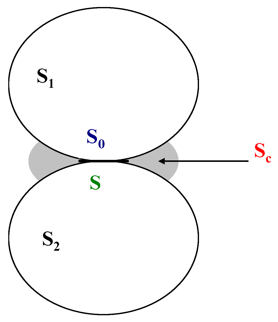
3.1. Zero-Thickness Interface Model

To simulate the mechanical behavior at the interface between two adjacent soil bodies, this study employs multi-segment, zero-thickness interface elements. The contact mechanics between two adjacent objects can generally be categorized into three types [38]: (1) Fully bonded contact: There is neither separation nor frictional resistance along the interface; the two bodies behave as a single, continuous entity. The stress–strain transfer in this case is linear and reversible. (2) Frictionless sliding: Relative sliding occurs at the interface without frictional resistance. This results in a nonlinear but still reversible stress-strain response. (3) Frictional sliding: Relative displacement occurs along the interface with frictional resistance present. This represents a more complex scenario with a nonlinear and irreversible stress–strain transfer mechanism.

When two objects, S₁ and S₂, come into contact, the thinking mode can be seen in Figure 3, where S_c is the potential sliding surface, S is the actual contact surface, and S₀ is the initial contact surface. In the absence of an external force, the initial contact surface S = S₀ is the actual contact surface; when two objects slide but do not separate under the action of external force (that is, S₀ < S < S_c), the actual contact surface is between the initial contact surface and the potential sliding surface. In addition, S_c is the surface that produces the interface element and can ensure the continuity of vertical and tangential displacements on the effective contact surface. If S ≥ S_c, it means that the interface element is fully activated (active); otherwise, it is completely inactive (inactive), and the stiffness of the interface element at this time is zero. In addition, the potential contact surface can be simulated by a finite element with zero-thickness (extremely small thickness, i.e., the thickness-to-length ratio k = e/L of the interface element is 10⁻⁶) and a six-node equal parameter element as shown in Figure 4. The contact form of the interface element can satisfy the constitutive model of the fictitious material used. This study uses the Coulomb friction interface.

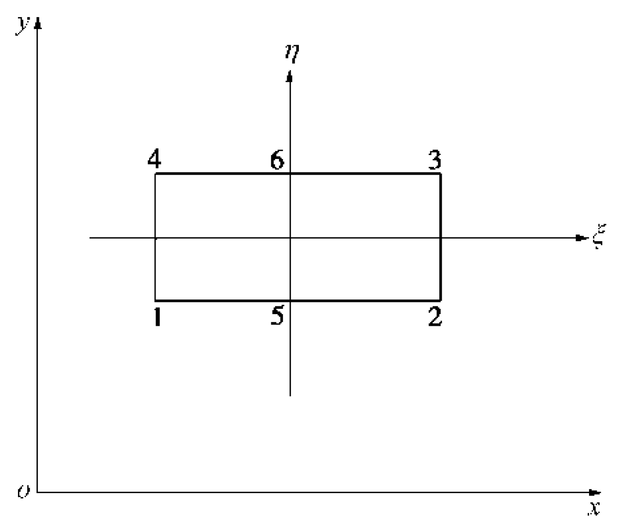
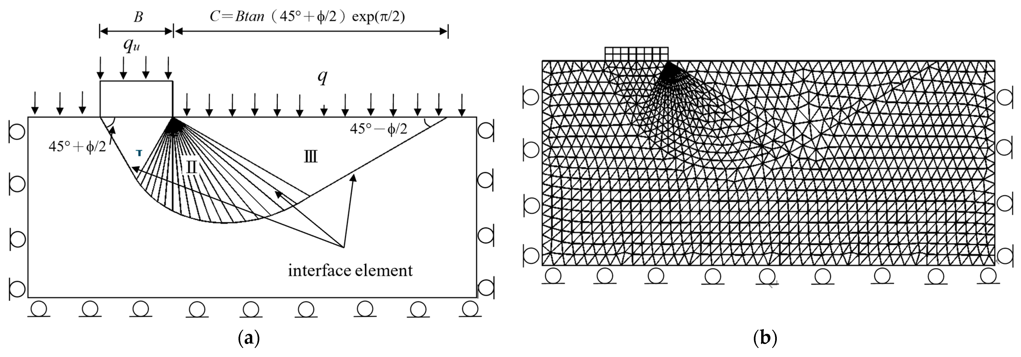
3.2. Establishment of Zero-Thickness Interface Elements in Finite Element Analysis

In the finite element method for solving solid mechanics problems, the analysis of interface elements typically involves three main components: (1) constitutive equations, (2) compatibility equations, and (3) equilibrium equations. These components are used to derive the stiffness matrix that governs the force–displacement relationship, which is obtained through numerical computation. The implementation of multi-segment, zero-thickness interface elements within the finite element analysis framework is described as follows.

(1)

Constitutive law: stress–strain relationship

The stress–strain relationship of general interface elements can be expressed as the relationship between the global and local coordinate systems, including (i) the global coordinate system, $\left\{\sigma \right\}=\left[E\right]\left\{\epsilon \right\}$; (ii) local coordinate system, $\left\{{\sigma }^l\right\}=\left[E^l\right]\left\{{\epsilon }^l\right\}$; and (iii) the relationship between the two coordinate systems, $\left\{\sigma \right\}=\left[R\right]\left\{{\sigma }^l\right\}$ and $\left\{{\epsilon }^l\right\}={\left[R\right]}^T\left\{\epsilon \right\}$. Finally, the result can be expressed as $\left\{\sigma \right\}=\left[R\right]\left[E^l\right]{\left[R\right]}^T\left\{\epsilon \right\}$, where [E] and [E^l] are the stress–strain physical equation matrices of the global and local coordinate systems, respectively. [R] is the relationship transformation matrix between the global coordinate system and the local coordinate system; the superscript l is the interface unit of the local coordinate system.

In the case of a zero-thickness attached interface (within the elastic range), the continuity of the vertical and tangential relative displacements between the two objects must be ensured, and the stress–strain relationship matrix can be expressed as

$$\left[E^l\right]=\left[\begin{array}{ccc}0& 0& 0\\ 0& kE& 0\\ 0& 0& G\end{array}\right]$$

(17)

For simulating the mechanical behavior of imaginary materials, the interface element parameters E and G have no real physical meaning, so the minimum E value of the two contacting solids is generally used as the E value of the imaginary material. As for the Poisson’s ratio ν value, since the interface element has no thickness, it is assumed that ν = 0. If the Mohr–Coulomb friction interface is considered, when there is relative displacement between the two solids, that is, when a complete sliding condition occurs (G = 0), the stress–strain relationship matrix can be expressed as

$$\left[E^l\right]=\left[\begin{array}{ccc}0& 0& 0\\ 0& kE& 0\\ 0& 0& 0\end{array}\right]$$

(18)

(2)

Compatibility: strain–displacement relationship

When considering zero-thickness interface elements in the finite element analysis, soil elements are generally considered to be parametric elements, such as six- or eight-node triangles, T6, or quadrilaterals, Q8. Because there are three nodes on each side of two adjacent soil elements, it can be assumed that the contact surface interface element is a quadrilateral Q6 parametric element, as shown in Figure 4. Assuming x, y are the global coordinate system, ξ, η are the local coordinate system. The relationship between the coordinate systems and the displacement and shape function of each node in the element can be expressed as follows.

$$\left\{\begin{array}{c}u\\ v\end{array}\right\}={\sum }_{k=1}^N{H}_k\left(\xi , \eta \right)\left\{\begin{array}{c}{u}_k\\ v_k\end{array}\right\}$$

(19)

and

$$\left\{\begin{array}{c}x\\ y\end{array}\right\}={\sum }_{k=1}^N{H}_k\left(\xi , \eta \right)\left\{\begin{array}{c}{x}_k\\ y_k\end{array}\right\}$$

(20)

where x_k, y_k are the coordinates on node k. u, v are the node displacements on the element. u_k, v_k are the displacements on node k. N is the element node number. H_k $\left(\xi , \eta \right)$ is the interpolated shape function ($-1\subseteq \xi , \eta \subseteq 1$) on node k.

Assuming that the thickness of the interface element is e, the single-side curve M of nodes 1, 5, and 2 corresponds to the interpolation coordinate system. $\left(\xi , \eta \right)$ and can be expressed as

$$M\left\{\begin{array}{c}x\\ y\end{array}\right\}=\left\{\begin{array}{c}x\left(\xi \right)=g_1\left(\xi \right)x_1+g_2\left(\xi \right)x_2+g_5\left(\xi \right)x_5\\ y\left(\xi \right)=g_1\left(\xi \right)y_1+g_2\left(\xi \right)y_2+g_5\left(\xi \right)y_5\end{array}\right.$$

(21)

where g₁(ξ), g₂(ξ), and g₅(ξ) are all shape functions and can be defined by Lagrange polynomial equations. If (T, N) are vector components on the curve, M, and are perpendicular to each other, then T·N = −1, which can be expressed as

$$N(\xi )=\left\{\begin{array}{c}{\displaystyle \frac{\partial x}{\partial \xi }}={\displaystyle \frac{1}{2}}(-x_1+x_2)+\xi (x_1+x_2-2x_5)\\ -{\displaystyle \frac{\partial y}{\partial \xi }}=-{\displaystyle \frac{1}{2}}(-y_1+y_2)-\xi (y_1+y_2-2y_5)\end{array}\right.$$

(22)

Considering that the interface element is an element with a very small thickness, e, as shown in Figure 4, the coordinates of nodes 2, 1, and 5 corresponding to nodes 3, 4, and 6 can be expressed as

$$\left\{\begin{array}{c}{x}_3\\ y_3\end{array}\right\}=\left\{\begin{array}{c}{x}_2\\ y_2\end{array}\right\}+e{\displaystyle \frac{N(\xi =+1)}{‖N(+1)‖}}$$

(23)

$$\left\{\begin{array}{c}{x}_4\\ y_4\end{array}\right\}=\left\{\begin{array}{c}{x}_1\\ y_1\end{array}\right\}+e{\displaystyle \frac{N(\xi =-1)}{‖N(-1)‖}}$$

(24)

$$\left\{\begin{array}{c}{x}_6\\ y_6\end{array}\right\}=\left\{\begin{array}{c}{x}_5\\ y_5\end{array}\right\}+e{\displaystyle \frac{N(\xi =0)}{‖N\left(0\right)‖}}$$

(25)

where the definition is that e = 10^−nL and L = 0.5 [(x_max − x_min) − (y_max − y_min)]. Since L is a deformable function, to maintain the thickness, e, at a minimum value, the ratio of e/L should be in the order of 10⁻⁴ to 10⁻⁶.

(3)

Equilibrium: Energy conservation equations

Based on the displacement analysis of the finite element method, the element node displacement is used as the unknown number of the problem. This unknown number can be obtained using the node equilibrium equation group and the total potential energy principle. The energy conservation equation can be given as

$${\delta W}_{int}+\delta W_{ext}=0$$

(26)

where δW_int is the internal strain energy; δW_ext is the work performed by the external potential energy. In the range of domain, $\mathsf{\Omega }$, it can also be expressed as

$$\delta W_{int}=-{\int }_{ \Omega }\left(\sigma \right)\left\{\delta \epsilon \right\}d\Omega$$

(27)

According to the displacement–strain relationship, it is expressed in the matrix form as

$$\left\{\epsilon \right\}=\left[B\right]\left\{U^l\right\}$$

(28)

or

$$\left\{\epsilon \right\}=\left[A\right]\left[T\right]\left[L\right]\left\{U^l\right\}$$

(29)

where {U^l} is the displacement of the element in the global coordinate. [B] is the displacement–strain transformation transpose matrix. [A] is the strain–displacement transformation relationship matrix. [L] is the node displacement function. Finally, the stress matrix can be expressed as

$$\left\{\sigma \right\}=\left[E\right]\left\{\epsilon \right\}=\left[R\right]\left[E^l\right]\left[R{]}^T\right\{\epsilon \}$$

(30)

or

$$\left\{\sigma \right\}=\left\{U^l\right\}\left[B{]}^T\right[E]$$

(31)

In addition, according to the strain energy principle, the internal strain energy can be expressed as

$${\delta W}_{int}=-⟨U^l⟩{\int }_{ \Omega }\left[B{]}^T\right[E\left]\right[B\left]\right\{\delta U^l\}d\Omega$$

(32)

or

$${\delta W}_{int}=-⟨U^l⟩\left[K^l\right]\left\{\delta U^l\right\}$$

(33)

where [K^l] is the element stiffness matrix, which can be expressed as

$$\left[K^l\right]={\int }_{ \Omega }\left[B{]}^T\right[E\left]\right[B]d\Omega$$

(34)

In the case of extremely low thickness, it can be expressed as

$$\left[K^l\right]=\int {\int }_{-1}^{+1}\left[B{]}^T\right[E\left]\right[B]\left|\mathit{det}J\right|d\xi d\eta$$

(35)

where J is the Jacobin matrix and $\left|\mathit{det}J\right|$ is the Jacobin determinant.

3.3. Application Principle and Operation Process of Zero-Thickness Interface Elements

In analyzing the mechanical behavior of conventional thickness interface elements, three primary states are typically considered: adhesion, relative displacement (sliding), and separation. Therefore, the finite element calculation process must include the following steps: (1) identifying the contact area at each load increment; (2) distinguishing between the sliding zone, where relative displacement occurs, and the adhesion zone, where no relative displacement is observed; and (3) evaluating whether the interface element stress reaches a failure criterion, leading to either relative displacement or separation during each incremental step. When implementing zero-thickness interface elements in finite element analysis and programming, the procedure must first address the mechanical constraints and deformation behavior at the contact surface, as illustrated in Figure 5.

It can be seen from Figure 5 that a and b represent two contacting objects, and M represents the contact point. When point M is relatively displaced due to an external force, the displacement of its global coordinate system can be given as

$$\begin{array}{c}{x}^{*}=x+\Delta u\\ y^{*}=y+\Delta v\end{array}$$

(36)

where (x*, y*) are the coordinates after displacement. The volume increment of the initial contact volume of the interface element after conversion can be given as

$$d{V}^{*}=\left|\left.\begin{array}{cc}{\displaystyle \frac{\partial x^{*}}{\partial x}}& {\displaystyle \frac{\partial x^{*}}{\partial y}}\\ {\displaystyle \frac{\partial y^{*}}{\partial x}}& {\displaystyle \frac{\partial y^{*}}{\partial y}}\end{array}\right|dxdy\right.$$

(37)

This equation can also be expressed as $d{V}^{*}=\left(\mathit{det}{F}^{*}\right)dV$, where $\mathit{det}{F}^{*}$ is the partial differential of the volume increment. When $\mathit{det}{F}^{*}>0$, it indicates that the two objects are separated and displaced. When $\mathit{det}{F}^{*}=0$, this indicates that the two objects are attached, and when $\mathit{det}{F}^{*}<0$, this indicates that the objects are squeezed and deformed, or relative displacement occurs. Therefore, its displacement can be expressed as

$$\begin{array}{c}{x}_a=x+\alpha \Delta u\\ y_a=y+\alpha \Delta v\end{array}$$

(38)

It can be seen from the above equation that when $\mathit{det}{F}_{\alpha =0}=1>0$, it indicates that no deformation occurs (the initial contact area is equal to the contact area after the force is applied); when $\mathit{det}{F}_{\alpha =1}=\mathit{det}{F}^{*}<0$, it indicates that the two objects produce relative displacement but are not completely separated.

Assume that the external force acting on the interface element, σ_n, is normal stress. When the interface element is in the startup state, the relationship can be given as

$${\sigma }_n={\sigma }_n^0+\Delta {\sigma }_n\ge R_T$$

(39)

where the relative coefficient λ is

$$\lambda ={\displaystyle \frac{R_T-{\sigma }_n^0}{\Delta {\sigma }_n}}$$

(40)

When the finite element analysis is used to calculate with the zero-thickness interface element, the stress is mainly calculated by using relative displacement. Therefore, the principle of virtual work can be applied to simulate the situation where the interface elements cannot withstand shear force when they are in a sliding state. The numerical calculation steps are as follows: (1) Calculate the stiffness matrix of the interface elements [K_i] and [K_i+1], and triangulate the stiffness matrix [K_i]; (2) Calculate $\left[K_i\right]\{\Delta U_i\}=\left\{R_{i-1}\right\}$; (3) Calculate the stress increment vector {Δσ_i} and the displacement increment vector {ΔU_i}; (4) Calculate the force vector {R_i}; and (5) Test the convergence of the equilibrium force.

The numerical calculation process for two-dimensional finite element analysis in this study is divided into three main components: (1) pre-processing, (2) main calculation and analysis, and (3) post-processing.

Pre-processing involves defining the analysis domain and boundary conditions, automatically generating meshes for both block and interface elements, optimizing the matrix structure, and inputting parameters for each module. These parameters include, in sequence, bulk density, Young’s modulus, Poisson’s ratio, cohesion, internal friction angle, and dilation angle. Additional pre-processing steps include specifying boundary constraints, calculating initial stresses based on defined parameters, applying external loads, performing force superposition, conducting convergence iterations, checking for mesh penetration, and ultimately generating a base data file for analysis.

The main calculation and analysis phase begins with the input of execution commands and the loading of the data file produced during pre-processing. During this phase, the program reads the element parameters for each element group, the global coordinates of each node, the material properties of each module, and the degrees of freedom and load conditions at each node. The results are then sent to an output data file.

Post-processing uses the output data to generate visual representations of the analysis results. These include stress variation diagrams, progressive failure diagrams, mesh deformation plots, equivalent displacement maps, and displacement field diagrams. From these results, the stage at which failure occurs in the load increment process is identified, allowing for the calculation of the minimum upper-bound limit of the soil’s ultimate bearing capacity.

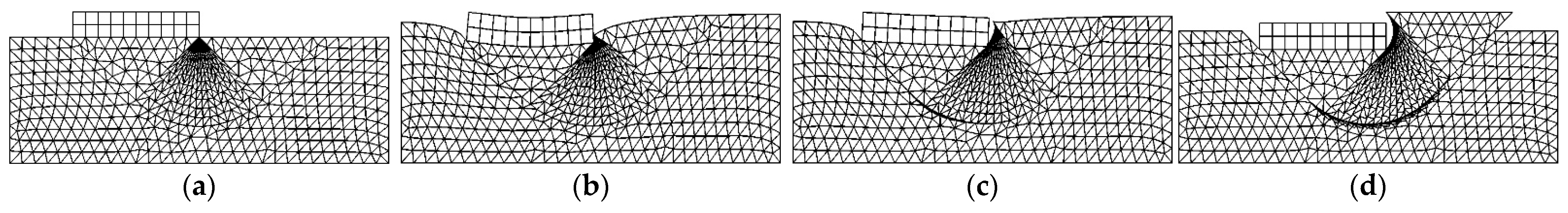
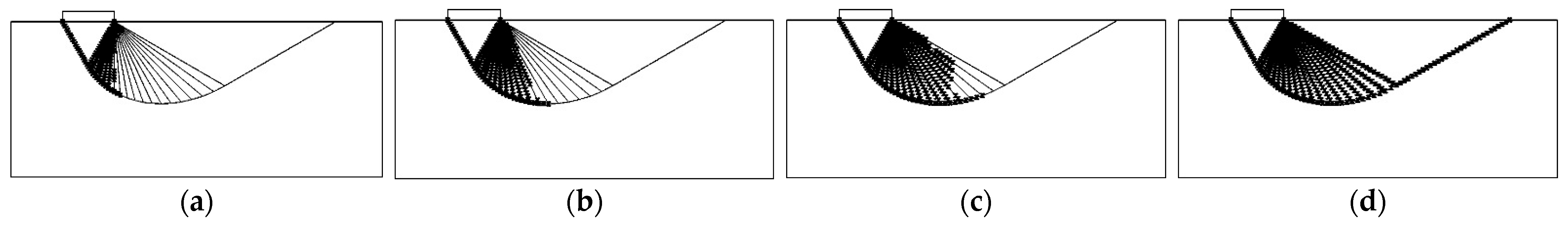
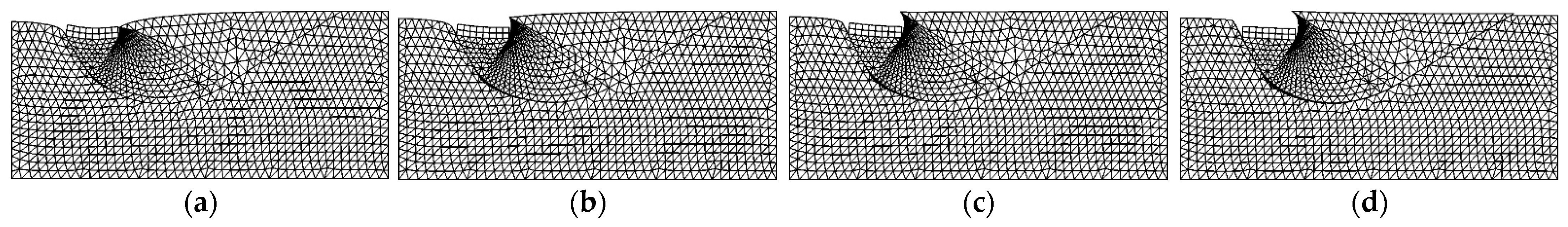
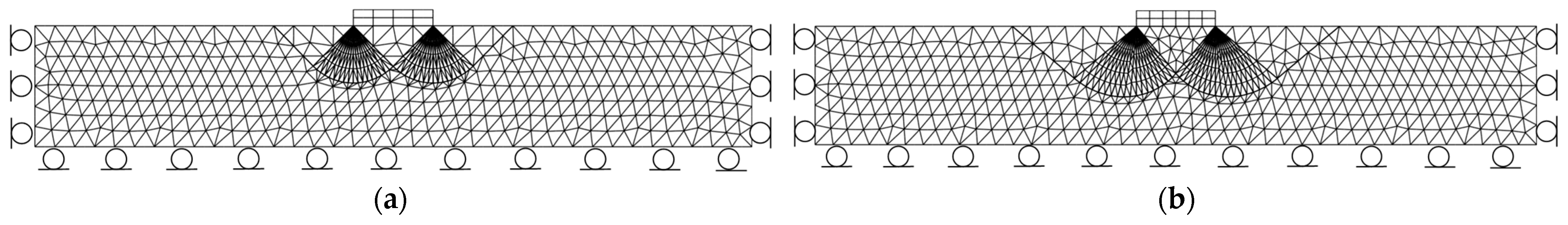
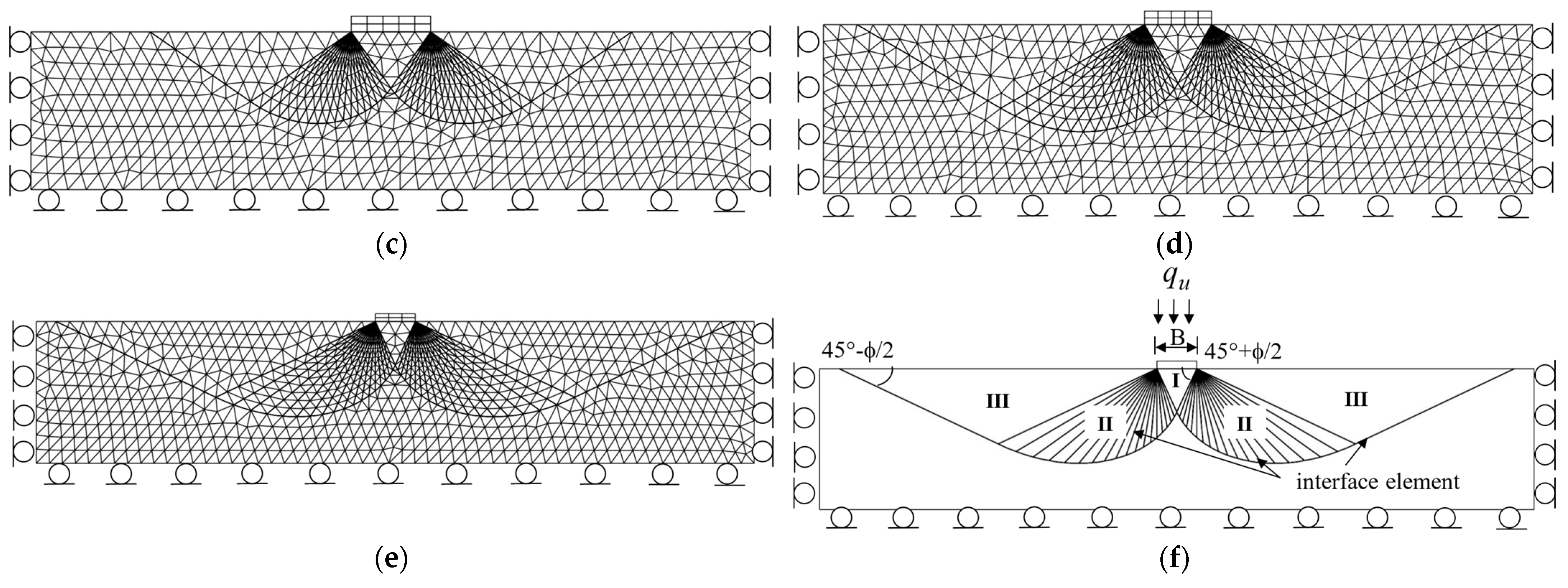
4. Verification Between Numerical and Analytical Results

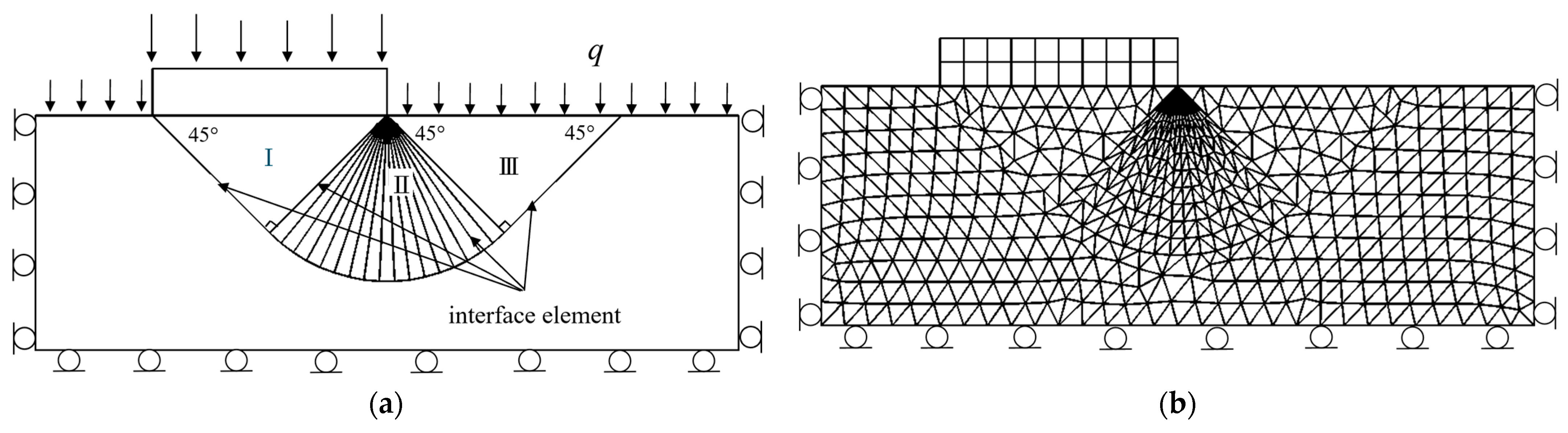
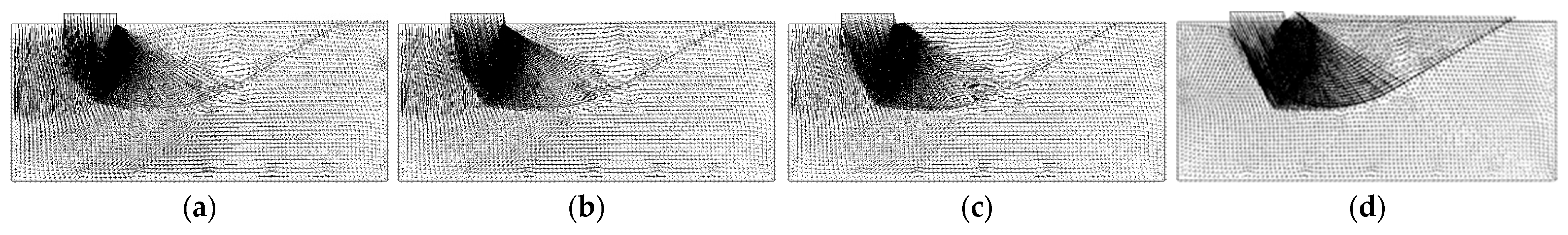
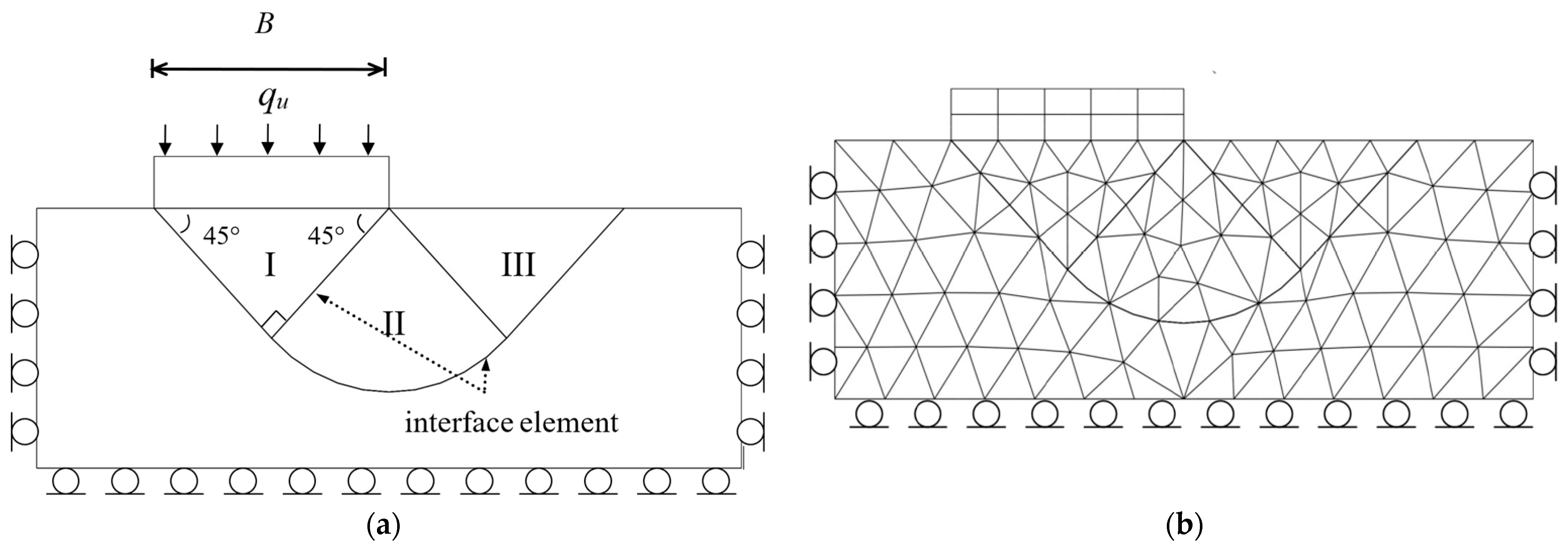
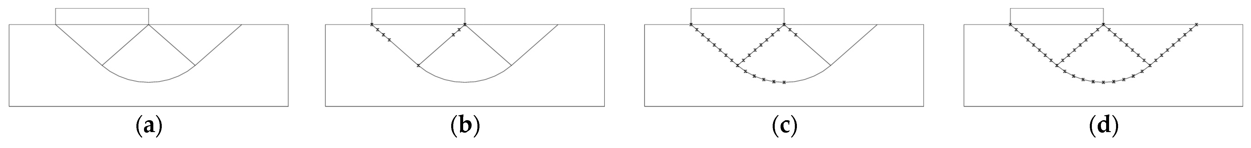
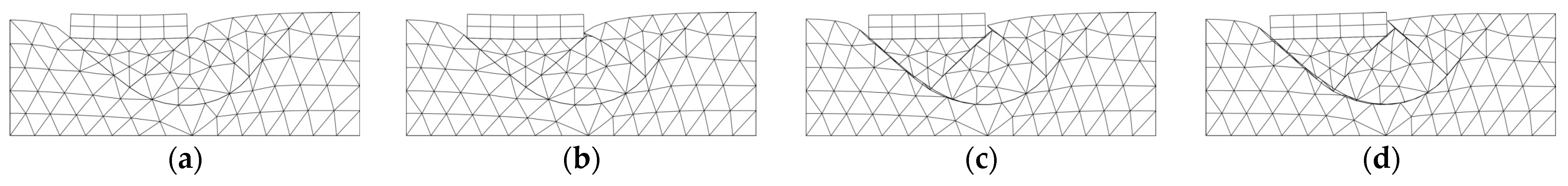
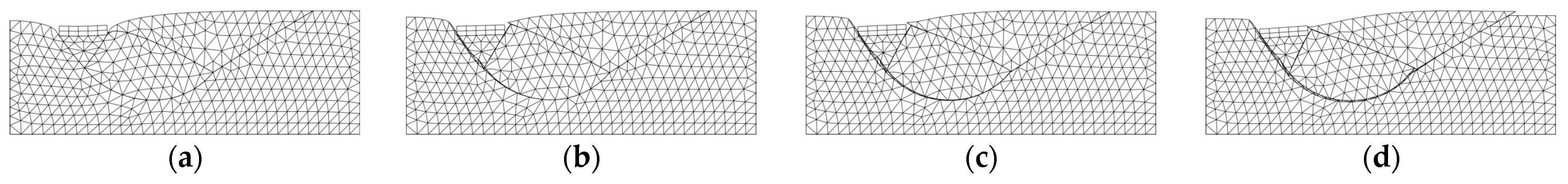
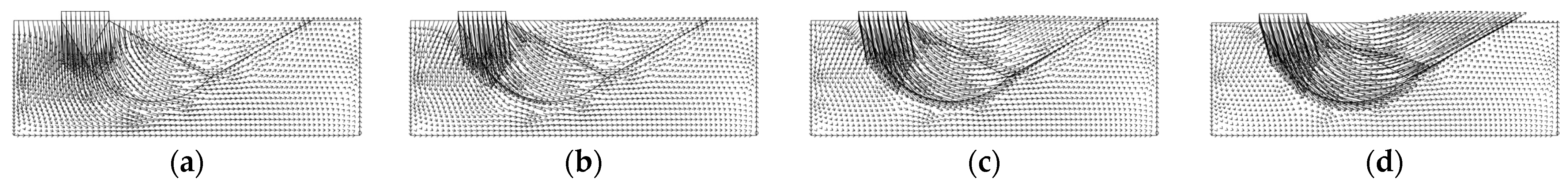
4.1. Analysis of the Ultimate Bearing Capacity of Shallow Foundations in Cohesive Soils

To analyze the soil failure mechanism induced by shallow foundation loading, this study investigates the relationship between soil cohesion and the resulting failure mechanism and calculates the ultimate bearing capacity of cohesive soil. In the finite element analysis, the assumed failure mechanism is a composite sliding surface consisting of triangular and fan-shaped zones, as illustrated in Figure 1. Based on this assumed mechanism, a simulation of soil failure under a shallow foundation load is conducted, and the ultimate bearing capacity is determined accordingly. For cohesive soils, the failure mechanism is characterized by a sliding surface comprising two triangular zones and a central fan-shaped zone, referred to as the active zone (I), the transition zone (II), and the passive zone (III), as depicted in Figure 6a. The corresponding finite element mesh for this configuration is shown in Figure 6b. The ultimate bearing capacity of the shallow foundation under these conditions can be analytically determined using Equation (8).

To better understand the sliding failure behavior within the fan-shaped zone and to evaluate the accuracy of different minimum upper-bound estimates, this study subdivided the sector into multiple slices and employed a multi-segment, zero-thickness interface element for simulation. Convergence analysis showed that the error between the numerical results and the upper-bound solution from the limit analysis was minimized when the sector was divided into 30 slices, corresponding to an internal angle of 3° for each slice within the 90° fan-shaped zone. To streamline the mesh generation process while maintaining sufficient accuracy, this study adopts a simplified configuration of 18 slices, where each internal angle is 5°. The analysis employs a multi-segment, zero-thickness interface element formulation, and the corresponding finite element mesh diagram is illustrated in Figure 6b.

In the finite element analysis, the shallow foundation is assumed to be placed in a semi-infinite space, with two triangular zones and a single fan-shaped transition zone forming the failure mechanism The failure is modeled as five sliding surfaces, two triangles, and one fan-shaped group. For each section of the zero-thickness interface, the Mohr–Coulomb parameters are set with a friction angle (φ) of 0 and undrained shear strength (c_u), with soil cohesion normalized for the simulation. The simulation results, shown in

Table 1. Comparison of the results obtained by numerical calculations and analytical solutions.

Analysis Case	Failure Mechanism	Upper-Bound Limit of the Ultimate Bearing Capacity of Shallow Foundations, qu
		Atkinson (1980) [16]	F.E.M.
Cohesive soil (q = 0, c = cu, φ = 0)	Two triangular and fan-shaped groups	(2 + π) cu	5.14 cu
C-phi soil (q, c = 0, φ = 30°)	Two triangular and logarithmic spirals	1.84 q	1.84 q

, indicate that the error between the numerical analysis and the upper-bound value of the ultimate bearing capacity proposed by Atkinson (1981) [16] is only 0.55% (using 18 sector slices for analysis). Based on Equation (8), the ratio of the ultimate bearing capacity to the undrained shear strength of the shallow foundation is calculated as q_u/c_u = 5.14. At this load level, all points on the sliding surface are predicted to reach complete sliding failure, as illustrated in Figure 7. The failure process follows a progressive pattern from left to right. Initially, the triangular active zone (I) undergoes sliding failure. As the stress redistribution progresses, failure spreads into the fan-shaped transition zone (II) and eventually to the triangular passive zone (III). When the incremental accumulation reaches completion, the entire sliding surface has undergone total failure.

Figure 7 illustrates the progressive failure diagrams corresponding to different stages of loading: (a) 10%, (b) 40%, (c) 70%, and (d) 100% of the applied load. As loading increments are applied, sliding failure progressively develops along the predefined sliding surface, and the foundation undergoes increasing settlement. By the final stage of loading (100%), all points along the sliding surface, comprising the two triangular zones and the central fan-shaped zone, have entered a plastic failure state. This progressive failure behavior is also reflected in the overall displacement and deformation diagrams at each increment. During this process, the triangular passive zone (zone III) exhibits noticeable plastic volumetric expansion. The displacement trends are further visualized in the form of displacement fields (Figure 8) and corresponding finite element meshes (Figure 9), clearly showing that the deformation aligns with the sliding failure surface as the load reaches its ultimate value.

4.2. Analysis of the Ultimate Bearing Capacity of Shallow Foundations in C-Phi Soils

The simulation of the soil failure mechanism induced by shallow foundation loading primarily involves two components: the assumed failure mechanism and the calculation of the ultimate bearing capacity. As illustrated in Figure 2a, the failure mechanism is composed of two triangular zones, the active zone (I) and the passive zone (III), connected by multiple slip surfaces that form a logarithmic spiral group, representing the transition zone (II). This composite mechanism captures the progressive nature of soil failure under loading. In addition, the corresponding velocity field associated with this assumed mechanism is depicted in Figure 2b, providing an insight into the soil movement and deformation patterns during failure.

The schematic representation of the distribution of multi-segment zero-thickness interface elements used for analyzing the ultimate bearing capacity of shallow foundations is shown in Figure 10a, while the corresponding finite element mesh is depicted in Figure 10b. The results from the finite element analysis indicate that all points along the predefined slip surface eventually reach complete sliding failure. Moreover, the numerical results closely align with those obtained from upper-bound limit analysis. For soil with an internal friction angle of 30°, the computed ratio of ultimate bearing capacity to cohesion, q_u/c_u, is 1.84. A detailed comparison of these results is provided in Table 1.

As illustrated in Figure 11, the numerical results under varying loading percentages, 10%, 40%, 70%, and 100%, demonstrate that failure along the slip surface progresses incrementally from top to bottom and from left to right. Specifically, as stress redistributes during loading, failure initiates in the active zone (zone I), propagates through the spiral transition zone (zone II), and finally ruptures along the slip surface in the passive zone (zone III). Upon completion of the incremental loading, as shown in Figure 11d, all points on the slip surface experience full sliding failure. These numerical results closely align with the minimum upper-bound solution derived from the limit analysis, confirming that the shallow foundation induces a progressive failure mechanism in the surrounding soil under applied load. In addition, Figure 12 depicts the deformation and rupture of the finite element mesh along the slip surface, while Figure 13 illustrates the trend of the velocity field throughout the failure process. The results, as presented in Table 1, indicate that the numerical calculations are in close agreement with the upper-bound solution for the ultimate bearing capacity of shallow foundations proposed by Atkinson (1981) [16].

Although the method is based on plastic collapse and does not explicitly simulate elastic deformation, we varied the stiffness ratio from 100 to 1000 to evaluate any indirect influence on interface behavior. The bearing capacity predictions remained stable across this range, and load–displacement convergence behavior was unaffected. To assess the numerical stability of the method, we varied the mesh density in non-transition zones by scaling the base mesh size. It indicates that the solution is largely mesh-independent outside the slip zone, due to the structured nature of the predefined failure mechanism.

5. Discussion

In this study, multi-segment zero-thickness interface elements based on the Mohr–Coulomb failure criterion are employed to simulate the progressive failure of the proposed failure mechanisms. The analysis is conducted under two soil conditions: cohesive soil and C-phi soils, in which cohesion remains constant while the internal friction angle varies at 10°, 20°, 30°, and 40°. This study investigates how various influencing factors, such as the number of discretized blocks in the transition zone of the failure mechanism and the bearing capacity factors, N_c and N_q, affect the ultimate bearing capacity of shallow foundations.

To gain a deeper insight into the sliding failure behavior of the transition zone (zone II) in both cohesive and C-phi soils, particular emphasis is placed on analyzing the effect of varying the number of discretized segments within this zone. The results of this analysis are discussed in the following sections.

5.1. Cohesive Soils

Assume a shallow foundation located in a semi-infinite space. The failure mechanism of cohesive soil directly below the foundation consists of a triangular active zone (I), a fan-shaped zone (II), and a triangular passive zone (III) on its right side, as shown in Figure 6a. In this study, the fan-shaped zone is subdivided into n blocks (including n = 1, 2, 3, 5, 6, 9, 10, 15, 18, and 30). Figure 14 especially shows the case study with block number n = 1. The Mohr–Coulomb interface parameters at each stage are c = c_u and ϕ = 0°, and the numerical analysis results are shown in

Table 2. Influence of block number in the transition zone of the failure mechanism of cohesive soils.

Block Number (n)	Ultimate Bearing Capacity (F.E.M.), qu/cu	Error Percentage * (%)	Calculation Time **
1	6.51	26.65	39.18 s
2	5.74	11.67	37.88 s
3	5.50	7.00	53.52 s
5	5.33	3.70	1 min 15.77 s
6	5.29	2.92	2 min 0.04 s
8	5.25	2.14	1 min 28.61 s
9	5.23	1.75	2 min 57.73 s
10	5.22	1.56	4 min 37.85 s
15	5.18	0.78	15 min 43.50 s
18	5.15	0.19	19 min 52.12 s
30	5.14	0.00	52 min 44.78 s

* $Error percentage\left(\%\right)={\displaystyle \frac{\mathrm{F}.\mathrm{E}.\mathrm{M}.-\mathrm{E}\mathrm{q}\mathrm{u}\mathrm{a}\mathrm{t}\mathrm{i}\mathrm{o}\mathrm{n}\left(9\right)}{\mathrm{E}\mathrm{q}\mathrm{u}\mathrm{a}\mathrm{t}\mathrm{i}\mathrm{o}\mathrm{n}\left(9\right)}}100\%$. ** Calculation time via Sun Blade 100 (workstation).

. This table demonstrates that increasing the number of subdivisions, n, in the transition zone significantly reduces the error between the numerical results and the analytical solution. When the transition zone is divided into 18 blocks, the error margin decreases to approximately 0.19%, indicating that the finite element analysis achieves efficient convergence at this level of discretization. These findings suggest that appropriately refining the transition zone enhances the compatibility of displacement between rotational and sliding motions, as shown in Figure 15. Based on the analysis, it is recommended to subdivide the transition zone using a segmentation angle of 5°, which corresponds to 18 blocks within the 90° fan-shaped sector, to achieve optimal accuracy and computational efficiency.

Figure 6, Figure 7, Figure 8 and Figure 9 illustrate the simulation and analysis results at various loading stages when the transition zone is subdivided into 18 blocks. These results highlight the progressive failure behavior and effective convergence achieved through finer discretization. In contrast, Figure 16, Figure 17 and Figure 18 present the outcomes when the transition zone is modeled as a single block, revealing noticeable differences in deformation patterns, stress distribution, and failure progression compared to the multi-block configuration. Especially in the ultimate bearing capacity value, a large percentage error is shown.

5.2. C-Phi Soils

This section examines the influence of the block number within the C-phi soil transition zone on the bearing capacity factors N_c and N_q. For the C-phi soil conditions described in Section 4.2 and illustrated in Figure 2a, the shallow foundation failure mechanism is assumed to consist of two triangular zones, namely, the active zone (zone I) and the passive zone (zone III), along with a transition zone (zone II) characterized by multiple slip surfaces forming a spiral mechanism. The block number refers to the discretization used to model the spiral slip surface within the transition zone, and it plays a significant role in determining the accuracy of the computed bearing capacity factors.

In this study, the spiral zone is subdivided into n blocks (including n = 1, 2, 3, 5, 6, 9, 10, 15, 18, and 30). Figure 19 especially shows the case study with block number n = 1. The Mohr–Coulomb interface parameters at each stage are c = c_u and φ = 30°, and the numerical analysis results are shown in

Table 3. Influence of block number in the transition zone of the failure mechanism of C-phi soils.

Block Number (n)	Ultimate Bearing Capacity (F.E.M.), qu/cu	Error Percentage * (%)	Calculation Time **
1	22.13	20.27	1 h 23 min
2	21.64	17.61	1 h 17 min
3	21.16	15	1 h 20 min
5	20.64	12.17	1 h 15 min
6	20.23	9.95	1 h 25 min
8	19.35	5.16	1 h 14 min
9	18.56	0.87	1 h 18 min
10	18.48	0.43	1 h 27 min
15	18.44	0.22	2 h 25 min
18	18.42	0.11	2 h 39 min
30	18.41	0.05	6 h 17 min

* $Error percentage\left(\%\right)={\displaystyle \frac{\mathrm{F}.\mathrm{E}.\mathrm{M}.-\mathrm{E}\mathrm{q}\mathrm{u}\mathrm{a}\mathrm{t}\mathrm{i}\mathrm{o}\mathrm{n}\left(41\right)}{\mathrm{E}\mathrm{q}\mathrm{u}\mathrm{a}\mathrm{t}\mathrm{i}\mathrm{o}\mathrm{n}\left(41\right)}}100\%$. ** Calculation time via Sun Blade 100 (workstation).

and

Table 4. Influence of block number in the transition zone of the failure mechanism of C-phi soils.

Block Number (n)	Ultimate Bearing Capacity (F.E.M.), qu/cu	Error Percentage * (%)
1	36.53	21.20
2	35.75	18.61
3	34.92	15.86
5	34.26	13.67
6	33.35	10.65
8	31.84	5.64
9	30.50	1.19
10	30.27	0.43
15	30.21	0.23
18	30.17	0.1
30	30.15	0.03

* $Error percentage\left(\%\right)={\displaystyle \frac{\mathrm{F}.\mathrm{E}.\mathrm{M}.-\mathrm{E}\mathrm{q}\mathrm{u}\mathrm{a}\mathrm{t}\mathrm{i}\mathrm{o}\mathrm{n}\left(42\right)}{\mathrm{E}\mathrm{q}\mathrm{u}\mathrm{a}\mathrm{t}\mathrm{i}\mathrm{o}\mathrm{n}\left(42\right)}}100\%.$

. According to the analytical solutions of N_q and N_c proposed by Vesic (1973) [4], it can be given as follows

$$N_q={\mathit{tan}}^2({\displaystyle \frac{\pi }{4}}+{\displaystyle \frac{\phi }{2}})e^{\pi \mathit{tan}\phi }$$

(41)

$$N_c=\left(N_q-1\right)\mathit{cot}\phi$$

(42)

Table 3 and Table 4 present the ultimate bearing capacity values calculated using c = cu and φ = 30°. Since the analysis is conducted in terms of the undrained shear strength c_u, the resulting ultimate bearing capacity is dimensionless. Under these conditions, the calculated bearing capacity factors by the equations above are N_q = 18.40 and N_c = 30.14. Figure 10, Figure 11, Figure 12 and Figure 13 illustrate the simulation and analysis results for each loading stage when the transition zone is discretized into 18 blocks. For comparison, Figure 19, Figure 20, Figure 21 and Figure 22 show the results when the transition zone is modeled as a single block, highlighting the differences in the failure mechanism and corresponding bearing capacity response.

As shown in Figure 23, the 18-block model provides a more refined and realistic representation of soil behavior under shallow foundation loading, leading to more accurate bearing capacity estimates. The 1-block model, while simpler, sacrifices fidelity and may misrepresent key aspects of the failure mechanism.

Although traditional upper-bound approaches rely on rigid-body mechanisms, the use of deformable finite elements combined with zero-thickness interfaces enables the simulation of progressive failure and stress redistribution, especially in transition zones. A comparative analysis (presented in Table 2, Table 3 and Table 4) shows that deformation effects, though small in certain idealized cases, become significant in complex geometries or for layered soils, justifying the adoption of a deformable FE framework.

Mesh optimization in this study refers to the partitioning strategy applied to the transition zone. The zone is discretized into 18 blocks with varying dimensions to balance computational efficiency and accuracy. While not automatic in the sense of adaptive remeshing, this structured refinement minimizes numerical diffusion and improves convergence, as demonstrated in Figure 6 and Figure 10.

While the method relies on predefined failure surfaces, it offers engineers a practical and computationally efficient tool for problems where standard mechanism shapes (e.g., circular, log-spiral) are a reasonable assumption. Unlike optimization-based FELA techniques, the present method allows a rapid evaluation with a clear physical interpretation, making it well suited for preliminary design and parametric studies.

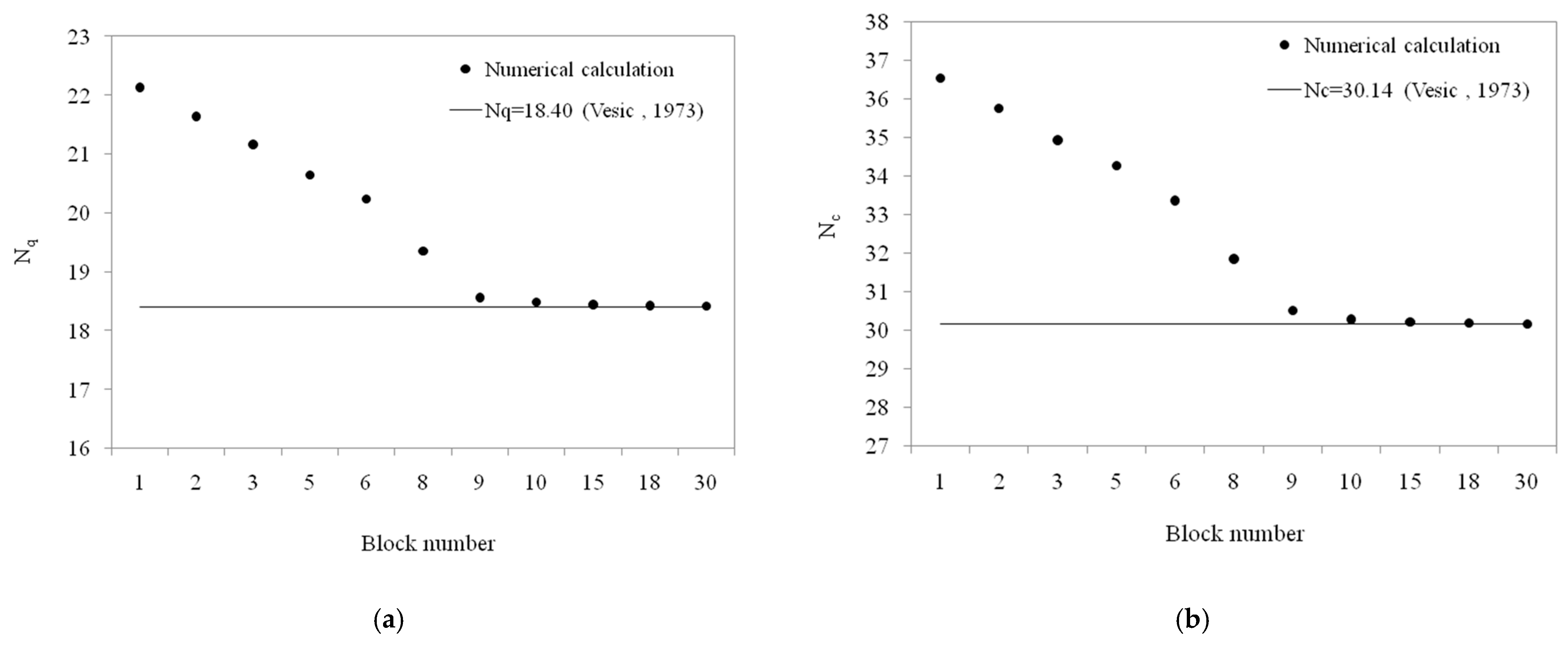
5.3. Discussion of the Bearing Capacity Factors N_q and N_c

A shallow foundation was considered in a semi-infinite soil medium to investigate the effects of varying internal friction angles (φ = 0°, 10°, 20°, 30°, and 40°) on the bearing capacity factors Nc and Nq, as well as the progressive failure mechanisms. The assumed failure mechanism initiates with the collapse of the triangular active zone located directly beneath the foundation. As loading increases, stress accumulation leads to progressive failure within the transition zone, where slip surfaces sequentially fail. Finally, complete sliding failure occurs in the triangular passive zone. Five distinct failure mechanisms, corresponding to the five different friction angles, are illustrated in Figure 24, Figure 25, Figure 26 and Figure 27. In the analysis, the logarithmic spiral region of the transition zone is discretized into 18 blocks, each spanning an angle of 5°. The sliding surfaces are modeled using multi-segment zero-thickness interface elements, enabling deformation to occur along the tangential direction of the slip surface.

The numerical results for the bearing capacity factors N_q and N_c, as presented in

Table 5. Comparison between numerical and analytical solutions of the bearing capacity factor N_q.

Friction Angle, φ (°)	Vesic (1973) [4], Nq	F.E.M.	Error Percentage * (%)
10	2.47	2.53	2.43
20	6.40	6.44	0.63
30	18.40	18.48	0.43
40	64.20	64.28	0.12

* $Error percentage\left(\%\right)={\displaystyle \frac{\mathrm{F}.\mathrm{E}.\mathrm{M}.-\mathrm{E}\mathrm{q}\mathrm{u}\mathrm{a}\mathrm{t}\mathrm{i}\mathrm{o}\mathrm{n}\left(41\right)}{\mathrm{E}\mathrm{q}\mathrm{u}\mathrm{a}\mathrm{t}\mathrm{i}\mathrm{o}\mathrm{n}\left(41\right)}}100\%.$

and

Table 6. Comparison between numerical and analytical solutions of bearing capacity factor N_c.

Friction Angle, φ (°)	Vesic (1973) [4], Nc	F.E.M.	Error Percentage * (%)
0	5.14	5.15	0.19
10	8.35	8.39	0.48
20	14.83	14.86	0.20
30	30.14	30.16	0.07
40	75.31	75.34	0.04

* $Error percentage\left(\%\right)={\displaystyle \frac{\mathrm{F}.\mathrm{E}.\mathrm{M}.-\mathrm{E}\mathrm{q}\mathrm{u}\mathrm{a}\mathrm{t}\mathrm{i}\mathrm{o}\mathrm{n}\left(42\right)}{\mathrm{E}\mathrm{q}\mathrm{u}\mathrm{a}\mathrm{t}\mathrm{i}\mathrm{o}\mathrm{n}\left(42\right)}}100\%.$

, respectively, obtained through finite element analysis, show an agreement with the theoretical predictions proposed by Vesic (1973) [4].

The numerical results for the bearing capacity factors N_q and N_c, shown in Table 5 and Table 6, demonstrate an agreement with the theoretical values proposed by Vesic (1973) [4]. For N_q, the maximum error percentage across friction angles φ = 10° to 40° is only 2.43%, observed at ϕ = 10°, while the minimum error is just 0.12% at φ = 40°. Similarly, for N_c, the error remains very small across all friction angles, with a maximum of 0.48% at φ = 10° and a minimum of 0.04% at φ = 40°. These results confirm the accuracy and reliability of the finite element modeling approach used in this study.

For the limitations and future extensions, while the proposed method demonstrates high accuracy and efficiency for two-dimensional, homogeneous soil conditions, certain limitations must be acknowledged. First, the current implementation assumes predefined failure mechanisms in a 2D plane–strain context, which may not directly extend to 3D problems where spatial failure surfaces are more complex and may involve out-of-plane effects. Adapting the framework to 3D would require either an analytical extension of the failure geometry or integration with automated mechanism detection algorithms. Second, the model assumes homogeneous and isotropic soil properties; extending it to layered or anisotropic soils would necessitate assigning spatially variable strength parameters and refining the energy dissipation formulation accordingly. Finally, the method may not be suitable in scenarios involving highly compressible materials, strain-softening behavior, or footing–soil interfaces with significant roughness. In such cases, incorporating compressibility corrections, softening laws, or interface roughness factors would be necessary to maintain predictive accuracy.

6. Conclusions

In this study, a self-developed finite element program was employed to evaluate the upper-bound ultimate bearing capacity of shallow foundations in cohesive and C-phi soils. The method incorporates multi-segment zero-thickness interface elements to simulate complex failure mechanisms, based on the Mohr–Coulomb failure criterion, within a semi-infinite soil domain. Key findings include:

(1)

Failure Mechanisms: For purely cohesive soils, the optimal failure mechanism comprises two triangular zones and a circular sector. For C-phi soils, it consists of two triangular zones and a logarithmic spiral sector.

(2)

Verification: Numerical results for both soil types show an excellent agreement with the upper-bound solutions by Atkinson (1981) [16], validating the modeling approach.

(3)

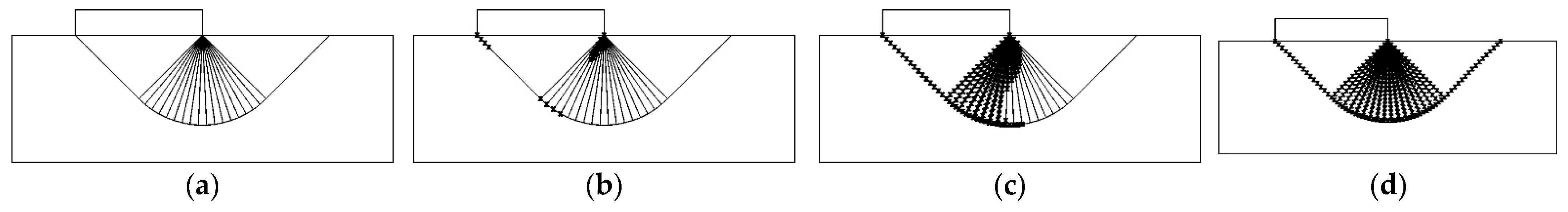
Transition Zone Accuracy: When the transition zone is discretized into 18 blocks, the computed bearing capacity factors closely match Vesic’s (1973) [4] theoretical values, with errors ranging from 0.1% to 0.19%.

(4)

Frictional Soils: For friction angles between 10° and 40°, the computed N_c and N_q values deviate by only 0.04–0.19% and 0.12–2.43%, respectively, from analytical solutions.

The proposed method, while based on assumed mechanism geometry, provides an efficient and accurate tool for evaluating foundation behavior when engineering judgment suggests plausible failure configurations. Unlike discontinuity layout optimization or adaptive limit analysis, our approach emphasizes computational efficiency and transparency in the failure mechanism, which is advantageous for practical design contexts. Nonetheless, we acknowledge that extending the framework to include automatic mechanism detection is a valuable direction for future work.

The primary contribution of this study is the formulation of a structured finite element model using multi-segment zero-thickness interface elements in the transition zone, enabling the high-precision evaluation of upper-bound capacity with minimal deviation from classical solutions. This method achieves excellent agreement (errors < 0.2%) with benchmark solutions while remaining computationally lightweight, offering an efficient alternative to full optimization-based limit analysis.

References

1. De Fazio, N.; Placidi, L.; Tomassi, A.; Fraddosio, A.; Castellano, A.; Paparella, N. Different mechanical models for the study of ultrasonic wave dispersion for mechanical characterization of construction materials. Int. J. Solids Struct. 2025, 315, 113352. [Google Scholar] [CrossRef]
2. Terzaghi, K. Theoretical Soil Mechanics; Wiley: New York, NY, USA, 1943. [Google Scholar]
3. Meyerhof, G.G. The ultimate bearing capacity of foundations. Geotechnique 1951, 2, 301–332. [Google Scholar] [CrossRef]
4. Vesic, A.S. Analysis of ultimate loads of shallow foundations. J. Soil Mech. Found. Div. 1973, 99, 45–73. [Google Scholar] [CrossRef]
5. Silvestri, V. A Limit equilibrium solution for bearing capacity of strip foundations on sand. Can. Geotech. J. 2003, 40, 351–361. [Google Scholar] [CrossRef]
6. Bolton, M.D.; Lau, C.K. Vertical bearing capacity factors for circular and footing foundations on Mohr-Coulomb soil. Can. Geotech. J. 1993, 30, 1024–1033. [Google Scholar] [CrossRef]
7. Sun, H.; Zhao, X.H.; Lo, K.W. Influence of anisotropic damage on ultimate load of plane strain problems for foundation. Comput. Geotech. 2003, 30, 41–60. [Google Scholar] [CrossRef]
8. Zheng, H.; Tham, L.G.; Liu, D. On two definitions of the factor of safety commonly used in the finite element slope stability analysis. Comput. Geotech. 2006, 33, 188–195. [Google Scholar] [CrossRef]
9. Soubra, A.H. Upper-bound solutions for bearing capacity of foundations. J. Geotech. Geoenviron. Eng. 1999, 125, 59–68. [Google Scholar] [CrossRef]
10. Michalowski, R.L. An estimate of the influence of soil weight on bearing capacity using limit analysis. Soils Found. 1997, 37, 57–64. [Google Scholar] [CrossRef]
11. Sloan, S.W. Upper bound limit analysis using finite elements and linear programming. Int. J. Numer. Anal. Methods Geomech. 1989, 13, 263–282. [Google Scholar] [CrossRef]
12. Sloan, S.W.; Kleeman, P.W. Upper bound limit analysis using discontinuous velocity fields. Comput. Methods Appl. Mech. Eng. 1995, 127, 293–314. [Google Scholar] [CrossRef]
13. Zhu, D.Y.; Lee, C.F.; Jiang, H.D. A numerical study of the bearing capacity factor Nγ. Can. Geotech. J. 2001, 38, 1090–1096. [Google Scholar] [CrossRef]
14. Griffiths, D.V. Computation of bearing capacity factors using finite elements. Geotechnique 1982, 32, 195–202. [Google Scholar] [CrossRef]
15. Ugai, K.; Leshchinsky, D. Three-dimensional limit equilibrium and finite element analyses: A comparison of results. Soils Found. 1995, 35, 1–7. [Google Scholar] [CrossRef]
16. Atkinson, J.H. Foundations and Slopes: An Introduction to Applications of Critical State Soil Mechanics; John Wiley & Sons: New York, NY, USA, 1981. [Google Scholar]
17. Chen, W.F. Limit Analysis and Soil Plasticity; Elsevier: Amsterdam, The Netherlands, 1975. [Google Scholar]
18. Cheng, W.F.; Liu, X.L. Limit Analysis in Soil Mechanics; Elsevier: London, UK, 1990. [Google Scholar]
19. Salençon, J. Handbook of Limit Analysis; Wiley: Hoboken, NJ, USA, 2002. [Google Scholar]
20. Sloan, S.W. Lower bound limit analysis using finite elements and linear programming. Int. J. Numer. Anal. Methods Geomech. 1988, 12, 61–77. [Google Scholar] [CrossRef]
21. Lyamin, A.V.; Sloan, S.W. Upper bound limit analysis using finite elements and linear programming. Int. J. Numer. Anal. Methods Geomech. 2002, 26, 181–216. [Google Scholar] [CrossRef]
22. Izadi, A.; Nalkiashari, L.A.; Payan, M.; Chenari, R.J. Bearing capacity of shallow strip foundations on reinforced soil subjected to combined loading using upper bound theorem of finite element limit analysis and second-order cone programming. Comput. Geotech. 2023, 160, 105550. [Google Scholar] [CrossRef]
23. Firouzeh, S.H.; Shirmohammadi, S.; Zanganeh Ranjbar, P.; Payan, M.; Jamsawang, P.; Keawsawasvong, S. Upper bound finite element limit analysis of the response of shallow foundations subjected to dip-slip reverse fault rupture outcrop. Transp. Infrastruct. Geotechnol. 2024, 11, 3256–3292. [Google Scholar] [CrossRef]
24. Jin, L.X.; Qin, T.; Liu, P.T. Upper bound solution analysis of the ultimate bearing capacity of two-layered strip foundation based on improved radial movement optimization. Appl. Sci. 2023, 13, 7299. [Google Scholar] [CrossRef]
25. Krabbenhøft, K.; Lyamin, A.V.; Sloan, S.W. Formulation and solution of some plasticity problems as conic programs. Int. J. Solids Struct. 2007, 44, 1533–1549. [Google Scholar] [CrossRef]
26. Makrodimopoulos, A.; Martin, C.M. Upper bound limit analysis using simplex strain elements and second-order cone programming. Int. J. Numer. Anal. Methods Geomech. 2006, 30, 681–701. [Google Scholar] [CrossRef]
27. Goodman, R.E.; Taylor, R.L.; Brekke, T.L. A model for the mechanics of jointed rock. J. Soil Mech. Found. Div. 1968, 94, 637–659. [Google Scholar] [CrossRef]
28. Day, R.A.; Potts, D.M. Zero thickness interface elements—Numerical stability and application. Int. J. Numer. Anal. Methods Geomech. 1994, 18, 689–708. [Google Scholar] [CrossRef]
29. Smith, C.; Gilbert, M. Application of discontinuity layout optimization to plane plasticity problems. Proc. Math. Phys. Eng. Sci. 2007, 463, 2461–2484. [Google Scholar] [CrossRef]
30. He, L.W.; Schiantella, M.; Gilbert, M.; Smith, C. A Python script for discontinuity layout optimization. Struct. Multidisc. Optim. 2023, 66, 152. [Google Scholar] [CrossRef]
31. Milani, G.; Lourenço, P.B. A discontinuous quasi-upper bound limit analysis approach with sequential linear programming mesh adaptation. Int. J. Mech. Sci. 2009, 51, 89–104. [Google Scholar] [CrossRef]
32. Desai, C.S.; Zaman, M.M.; Lightner, J.G.; Siriwardane, H.J. Interface element for joint and crack modeling. Int. J. Numer. Anal. Methods Geomech. 1984, 8, 19–43. [Google Scholar] [CrossRef]
33. Sharma, K.G.; Desai, C.S. Analysis and implementation of thin-layer element for interface and joints. J. Eng. Mech. 1992, 118, 2442–2462. [Google Scholar] [CrossRef]
34. Potts, D.M.; Zdravković, L. Finite Element Analysis in Geotechnical Engineering: Theory; Thomas Telford: London, UK, 1999. [Google Scholar]
35. ABAQUS Documentation. User’s Manual for Cohesive Elements and Contact Interactions, 2024, Dassault Systèmes. Available online: http://130.149.89.49:2080/v2016/pdf_books/CAE.pdf (accessed on 3 July 2025).
36. Smith, I.M.; Griffiths, D.V. Programming the Finite Element Method, 5th ed.; Wiley: Hoboken, NJ, USA, 2016. [Google Scholar]
37. Matsui, T.; San, K.C. Finite element slope stability analysis by shear strength reduction technique. Soils Found. 1992, 32, 59–70. [Google Scholar] [CrossRef]
38. Sachdeva, T.D.; Ramakrishnan, C.V. A finite element solution for the two-dimensional elastic contact problems with friction. Int. J. Numer. Meth. Eng. 1981, 17, 1257–1271. [Google Scholar] [CrossRef]
Figure 1. The failure mechanism of the shallow foundation in cohesive soils is composed of (a) two triangular zones and a single fan-shaped transition zone, and (b) the displacement diagram.
Applsci 15 07635 g001
Figure 2. The failure mechanism of the shallow foundation in C-phi soils is composed of (a) two triangular zones and a single logarithmic spiral transition zone, and (b) the displacement diagram.
Applsci 15 07635 g002
Figure 3. Schematic diagram of the contact surface between objects.
Applsci 15 07635 g003
Figure 4. Schematic diagram of local coordinates of six-node isoparametric interface elements.
Applsci 15 07635 g004
Figure 5. Schematic diagram of the contact surface under the influence of an external force.
Applsci 15 07635 g005
Figure 6. Schematic diagram of introducing zero-thickness interface elements into the shallow foundation in cohesive soils: (a) failure mechanism in finite element analysis and (b) finite element mesh. Where I, II, and III are the active zone, transition zone, and passive zone, respectively.
Applsci 15 07635 g006
Figure 7. Progressive failure diagram at different stages of loading: (a) 10%, (b) 40%, (c) 70%, and (d) 100%.
Applsci 15 07635 g007
Figure 8. Mesh deformation diagram at different stages of loading: (a) 10%, (b) 40%, (c) 70%, and (d) 100%.
Applsci 15 07635 g008
Figure 9. Displacement field diagram at different stages of loading: (a) 10%, (b) 40%, (c) 70%, and (d) 100%.
Applsci 15 07635 g009
Figure 10. Schematic diagram of introducing zero-thickness interface elements into the shallow foundation: (a) failure mechanism in finite element analysis and (b) finite element mesh. Where I, II, and III are the active zone, transition zone, and passive zone, respectively.
Applsci 15 07635 g010
Figure 11. Progressive failure diagram at different stages of loading: (a) 10%, (b) 40%, (c) 70%, and (d) 100%.
Applsci 15 07635 g011
Figure 12. Mesh deformation diagram at different stages of loading: (a) 10%, (b) 40%, (c) 70%, and (d) 100%.
Applsci 15 07635 g012
Figure 13. Displacement field diagram at different stages of loading: (a) 10%, (b) 40%, (c) 70%, and (d) 100%.
Applsci 15 07635 g013
Figure 14. Relationship between bearing capacity factor Nc and block number n of the transition zone of cohesive soils.
Applsci 15 07635 g014
Figure 15. Schematic diagram of introducing zero-thickness interface elements into the shallow foundation: (a) failure mechanism in finite element analysis and (b) finite element mesh. Where I, II, and III are the active zone, transition zone, and passive zone, respectively.
Applsci 15 07635 g015
Figure 16. Progressive failure diagram at different stages of loading: (a) 10%, (b) 40%, (c) 70%, and (d) 100%.
Applsci 15 07635 g016
Figure 17. Mesh deformation diagram at different stages of loading: (a) 10%, (b) 40%, (c) 70%, and (d) 100%.
Applsci 15 07635 g017
Figure 18. Displacement field diagram at different stages of loading: (a) 10%, (b) 40%, (c) 70%, and (d) 100%.
Applsci 15 07635 g018
Figure 19. Schematic diagram of introducing zero-thickness interface elements into the shallow foundation: (a) failure mechanism in finite element analysis and (b) finite element mesh. Where I, II, and III are the active zone, transition zone, and passive zone, respectively.
Applsci 15 07635 g019
Figure 20. Progressive failure diagram at different stages of loading: (a) 10%, (b) 40%, (c) 70%, and (d) 100%.
Applsci 15 07635 g020
Figure 21. Mesh deformation diagram at different stages of loading: (a) 10%, (b) 40%, (c) 70%, and (d) 100%.
Applsci 15 07635 g021
Figure 22. Displacement field diagram at different stages of loading: (a) 10%, (b) 40%, (c) 70%, and (d) 100%.
Applsci 15 07635 g022
Figure 23. Relationship between the block number of the transition zone (φ = 30°) and bearing capacity factors (a) Nq and (b) Nc.
Applsci 15 07635 g023
Figure 24. Finite element mesh for the failure mechanism of the shallow foundation with the friction angle that is equal to (a) 0°, (b) 10°, (c) 20°, (d) 30°, and (e) 40°, and (f) schematic diagram. Where I, II, and III are the active zone, transition zone, and passive zone, respectively.
Applsci 15 07635 g024aApplsci 15 07635 g024b
Figure 25. Progressive failure diagram at different stages of loading: (a) 10%, (b) 40%, (c) 70%, and (d) 100%.
Applsci 15 07635 g025
Figure 26. Mesh deformation diagram at different stages of loading: (a) 10%, (b) 40%, (c) 70%, and (d) 100%.
Applsci 15 07635 g026
Figure 27. Displacement field diagram at different stages of loading: (a) 10%, (b) 40%, (c) 70%, and (d) 100%.
Applsci 15 07635 g027