1. Introduction
In recent years, serverless computing has emerged as a revolutionary technology that abstracts the infrastructure layer, enabling developers and organizations to focus solely on deploying software without the burden of configuring, managing, or allocating the necessary resources to run it [
1]. Unlike traditional cloud models, serverless computing shifts the responsibilities of scheduling, scaling, resource provisioning, and infrastructure maintenance entirely to the service provider. Some of the most widely used serverless platforms include Amazon Web Services (AWS, Seattle, WA, USA), Google Cloud Platform (Mountain View, CA, USA), and Microsoft Azure (Redmond, WA, USA).
Function as a Service (FaaS) forms the backbone of serverless computing. In this model, functions are hosted and executed only when invoked. These event-driven functions run in stateless containers and are triggered by various events such as HTTP requests, database updates (e.g., DynamoDB streams), file uploads (e.g., S3), or messages from queues (e.g., Kafka, SQS) [
2]. In a serverless environment, customers are charged only when a function is executed, meaning the cost is based on actual execution time rather than total uptime, as in traditional cloud platforms. This model not only reduces costs for clients but also enables providers to manage resources more efficiently. Despite its advantages, FaaS introduces unique challenges that developers and organizations must address to fully realize its potential [
3,
4]. The key challenges include:
Cold Starts: When a function is invoked, the provider attempts to find an available container to host it. If no “warm” container is available, a new container must be initialized. This initialization process requires a non-negligible amount of time, sometimes up to several seconds [
5]. Such latency is significant compared to the typical execution time of serverless functions, which are short-lived and usually complete in just a few milliseconds. Cold starts are, therefore, a major challenge for FaaS providers and represent a key concern addressed by this research [
6].
Utilization: Effective resource management is critical in FaaS environments. Due to the unique architecture and execution model of serverless functions [
7], utilization remains a challenge that has not been sufficiently studied. One factor that negatively impacts resource utilization is the frequent occurrence of cold starts; repeated container initializations consume resources inefficiently, despite the brief execution time of functions. Another important factor is the scaling decision (both scaling in and scaling out), which is entirely handled by the provider. During traffic spikes, spawning many containers can result in over-provisioning after the peak subsides. Conversely, insufficient container allocation leads to under-provisioning, which causes performance degradation.
SLA (Service Level Agreement): An SLA is a set of predefined metrics—such as response time, availability, reliability, and error rate—that the provider must meet to avoid penalties. However, FaaS environments introduce new obstacles that can increase SLA violations, adversely affecting both customers and providers [
8]. The most common causes of these violations include high cold start frequency, delayed autoscaling, and inadequate resource provisioning.
Cold starts are a significant contributor to performance degradation in serverless environments. Minimizing cold starts leads directly to more efficient resource management on the provider side and reduces SLA violations on the user side. To achieve this, providers must implement appropriate scheduling strategies and efficient autoscaling mechanisms. Conventional scheduling algorithms, originally designed for traditional virtual machine (VM)-based cloud platforms, are not suitable for serverless environments. This is primarily because such algorithms typically require users to declare the resources needed—something that does not apply in Function as a Service (FaaS), where resource management is fully abstracted by the provider. Similarly, traditional load balancers struggle with the abstraction inherent in serverless architectures. In VM-based environments, load is distributed across peer servers under the assumption that all servers are equivalent. However, in serverless environments, warm containers are preferred over cold ones, as spawning new containers introduces latency and consumes additional resources. In conclusion, scheduling strategies in serverless environments must be dynamic and account for the state of available containers. These unique requirements have driven the development of new approaches tailored specifically to the needs of FaaS.
To address the cold start problem and improve resource utilization, we introduce what we call the Hybrid Model. This model is designed to achieve three core objectives: minimizing cold starts, maximizing resource utilization, and distributing workload across the provider’s invokers based on their current resource status. Motivated by these goals, we developed a hybrid workload predictor capable of accurately forecasting future requests. The Hybrid Predictor combines ARIMA (to capture temporal patterns) with Random Forest (to model non-linear residuals and exogenous factors), making it well-suited to the dynamic and complex nature of serverless workloads. The forecasts generated by the Hybrid Predictor are used as input for the invoker-level scheduler. This scheduler applies a greedy approach that aims to exploit the available slack (buffer) in each warm container. This buffer results from the difference between the actual execution time of a request and the SLA deadline, enabling the aggressive reuse of warm containers instead of spawning new (cold) ones. At the global level, across all invokers, we implement a skewness-aware scheduler that considers the current resource status of each invoker. This method uses skewness factors to address imbalances in resource utilization across invokers. By optimizing these imbalances, the approach significantly reduces the total number of invokers required, while keeping resource distribution disparities (skewness) within acceptable bounds.
For evaluation, we implemented the Hybrid Model on Apache OpenWhisk [
9] and generated a synthetic dataset that simulates real-world serverless invocations. Our experimental results show that the Hybrid Model effectively minimizes cold starts and reduces SLA violations, while maintaining an acceptable level of latency.
2. Background and Motivation
2.1. Cold Start Problem
In a serverless environment, the provider containerizes user requests, which are submitted as serverless functions. These functions are packaged and executed within one or more containers. When a request is received, the provider checks whether an available container can handle it. If such a container exists, the request is routed directly to it; this reusable container is referred to as a warm container. However, if there is no idle container ready to serve the request, the provider must spawn a new one. Initializing a new container involves uploading necessary libraries, loading dependencies if required, and allocating resources. This initialization time adds overhead to the function’s actual execution and introduces additional latency, commonly referred to as a cold start. In other words, the cold start represents the time needed by the provider to launch a container from scratch. Once the container is initialized, it can be reused for future requests as a warm instance. The total execution time of a request, including cold start overhead, can be broken down as follows:
Due to the lightweight nature of serverless functions, their execution time typically lasts only a few milliseconds, and in some cases, is almost negligible. As a result, cold starts can contribute disproportionately to application latency, sometimes adding more than ten times the actual execution time [
10].
To demonstrate the latency impact of cold starts compared to warm starts, we conducted an experiment using several serverless applications. These applications are described in
Table 1. We deployed them on AWS Lambda and measured the total execution time from the moment a request was queued to the point the response was received. The function execution time was reported by AWS Lambda. The results, presented in
Figure 1, show that in all cases, the cold start overhead exceeds the actual execution time, adding up to 1000 milliseconds to the total latency depending on the nature and complexity of the application. These findings are consistent with previous research, which has shown that cold starts can be a major source of application latency.
2.2. Scheduling Problem
Scheduling strategy is critically important in FaaS environments and introduces unique challenges, as the provider is solely responsible for all scheduling decisions. Unlike virtual machine (VM) cloud provisioning, users in a serverless environment are not required to specify the resources they need. Therefore, the core of the scheduling problem lies in efficiently managing compute resources (i.e., containers) to handle dynamically changing workloads. As previously discussed, reliance on container-based execution introduces performance drawbacks, particularly the cold start issue. Consequently, a primary goal of any scheduling strategy is to minimize cold starts in order to maintain acceptable latency for function requests. Some providers address this by maintaining a pool of pre-warmed containers [
11]. However, this approach can lead to underutilization and wasted resources during periods of low demand. Another common method involves assigning invocations to randomly selected workers without accounting for current load, which can result in poor resource provisioning, especially under bursty traffic conditions [
12]. Thus, developing a scheduling approach that balances latency and resource efficiency is a key objective in the serverless computing paradigm.
The scheduling problem becomes even more complex in multi-invoker scenarios, where selecting the most suitable invoker to process a user request is critical. Some baseline approaches, such as Round Robin, distribute the workload evenly across all invokers, regardless of actual need. While simple, this method can lead to underutilization of available resources.
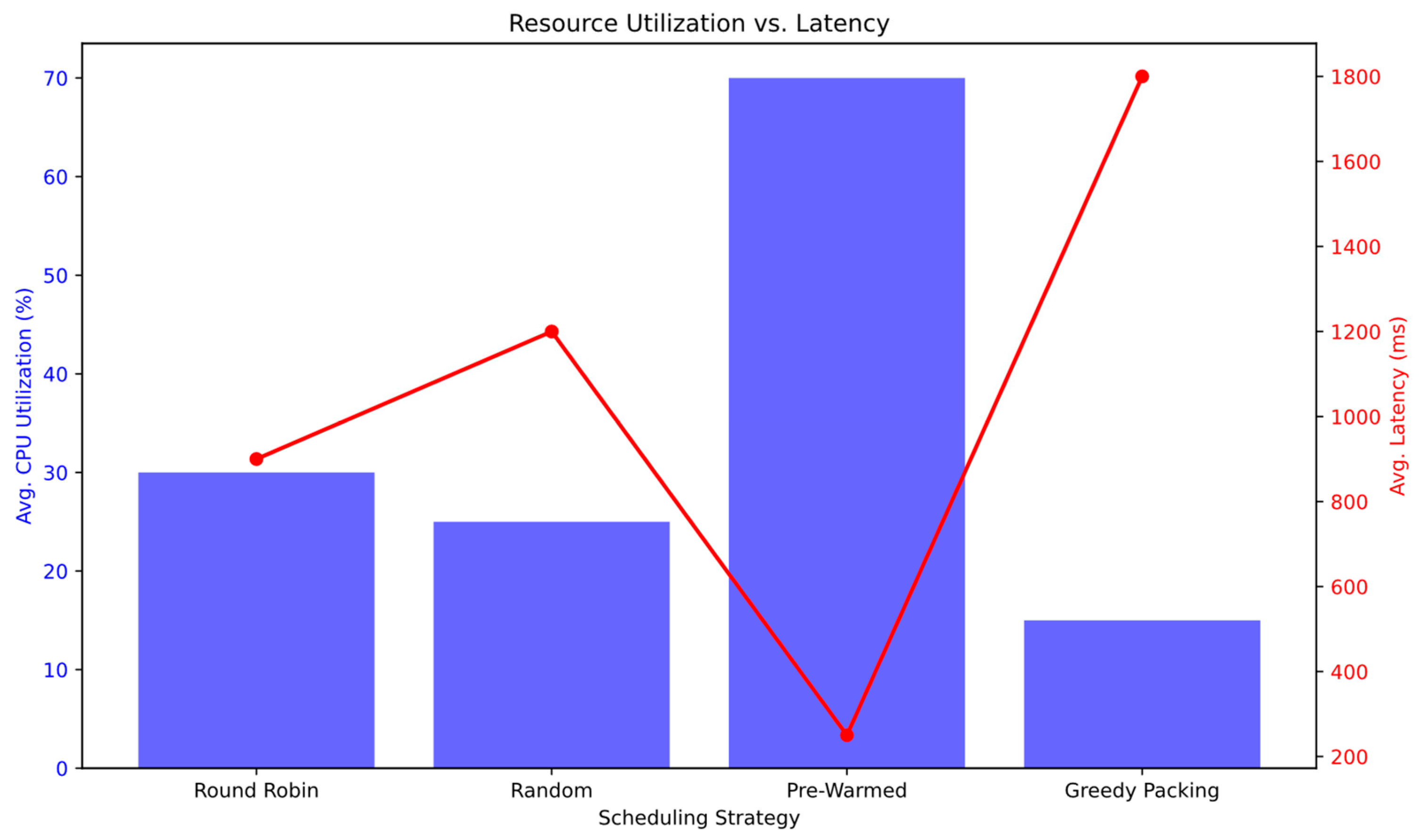
We conduct case studies to demonstrate how scheduling strategies directly impact resource utilization and latency in the serverless environment. Consider a scenario with four identical invokers, each with a capacity of 10 containers. The workload includes two phases: a steady phase with 20 invocations per minute for 5 min, and a burst phase with 200 invocations per minute for 5 min. Finally, four different scheduling strategies are used in this example as follows: Round Robin (RR), Random Selection (RS), Pre-Warmed (PW), which keeps five containers per invoker pre-initialized, and Greedy Packing (GP), which routes all invocations to a single invoker until it reaches full capacity. The results are presented in
Table 2.
The first observation is that all strategies except Pre-Warmed (PW) underutilize resources. For example, RR attempts to avoid overloading any single invoker by evenly distributing the workload across all invokers, but it fails to consolidate tasks for efficient resource use. RS shows similar results; its random assignment often creates “hotspots” where one invoker becomes overloaded while others remain idle, especially during the steady phase. This imbalance increases queuing time for the overloaded invoker and raises the frequency of cold starts, resulting in the worst latency (1200 ms). GP causes severe underutilization, with three invokers remaining idle throughout both phases and only 15% total CPU usage. On the other hand, PW—which resembles static provisioning—eliminates cold starts and achieves the best latency by using pre-warmed containers that absorb bursts of traffic. Its utilization results are significantly better than those of the other strategies. However, this comes at the cost of resource waste, as 20 pre-warmed containers remain unused during the steady phase. Another important observation is the relationship between latency and resource allocation, as shown in
Figure 2, which appears to be heavily influenced by cold start overhead, and latency decreases as resource readiness improves. When a sufficient number of pre-warmed containers is available (as in the PW case), cold starts are reduced or even eliminated, resulting in a significant drop in overall latency. However, this approach may lead to resource wastage and increased costs. Secondly, Resource Saturation: Overloading a single invoker causes increased queuing delays and sequential cold starts, both of which contribute to higher latency. From this simplified scenario, we can conclude that to minimize latency while maximizing utilization, schedulers must dynamically provision resources based on real-time demand.
An efficient scheduling policy must simultaneously address the distinct requirements of global resource balancing (across invokers) and local container optimization (within a single invoker). Centralized multi-objective algorithms have been adapted to tackle these challenges [
5]; however, this approach creates performance bottlenecks as the system scales because a single scheduler handles all objectives, such as load balancing, container reuse, and scaling [
13]. Another challenge faced by such single-tier centralized schedulers is conflicting scheduling objectives. For example, minimizing cold starts may require over-provisioning containers, forcing the algorithm to prioritize one objective over another and resulting in suboptimal scheduling decisions. These challenges motivate us to implement a two-tier scheduling solution that separates concerns into infrastructure-level (global) and task-level (local) optimization. Each layer uses tailored strategies to address the multidimensional requirements of serverless environments.
Finally, the scheduler must consistently maintain adequate resources to accommodate sudden spikes in invocations, especially since serverless platforms emphasize seamless scalability for handling fluctuating workloads.
3. Related Work
To reduce function cold starts, some research [
3,
6,
14] focuses on addressing the underlying factors contributing to cold start latency, such as CPU, memory, and network. These studies identify these elements and propose solutions aimed at optimizing their performance. In a related study [
15], the researchers argue that the network component is the dominant factor in cold start latency. They claim that the creation and initialization of network connections is a shared stage among most serverless functions and significantly contributes to cold start delays. Their proposed solution involves creating a pool of empty network containers (paused containers) that remain connected to the currently active containers and share the same network configuration, making them ready for immediate use when needed.
Some other works have focused on warming or prewarming the runtime in cache, based on the principle that caching containers can reduce initialization time. [
16] Present Faa
$T, a transparent auto-scaling distributed cache for serverless applications. Faa
$T maintains an in-memory cache for each active function, reducing initialization time by pre-warming the cache with objects likely to be accessed. Suo et al. [
17] proposed HotC, which aims to reduce cold start latency and optimize network performance by integrating an exponential smoothing model with a Markov chain approach to predict future demand and dynamically create a pool of active containers at runtime. While these scheduling strategies effectively reduce cold start rates, they do not consider the resource state, either within a single invoker or across multiple invokers, in their scheduling decisions. As a result, pre-warmed containers naturally compete with busy (active) containers for CPU and memory resources, which can overload certain invokers and increase load imbalance across the system. Although reducing cold starts is a primary goal of our research, the two-tier scheduling approach we propose aims to reduce resource contention by prioritizing invokers with the most balanced resource usage, thereby avoiding overloading invokers that could delay container initialization.
Several recent studies have applied load forecasting to proactively pre-warm a certain number of containers, thereby minimizing the occurrence of cold starts. For example, [
18,
19] implemented approaches using ARIMA as the prediction algorithm to forecast upcoming invocations and initialize containers in advance to handle the anticipated workload. They demonstrated that this approach can reduce latency; however, these studies used limited datasets that do not reflect real-world workloads, and they lacked experimental comparisons with other prediction models against ARIMA. While ARIMA is a powerful, lightweight time-series forecasting tool, it relies on a linear assumption, capturing only linear relationships in the data. In contrast, serverless workloads frequently exhibit non-linear patterns, such as sudden spikes during specific events or significant decay following bursts. These irregularities are often misforecasted by ARIMA and treated as random noise. Furthermore, ARIMA cannot explicitly incorporate contextual feature variables into the prediction model. These limitations motivated us to combine ARIMA with Random Forest (RF) to leverage ARIMA’s lightweight nature and ability to model temporal causality, while using RF to correct ARIMA’s linear bias by incorporating time-based features and lagged residuals.
Another prediction approach was introduced by [
20], which uses a lightweight regression-based incremental learning mechanism to anticipate workload fluctuations online. This method eliminates the need for individual profiling of each serverless function. Long Short-Term Memory (LSTM) is another well-documented forecasting method widely used in traditional cloud platforms [
4,
21]. In [
5], LSTM is employed as a time series prediction model to forecast function invocation times. This prediction serves as the backbone for initiating an adaptive warm-up pool of containers. To further optimize prediction accuracy, a fine-grained regression method is coupled with the LSTM. However, adapting LSTM for serverless environments poses challenges. LSTM requires dense and large datasets to perform efficiently. When workloads are sparse and bursty—as is common in serverless environments [
22]—this can lead to poor generalization or overfitting [
23]. Another important consideration is the computational overhead: LSTM demands intensive resources, including memory and processing capacity. These substantial computational requirements present a problem in real-time serverless settings where rapid scaling is critical. Lastly, due to their complex architecture, LSTM models are difficult to interpret, making it challenging to diagnose the causes of prediction failures.
The scheduling problem in serverless platforms has recently gained increased attention. Most research focuses primarily on resource optimization and latency reduction. Stein [
24] introduces a noncooperative online allocation heuristic (NOAH) scheduler designed to balance resources and response time effectively. Aumala et al. [
25] proposed PASch, a package-aware scheduling approach that assigns tasks based on package size to the least loaded, affinity-aligned node. During scaling operations, consistent hashing is applied to ensure fair redistribution of tasks. This design aims to reduce task launch latency and accelerate execution time. In Ensure [
26], functions are categorized dynamically online and then at the invoker level. A greedy scheduling algorithm is adapted to regulate CPU usage. Across invokers, Ensure aggressively directs load to an optimal number of invokers to enable container reuse, thereby minimizing the overall number of active invokers. The scaling strategy is based on queuing theory, allowing Ensure to proactively determine the required number of containers and invokers. However, this strategy—and similar proactive scaling methods that are “prediction-blind”—introduces a significant agility limitation when responding to dynamic workloads. Sudden changes can cause scaling delays, leading to increased cold start occurrences during spikes or wasted resources during sudden drops. In our work, we rely on predictive scaling to manage traffic spikes by using ARIMA+RF forecasts to scale invokers preemptively. Additionally, resource-aware scheduling helps eliminate hotspots. Finally, [
27] proposed a Multi-Queue Scheduling (MQS) algorithm for IaaS cloud environments, which classifies user requests into several distinct queues based on their burst durations.
4. Design Overview
4.1. Problem Formulation and Analysis
Consider function requests: , where each request of different types belongs to a function type and arrive at time . Each function type has unique characteristics, including execution time, cold start penalty, and resource requirements. Each request can be assigned to a warm container or a cold container to be processed. We define the variable if the request of type assigned to warm container and variable if the request of type assigned to a warm container. The problem of scheduling those requests under SLA latency constraints can be formulated as a Multiple Knapsack Problem (MKP) with additional constraints. The total knapsacks in our problem is the provider container limit and the constraints can be summarized as:
all requests must be assigned.
pre-warmed containers cannot exceed predictions.
the total containers that have been spawned is less than the provider resources limit in terms of CPU capacity and available memory (represented by total containers allowed).
Those constraints are formulated as follows, respectively:
We define the SLA violation indicator as follows:
where
is the latency for cold containers of function type
and
is the latency threshold for type
. Based on the assumptions above, the scheduling problem in serverless computing is formulated as maximizing the number of SLA-compliant requests:
4.2. Solution Architecture
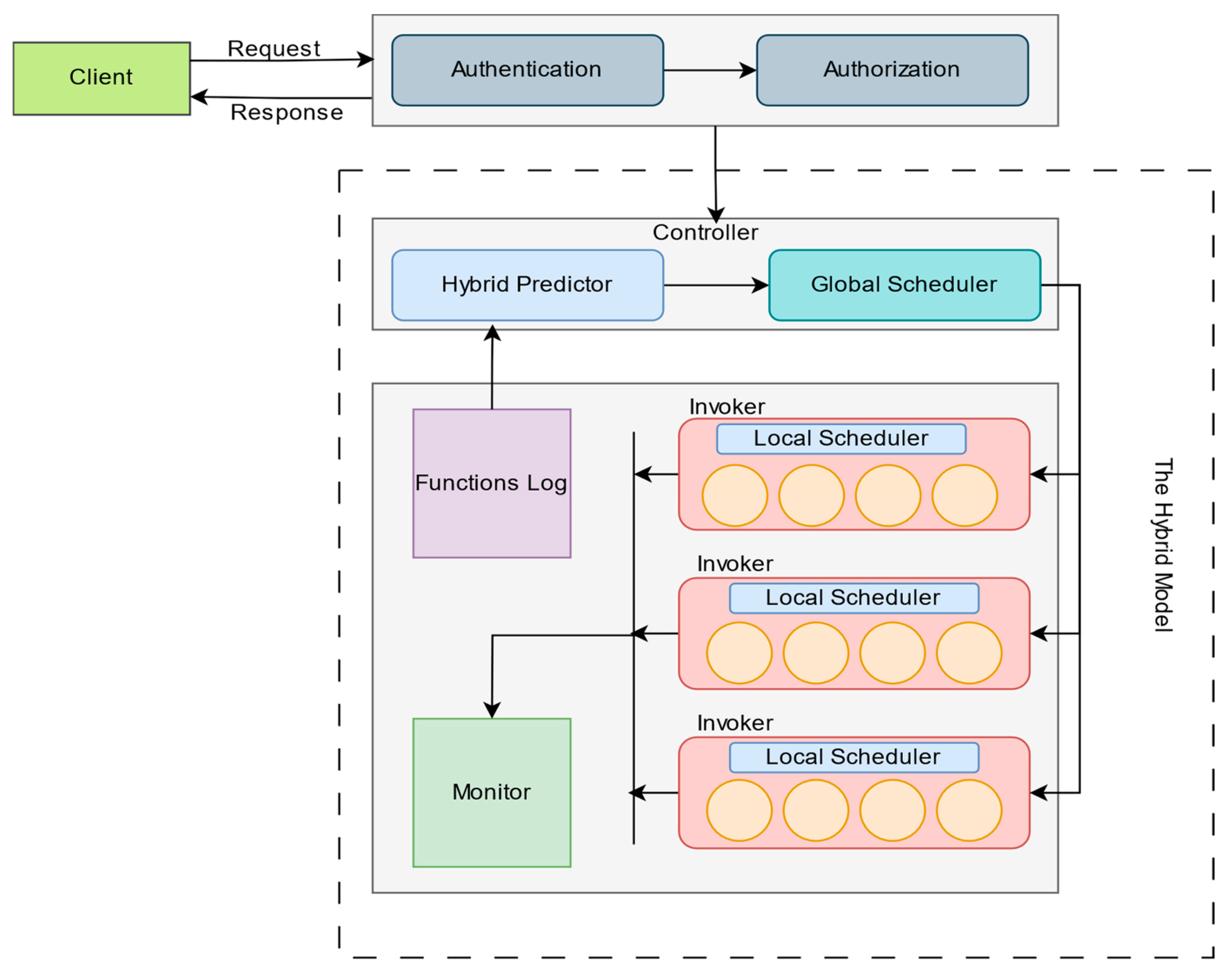
The model design is illustrated in
Figure 3. The core component of our system is the Controller, which comprises two main modules: the hybrid predictor and the global scheduler. The hybrid predictor forecasts future request arrivals based on historical data stored in the function’s log. It combines ARIMA and Random Forest (RF) prediction methods to produce a final, accurate forecast of request arrivals at specific times. The other key component is the global scheduler, responsible for routing requests to the most appropriate invoker among those available in the system. Additionally, the global scheduler manages scaling in and out of invokers based on the current resource status of each invoker. This resource states that information is maintained in the Invokers Info Table. At each invoker level, a local scheduler is deployed. This scheduler uses the hybrid predictor’s forecast as input and is fully responsible for managing the container pool within that invoker. The local scheduler combines the hybrid prediction with the current state of each container to decide whether there is a warm container ready to handle a request, if the request should be queued until a container becomes available, or if a new container must be spawned (resulting in a cold start). This decision-making process is based on a buffer-aware greedy approach, which is explained in more detail in
Section 6. Information about each request is stored in the function’s log, including execution time, resource usage (CPU and memory), and batch size. This data serves as a training set for the profiling model to estimate the expected execution time of specific functions. While the Hybrid Predictor serves as the brain of our system, its value emerges only when coupled with the Global Skewness-Aware Scheduler and Local Buffer-Aware Scheduler; without this integration, predictions alone cannot mitigate cold starts or balance infrastructure load. The Monitor component continuously tracks cold starts, latency, and resource utilization. It is also responsible for retraining the hybrid prediction model whenever performance degrades, specifically, when the RMSE increases by 10% in our experiments.
5. The Hybrid Predictor
A core objective of our solution is to minimize cold start occurrences. The first step toward achieving this is accurately predicting future load over a given time interval. Reliable forecasts allow the scheduler to pre-warm the required number of containers in advance, following the strategy that will be detailed later. Traditional time-series prediction models, such as LSTM, face significant limitations in FaaS environments. While LSTM can capture complex dependencies in invocation patterns, it requires a large volume of data for effective training and is computationally intensive. ARIMA, which has been widely used in various studies [
18,
19], struggles to incorporate exogenous variables (e.g., time of day, day of week) and cannot capture non-linear trends. Lastly, Prophet—which combines time series decomposition with machine learning fitting—often performs poorly in environments characterized by irregular or highly dynamic patterns. To address the limitations of standalone models in FaaS workload forecasting, we build a hybrid prediction model that combines ARIMA and Random Forest (RF). While hybrid ARIMA-RF models exist for time-series forecasting, this work pioneers their adaptation to serverless environments through environment-aware feature engineering and tight scheduler integration. This model serves as the forecasting component of our system. By leveraging the strengths of both ARIMA and RF, the hybrid model reduces forecasting errors and provides more robust predictions: ARIMA captures the linear base patterns, while RF corrects the residuals. This design is also highly adaptive, making it suitable for both steady-state workloads and bursty or spiky traffic.
Our hybrid predictor is specifically designed for serverless environments. The model consists of an ARIMA component that captures the linear patterns and a Random Forest component that models the non-linear residuals . The final prediction is produced by combining the outputs from both components.
5.1. ARIMA Model
The goal of this model is to minimize prediction error for linear time series data by capturing temporal causality. Temporal causality refers to a cause-and-effect relationship in which past data influence future outcomes in a time-ordered sequence. In ARIMA forecasting, this means that the value of a variable at time depends on its own past values () rather than on external factors. ARIMA () is specifically designed to model this relationship by analyzing historical data. The parameters are defined as follows:
p: the number of lagged observations included in the model, also called the AR/Auto-Regressive term.
d: the number of order differences that the time series data needs to achieve stationarity, also called the I/Integrated term.
q: the number of lags of the forecast error used in the forecast model, also called the MA/Moving Average term.
ARIMA
is formulated then according to Bowerman and O’Connell’s notion [
28] as follows:
where
is the Lag operator,
is (AR),
is (MA),
is the white noise error term and
is the differencing order used to achieve stationarity (I). The ARIMA model uses these three components—AR, MA, and I—to capture and identify linear temporal patterns in the data. Specifically, the AR component defines the relationship between the current value and its past (lagged) values, the I component ensures stationarity by removing seasonality and trend, and the MA component corrects the prediction based on past forecast errors.
During the training process, we use the Akaike Information Criterion (AIC) [
28] to select the optimal parameters
. The AIC is defined as:
where
is the likelihood of the model, and
. To achieve a better model fit and improve accuracy, we minimize the AIC value. The final step is to compute the residuals
as:
where
is the actual number of function requests at time
t. These residuals are the input that the RF works on and aims to correct.
5.2. Random Forest Model
The second component of our hybrid predictor is the Random Forest (RF) model. This model is used to correct the forecasting errors produced by ARIMA by detecting non-linear patterns in the incoming data. These non-linear patterns often arise from factors that influence workload but do not follow a clear temporal sequence—factors that ARIMA is unable to capture. Such factors may include external events, user behavior, or other contextual variables. To address these limitations, the RF model operates on an engineered feature set defined as , which includes:
Time-based features: These features capture periodic patterns or contextual influences that ARIMA cannot model directly, thereby accounting for time-sensitive external events.
Lagged residuals: represent historical prediction errors that ARIMA fails to capture, such as sudden workload spikes. Incorporating these residuals allows the RF model to compensate for ARIMA’s linearity assumptions.
We compute the non-linear residual
using Random Forest regression [
29], which averages predictions across
B decision trees:
where
is the
b-th decision tree. The final prediction of the hybrid model is the combination of ARIMA’s linear forecast and the RF’s correction of non-linear residuals:
where
represents undefined errors. The main advantage of this hybrid approach—coupling ARIMA with RF—lies in the RF’s ability to reduce the variance that ARIMA fails to model. This benefit is expressed as:
while ARIMA-RF hybrids exist in forecasting the literature, we design our predictor to suit the serverless environment specifically through incorporating RF with explicit time-based features that represent external events based on the domain knowledge, in addition to SLA-triggered retraining when cold starts exceed 5% or prediction RMSE is greater than 10%. These adaptations are essential for serverless, where infrastructure dynamics dominate performance.
5.3. Prediction Validation
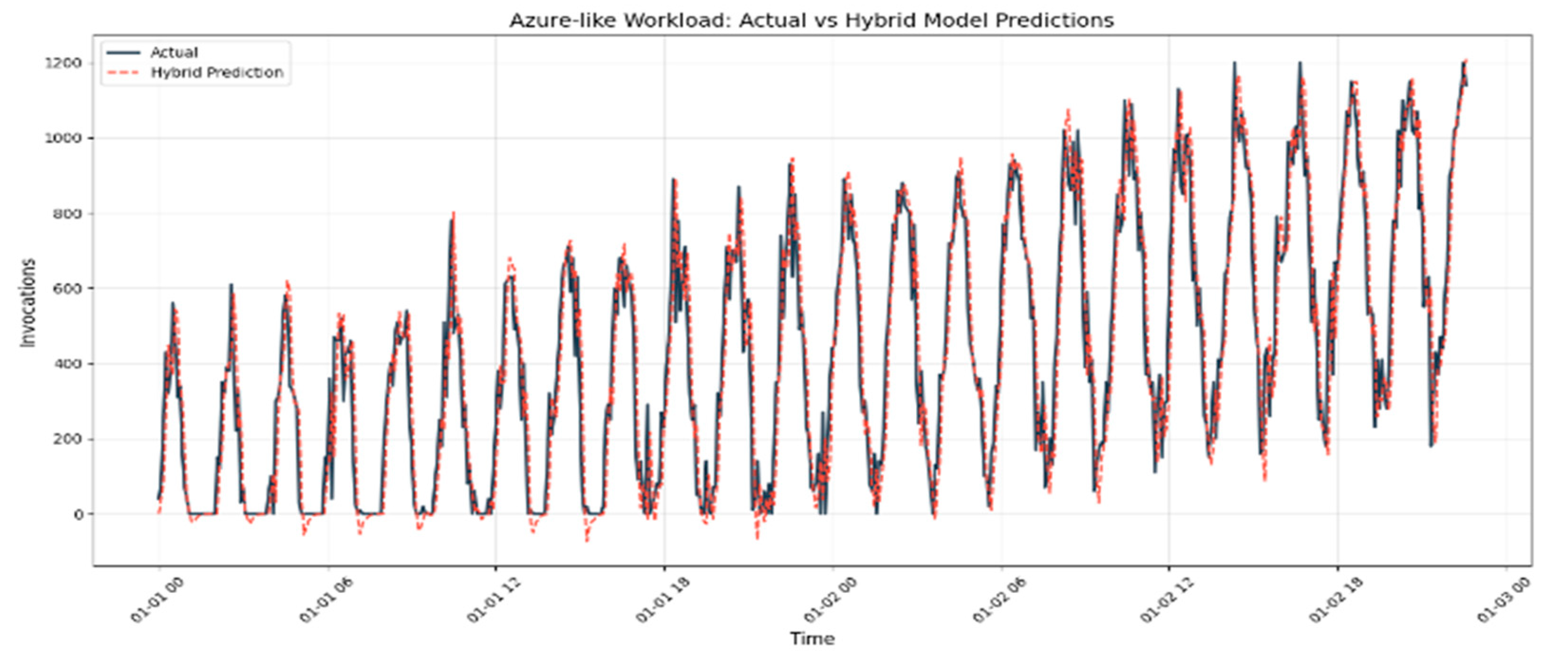
Dataset: To validate the hybrid model, we use a synthetic dataset (presented in
Figure 4) that mimics the Azure 2019 [
30] traces over 7 days, with a peak invocation rate of 1200 per second and an average of 300 per second, including some Gaussian noise. The invocations are generated with timestamps at 5-min intervals over 7 days, resulting in 2016 data points. The base workload is modeled using a Fourier series to capture cyclical patterns with additive seasonality and an upward trend. Spikes are modeled with Pareto-distributed magnitudes to simulate 10–100× surges: 90% of the spikes are 2–5× the base workload, and 10% are 10–15× the baseline (resembling extreme surges), with a 5% probability per hour (aligned with Azure’s burst frequency) of occurrence. The shape of the spikes is modeled as asymmetric Gaussian pulses to simulate rapid rise and decay. To simulate background noise, zero-mean Gaussian noise (σ = 15 invocations/second) is added to represent small fluctuations, along with impulse noise applied to 1% of the data points, multiplied by 10× to simulate outliers.
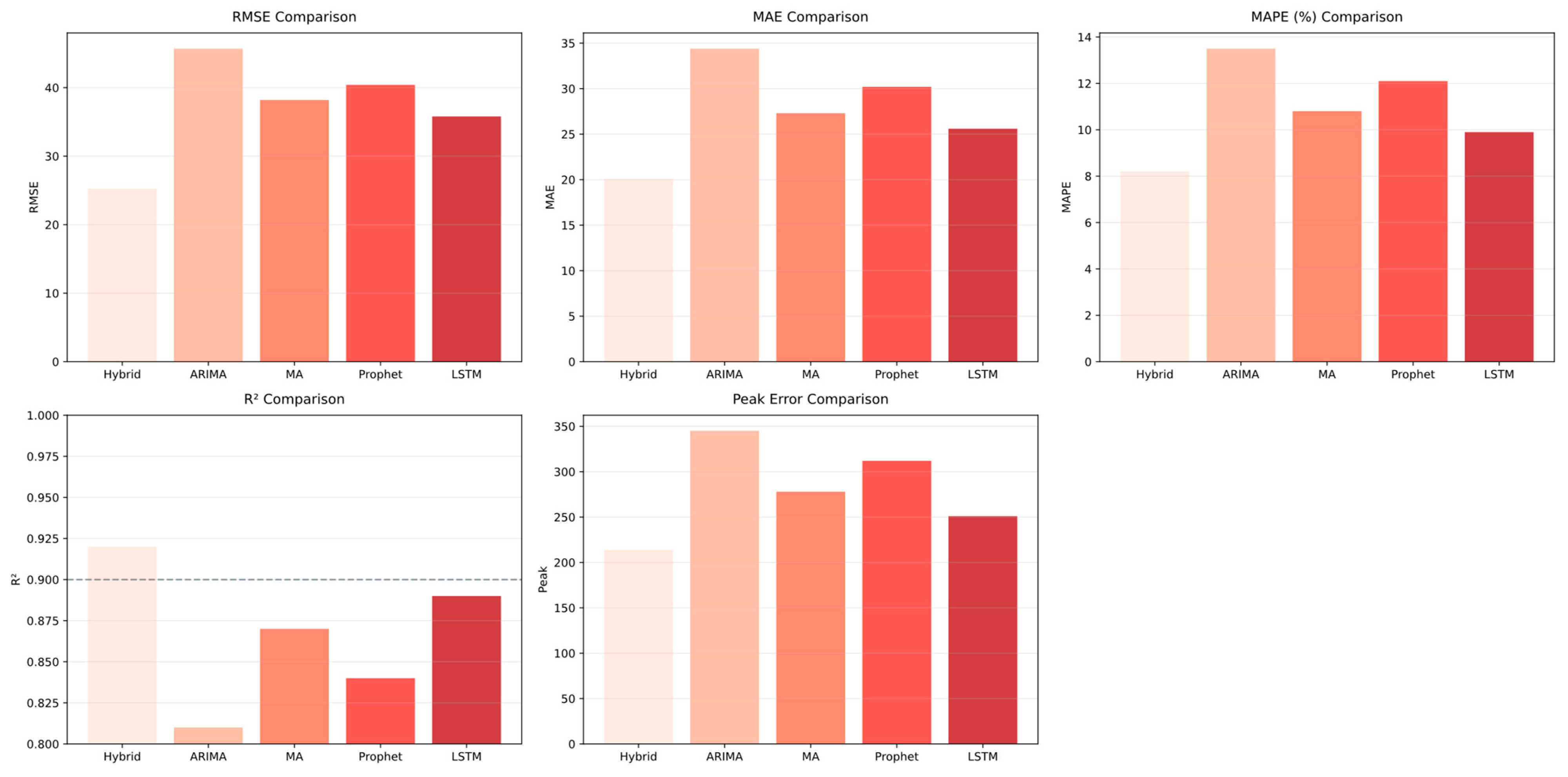
Metrics and Baselines: We used five metrics to evaluate prediction accuracy: Mean Absolute Error (MAE), Root Mean Squared Error (RMSE), Mean Squared Error (MSE), R-squared (R2), and Peak Error. Our hybrid prediction model was evaluated against several baseline strategies, including ARIMA, LSTM, Prophet, and Moving Average.
Results: The results presented in detail in
Figure 5, show that our hybrid model outperformed traditional prediction methods. It achieved a high level of accuracy, with up to a 35% reduction in RMSE compared to standalone ARIMA, and a 22% reduction compared to LSTM. While LSTM is effective at capturing long-term dependencies and complex sequential patterns, it requires a large amount of data to train properly. With limited or noisy data, LSTM is prone to overfitting, which can lead to higher RMSE values. In contrast, the RF component of our hybrid predictor leverages exogenous features to model sudden spikes, reducing dependence on dense temporal data. This leads to lower RMSE values, particularly during irregular events, reflecting better overall accuracy. On the other hand, Prophet uses an additive model (trend + seasonality + holidays) and assumes linearity. It struggles to handle workload surges that do not align with predefined seasonal or holiday patterns. As a result, Prophet tends to smooth out spikes, leading to significant errors during sudden bursts. The Random Forest component’s ability to explicitly model such bursts and capture lagged residuals from previous spikes is reflected in the improved Peak Error scores when compared to both LSTM and Prophet.
6. The Local Scheduler
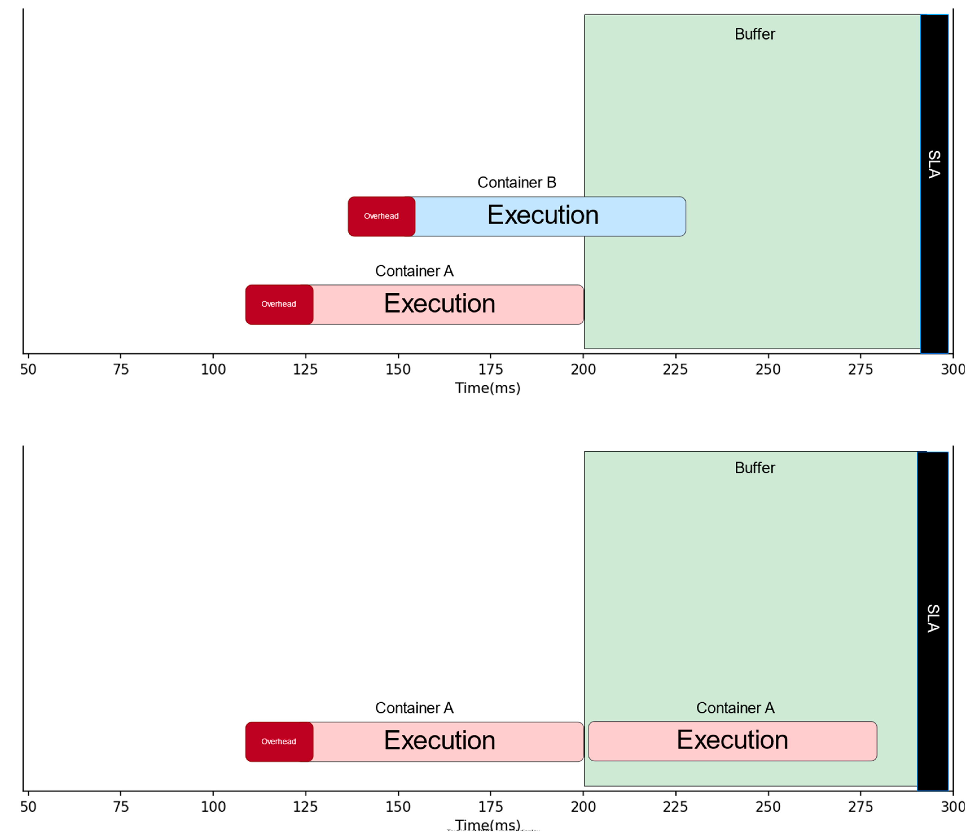
Within a single invoker, our scheduling strategy aims to maximize resource utilization while ensuring that SLA latency requirements are met. The key to achieving this is the aggressive reuse of available containers within the invoker, allowing a greater number of diverse incoming tasks to be processed concurrently without breaching SLA constraints. Pre-warming a set number of containers based on forecasted demand is an effective method for significantly reducing cold starts. However, this approach can increase the total number of active containers, potentially leading to underutilization of the invoker’s resources. In real-world serverless environments, application execution times vary widely, whereas SLA thresholds are fixed and based on latency constraints perceptible to users. Given that these applications often execute in just a few milliseconds, a substantial buffer (or slack) typically remains. The concept of slack, introduced by [
31], refers to the difference between a function’s actual runtime and its response latency. As shown in
Figure 6, if this available buffer can be accurately calculated, it can be leveraged to reuse an existing container instead of pre-warming a new one. To exploit this, we designed a buffer-aware greedy scheduling algorithm that utilizes both forecasting data and the currently available slack to determine which containers can be reused without violating response latency constraints.
In our approach, each container maintains a status: either busy or idle. When a request is assigned to a container, that container becomes busy for the duration of the function’s execution time. Knowing the execution time of a function task
on container
, we can calculate
(the expected ready time of container
). Based on this, the buffer-aware scheduler calculates the buffer vector
as:
Based on the forecast provided by the hybrid predictor, the scheduler must determine the estimated execution time for each predicted upcoming function The scheduler then assigns the function with the shortest expected execution time to the container with the longest available buffer vector—if and only if the total time threshold (the assigning condition). If no container has sufficient buffer to satisfy this condition, a new container is pre-warmed to serve the incoming function . This scheduling strategy (as shown in Algorithm 1) optimizes invoker resource usage by aggressively reusing current containers. Assigning the function with the shortest runtime to the container with the maximum buffer allows a single container to sequentially handle multiple functions. At the same time, enforcing the assigning condition helps minimize SLA violations. The assumption that SLA response constraints are typically greater than function runtime in serverless environments effectively transforms the scheduling challenge into an optimization problem.
Estimating the Execution Time
An important factor in the scheduling decision is accurately estimating the expected execution time of a given function. To achieve this, we perform controlled profiling on the four different applications used in our evaluation, as described in
Section 8.2. We assume that input size and required memory are variables provided by the user. For each function, we collect execution time data across various input sizes and memory configurations in a controlled environment (e.g., consistent CPU shares, warm starts only). This data is then used to train a regression model. Assuming input size and memory as predictors, each function is modeled using a simple linear regression of the form: Y: as a function of input size (
) and memory (
):
: Baseline execution time (intercept).
: Time per KB of input (slope for ).
: Time saved per MB of memory (Slope for ).
: Residual error.
By combining offline profiling with linear regression, we can reliably estimate the execution times of repetitive serverless tasks, allowing the buffer-aware scheduler to optimize resource utilization within the invoker.
| Algorithm 1: Local Scheduler |
| Input: |
| Output: L (final scheduling map within Invoker ). |
| 1: | foreach Request in do |
| 2: | Get all active containers |
| 3: | Calculate buffer vector |
| 4: | Calculate expected execution |
| 5: | if < |
| 6: | ← |
| 7: | end if |
| 8: | else |
| 9: | Cold-Start ← |
| 10: | end foreach |
| 11: | end |
7. The Global Scheduler
When the request demand exceeds the capacity of a single invoker, a new invoker must be added to the system to prevent overloading, which could lead to SLA violations. Conversely, when the load decreases, some invokers should be removed to avoid overprovisioning and wasting resources. Therefore, scheduling decisions across multiple invokers become a scaling-in/out problem. Although live migration has been proposed as a solution to this issue, it is not suitable for integration with our buffer-aware scheduler. This is because, even when the hybrid predictor provides accurate forecasts, our scheduling decisions rely not only on invocation predictions but also on the expected buffer length, making live migration incompatible with our approach.
To address the scaling problem in relation to the buffer-aware scheduler, we introduce a skewness-aware model designed to prevent both over- and under-provisioning of available resources. Skewness [
32,
33] is a widely used metric for quantifying uneven resource utilization. We extend this concept to the FaaS environment, where it represents the imbalance in workload distribution across invokers. In our model, we develop a new measure called the “skewness score,” which guides scaling-in and scaling-out decisions. Let’s assume that we have
types of resources (memory, CPU, storage), denoted as
. For each invoker, we calculate the skewness of resource
using the adjusted Fisher–Pearson coefficient of skewness as follows:
where:
is the resource
utilization (e.g., CPU%, memory GB, duration ms) at the
-th time point,
is the mean utilization over time series
and
is the sample standard deviation of the time series.
Then we create a composite score for each available invoker that weights resource skewness, variability, and utilization as the Skewness Score
for invoker
:
The skewness score serves as the primary indicator in the scaling process. A high score indicates greater skewness, suggesting that the invoker is more likely to experience resource starvation. Scaling decisions are made based on the skewness scores of all active invokers prior to routing the predicted incoming request. The skewness-aware algorithm (shown in Algorithm 2) computes the score for each available invoker, and the request is routed to the one with the lowest skewness score, representing the most balanced (i.e., stable) resource utilization. If all current invokers have reached full capacity and cannot handle additional requests, a new invoker is activated. In our experiments, we used three resource types to calculate the skewness score: CPU, memory, and execution duration.
| Algorithm 2: Global Scheduler |
| Input: |
| Output: G (final scheduling map across invokers). |
| 1: | foreach Request in do |
| 2: | Get all active invokers |
| 3: | Calculate skewness score |
| 5: | if < |
| 6: | ← |
| 7: | end if |
| 8: | else |
| 9: | Active new invoker |
| 10: | ← |
| 11: | end foreach |
| 12: | end |
The hybrid model scheduling approach establishes a clear separation of concerns between the global and local tiers, connected through a coordinated feedback loop. The Global Scheduler focuses on infrastructure-level decisions, routing requests to invokers based on their skewness scores, which reflect resource imbalances. It does not track individual requests, ensuring that its complexity remains scalable and unaffected by the number of active requests. The Local Scheduler, guided by the Hybrid Predictor forecast, is responsible for assigning tasks to containers with the largest available buffer and proactively pre-warming containers. It also updates the invoker’s resource state (CPU, memory, execution duration) and stores real-time resource metrics in the Invoker Info Table. Meanwhile, the Global Scheduler continuously monitors this table to recalculate skewness scores and adjust routing decisions accordingly. This layered architecture enables both efficient global infrastructure scaling and fine-grained local optimization, while maintaining overall scalability and adaptability.
8. Evaluation
8.1. Setup
We implemented our model on top of OpenWhisk, an open-source cloud platform. OpenWhisk consists of a REST interface for submitting functions and retrieving execution responses. The Controller is responsible for routing incoming function requests to the appropriate Invoker for execution. We modified the Controller by integrating both the Hybrid Predictor and the Skewness-Aware Scheduler. On each Invoker, we implemented the Buffer-Aware Scheduler, which manages the containers within the invoker. When a request arrives, we validate the API key and namespace permissions using OpenWhisk’s built-in authentication system and then update the Function Log with the new request data. We replaced OpenWhisk’s default Controller with a custom version that includes the Hybrid Predictor as a submodule. The Hybrid Predictor uses historical function logs (stored in CouchDB 3.3) to forecast the invocation count per function for the upcoming time window (5 min in our experiment). Additionally, we replaced OpenWhisk’s default Sharding Container-Pool Balancer with our custom Global Scheduler, which retrieves real-time metrics (CPU, memory, execution duration) from all invokers to compute the Skewness Score, and routes requests to the invoker with the lowest score. We added a new module, the Invoker Metrics Collector, which uses custom HTTP endpoints on each invoker to collect real-time resource metrics and store them in Redis 7.2.4 for low-latency access. To improve communication efficiency, we replaced OpenWhisk’s default pull-based model—where invokers fetch tasks from Kafka—with a push-based routing mechanism using gRPC v1.7 streams. This allows direct communication between the Controller, the Invoker Metrics Collector, and the Invokers. Additionally, on each invoker, we replaced the default ContainerPool with the Local Scheduler, which monitors the available buffer in each warm container. It assigns tasks to containers with sufficient buffer or triggers a cold start when necessary.
The modified OpenWhisk setup runs on a single server equipped with a 32-core Intel Xeon Platinum 2.80 GHz CPU and 250 GB of RAM. The operating system used is Ubuntu Server 16.04, and all functions are generated and executed on the same host.
8.2. Workload and Traces
We generated synthetic data that mimics the Azure 2019 Serverless Traces Dataset for simulation purposes. This dataset includes invocation patterns, temporal features, and noise, as described in
Section 5.3. To validate our model using real-world serverless functions, we used FunctionBench [
34] and Ensure [
26] to obtain the workload of four applications: Image Resizing (IR), Email Generation (EG), Prime Number computation (PN), and Matrix Multiplication (MM). These applications were selected based on their runtime and memory requirements. The first two, IR and EG, are short-lived applications, while PN and MM are long-running and resource-intensive.
8.3. Baselines
We compared our model against three baseline methods: OpenWhisk Default, Least Connection, and Hot Concurrency. A brief explanation of each method is as follows:
Hot Concurrency (HotC): Hot Concurrency refers to maintaining “warm” function instances to handle multiple concurrent requests [
17], representing a proactive warm-container scheduling mechanism.
Least Connection (LC): directs new requests to the instance with the fewest active connections. In the context of FaaS, this method distributes invocations to the least busy containers [
35], prioritizing load balancing in the scheduling decision. The
OpenWhisk default (OW): employs a pull-based model, where invokers retrieve tasks from a message queue as they become available, functioning as a reactive scheduling mechanism [
9].
9. Results and Discussion
9.1. Number of Containers and SLA
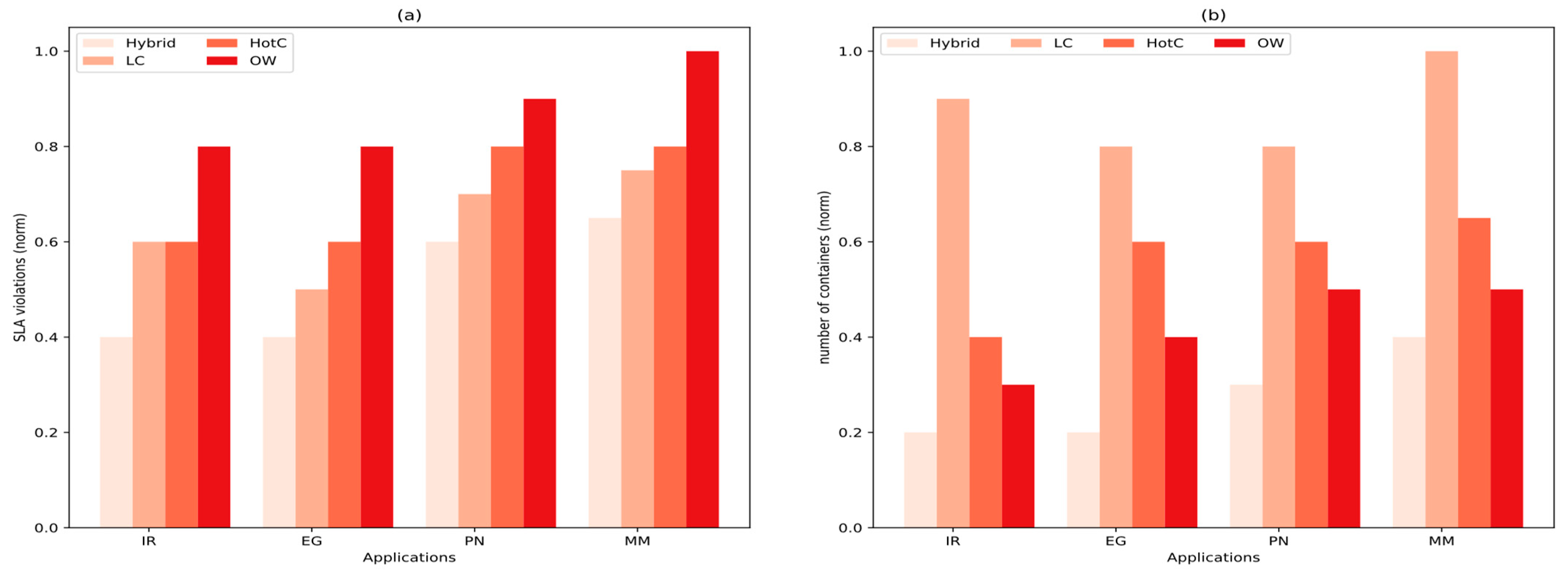
One of the key motivations behind designing the hybrid model was to minimize the number of containers while simultaneously reducing SLA violations. The results, shown in
Figure 7, demonstrate that the hybrid model successfully achieved this objective across all workloads. Its aggressive reuse of available containers resulted in spawning 20% fewer containers than OpenWhisk, even in the matrix multiplication (MM) case. OpenWhisk was the second-best performer in terms of reducing the average number of containers spawned, but this came at the cost of the highest SLA violation rate compared to all other baselines. While Hot Concurrency maintained an acceptable SLA, it did so by keeping a large pool of idle instances ready to handle bursts of traffic, which led to a high number of active containers. By combining accurate predictions with a proactive, container-aware scheduling mechanism, the hybrid model achieves a clear balance between container efficiency and SLA guarantees.
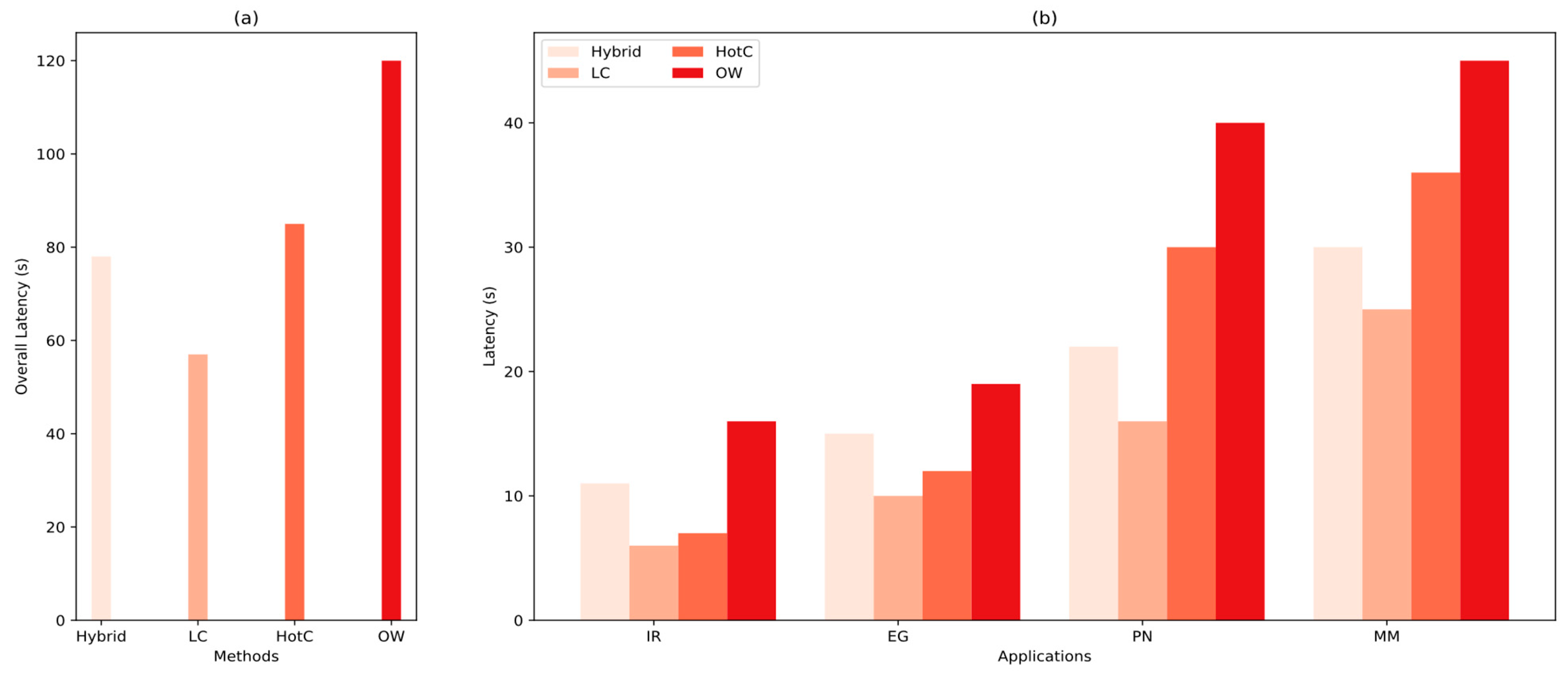
9.2. Overall Latency
We evaluated the overall latency of our system in comparison to the baseline methods, as shown in
Figure 8a. The Least Connection (LC) method demonstrated the lowest overall latency, with approximately an 18% improvement over the hybrid model. Hot Concurrency (HotC) showed comparable performance to the hybrid model, while OpenWhisk (OW) performed the worst due to its inability to handle sudden spikes in workload effectively. A more detailed examination of each workload’s latency, presented in
Figure 8b, reveals that although HotC achieves lower latency than the hybrid model in the IR and EG workloads, the hybrid model outperforms HotC in the MM and PN workloads. LC maintains the lowest latency across all workloads when compared to both the hybrid model and the other baseline methods. However, these results must be interpreted in the context of container utilization and SLA violation rates. In other words, while LC and HotC (particularly under lighter workloads) offer reduced overall latency, they do so at the expense of higher SLA violations and less efficient use of available containers.
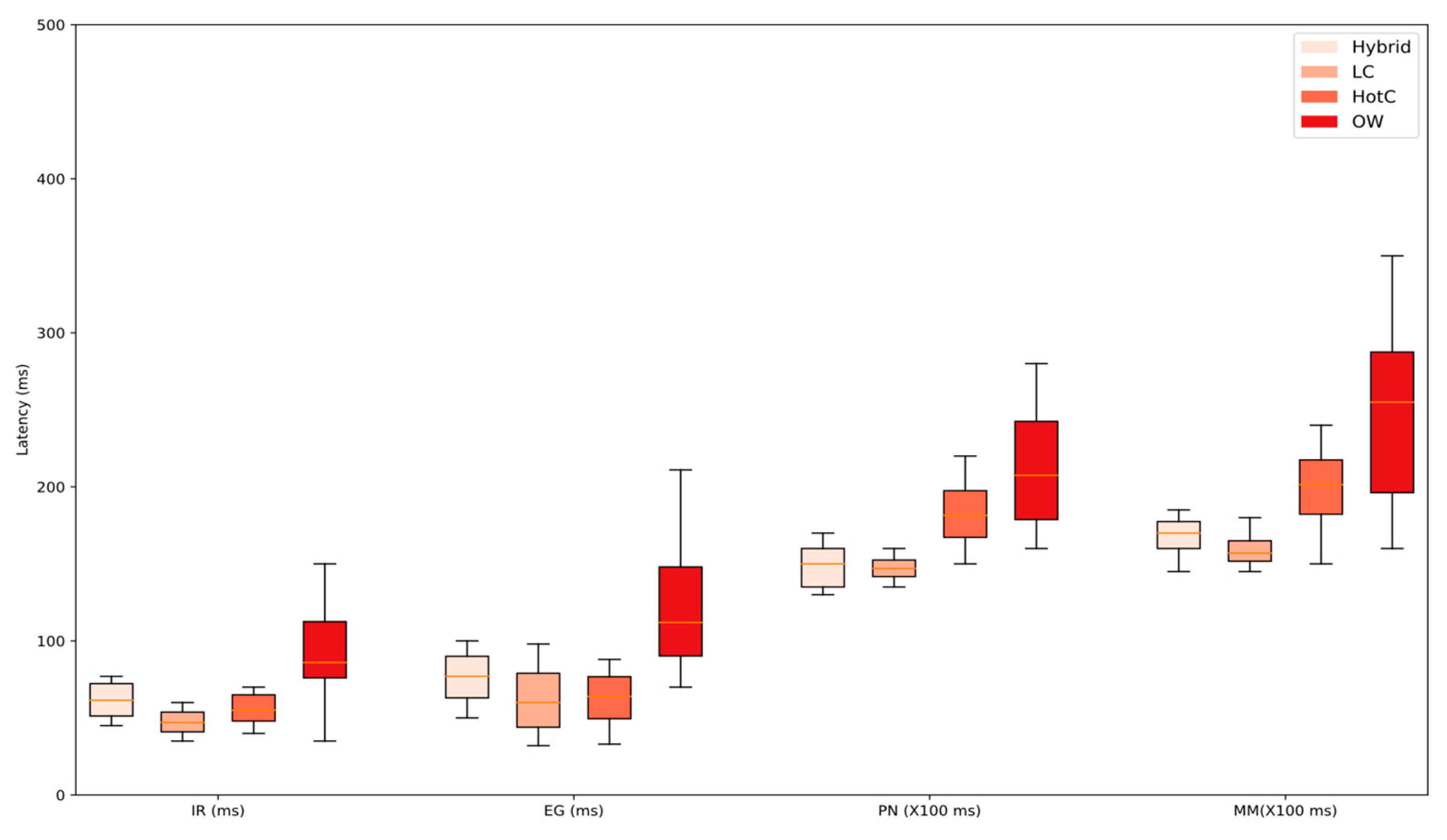
9.3. Tail Latency Analysis
Figure 9 presents the evaluation of tail latency (99th percentile) and latency-sensitive performance across each workload. The analysis reveals two behavioral patterns of our model. For short-lived applications, the hybrid model shows the second-highest latency, up to 2× that of LC (best) and 1.5× that of HotC. However, for resource-intensive workloads, the hybrid model improves significantly, becoming the second-best performer. In both cases, the higher median latency compared to other methods is expected due to the queuing overhead introduced by the buffer-aware scheduler. This overhead is more noticeable in short-lived applications because of their very short execution time.
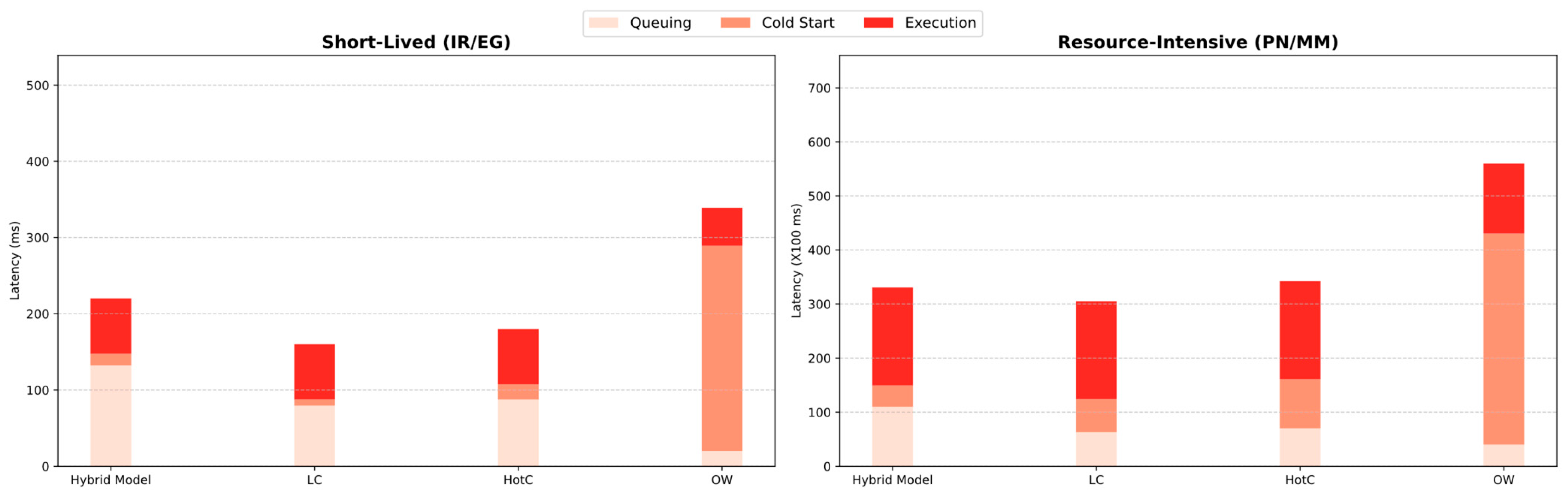
For a deeper analysis and understanding of these results, we break down tail latency (99th percentile) into three components: queuing time, cold start overhead, and execution time. We then compare tail latency (P99) for both short-lived and resource-intensive functions to assess the contribution of each component. The results (
Figure 10) show that OW suffers from frequent cold starts in both cases, resulting in the highest overall latency despite having the shortest queuing delay. In contrast, the hybrid model exhibits the longest queuing time among all baselines. This queuing overhead—up to 60% of total latency in short-lived functions—is due to the buffer-aware scheduler, which holds requests until warm containers become available. This strategy minimizes cold starts across all cases—7% in short-lived workloads and 14% in resource-intensive functions. However, in the short-lived case, it noticeably increases the waiting time for these brief tasks compared to HotC, which experiences more cold starts. While avoiding cold starts ensures more consistent latency for most users, requests that fall within the 99th percentile experience significant queuing delay (132 ms), which can be problematic for latency-sensitive short tasks. In contrast, under compute-intensive workloads, the hybrid model shows improved tail performance (second only to LC). Although it continues to incur the highest queuing time (nearly twice that of HotC), it significantly reduces cold start occurrences, which is critical for handling resource-intensive functions efficiently.
That said, despite the increased median latency, SLA violations remain within acceptable limits, as previously demonstrated. Moreover, the number of spawned containers is significantly lower than in methods with shorter median latency. For instance, the hybrid model spawns up to 60% fewer containers than LC, the method with the lowest median latency.
9.4. Improvement in Cold Start
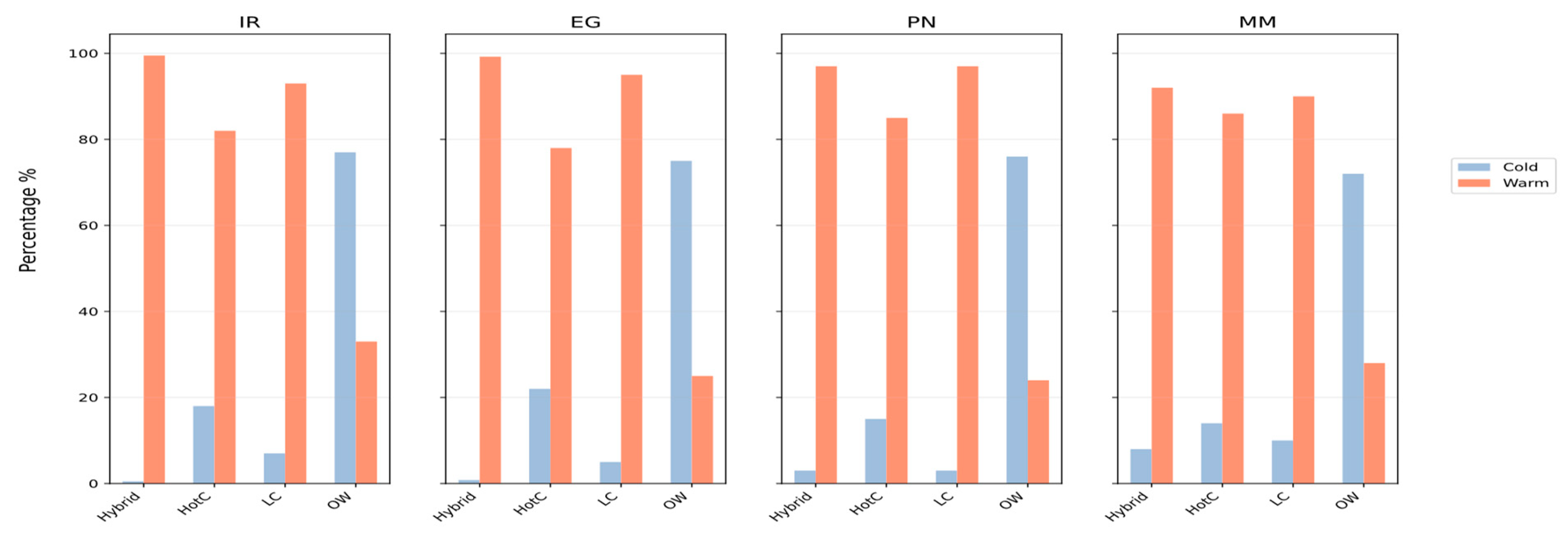
We analyzed our trace data to examine the execution characteristics of incoming requests. The results, shown in
Figure 11, indicate that the hybrid model achieves the highest percentage of warm starts and the lowest cold start overhead, reflecting an aggressive reuse of available containers. Specifically, 97% of all requests are assigned to warm containers. Although the cold start overhead increases for resource-intensive applications (reaching 8% in the MM case), the hybrid model still outperforms all baseline methods. In contrast, OpenWhisk exhibits the highest cold start overhead across all scenarios, with 75% of requests triggering cold starts. HotC delivers generally strong performance but maintains a lower warm start percentage in the MM and PN workloads. The cold-to-warm start ratio plays a crucial role in determining overall latency. In optimal scenarios, where all requests are handled by warm containers, latency consists only of execution time and queuing delay, both of which are minimal due to the lightweight nature of serverless functions. However, as the cold start ratio increases, a fixed initialization penalty is introduced. This overhead significantly inflates latency, and its cumulative effect becomes the dominant factor in average response time. Therefore, reducing the cold start ratio is essential for maintaining low latency, as confirmed by the results shown in
Figure 8 and
Figure 11.
Although the number of cold and warm starts does not necessarily reflect the overall system performance—as previously noted, LC achieves the lowest latency, and HotC performs slightly better in certain scenarios—a complete performance picture emerges when we also consider invocation execution and SLA violations. This analysis aligns with the core principle of the buffer-aware scheduler, which prioritizes reusing warm containers over minimizing latency, provided that SLA constraints are not violated.
9.5. Container Utilization
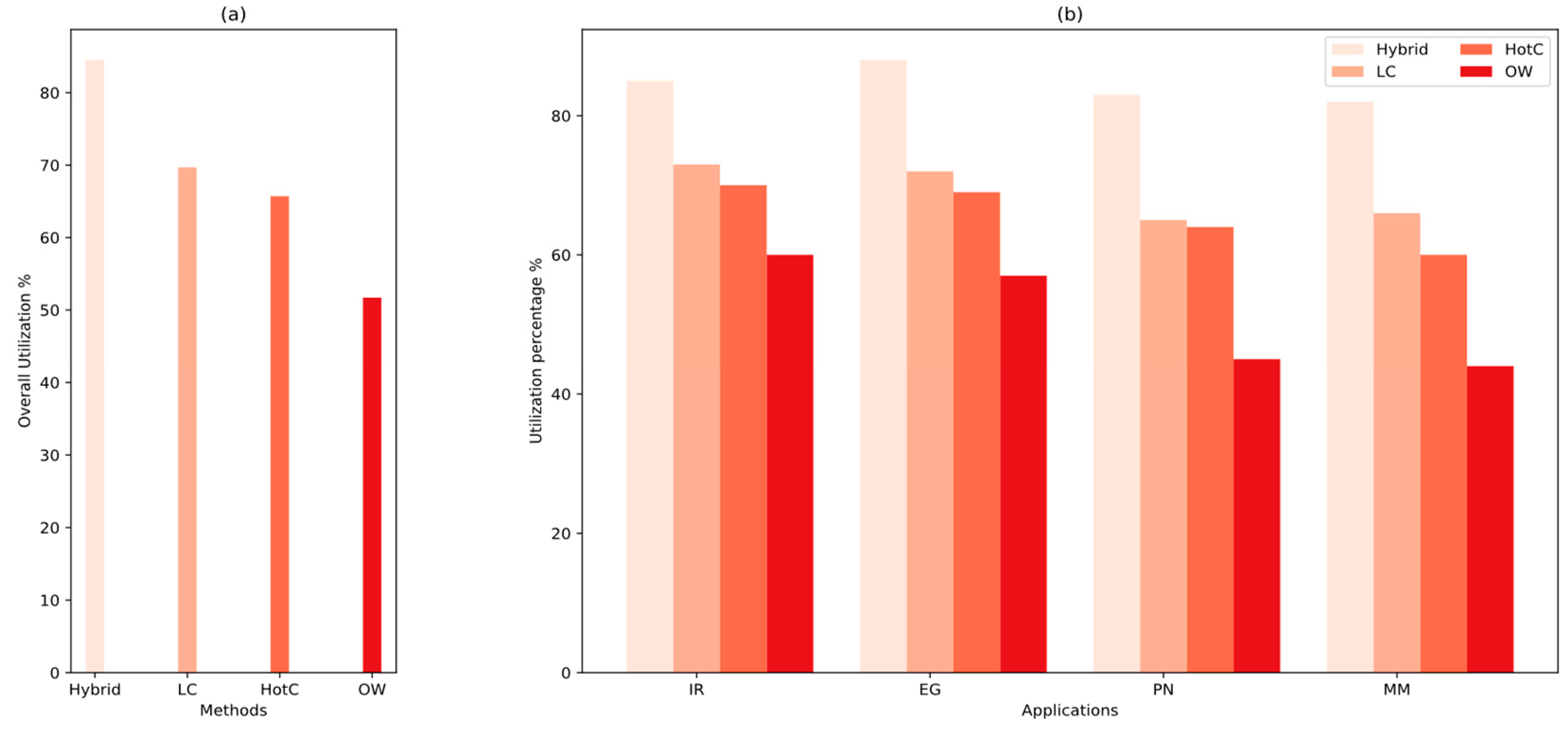
We calculate utilization as the percentage of time containers are actively processing requests, excluding periods of inactivity after the last request until the container times out. Higher utilization indicates more efficient resource use, as it means fewer resources are sitting idle.
Figure 12 presents a detailed evaluation of container utilization across the four test applications. The Hybrid model consistently achieves over 80% utilization regardless of workload type. This improvement is attributed to the Hybrid Prediction Model, which enables accurate proactive scaling and the aggressive reuse of containers by leveraging available buffer capacity. The most notable gains are observed in long-lived applications. This enhanced utilization also translates into a smaller container fleet size, as the Hybrid model requires fewer containers to handle the same workload, as previously discussed.
9.6. Cold Start Penalty Scaling Analysis
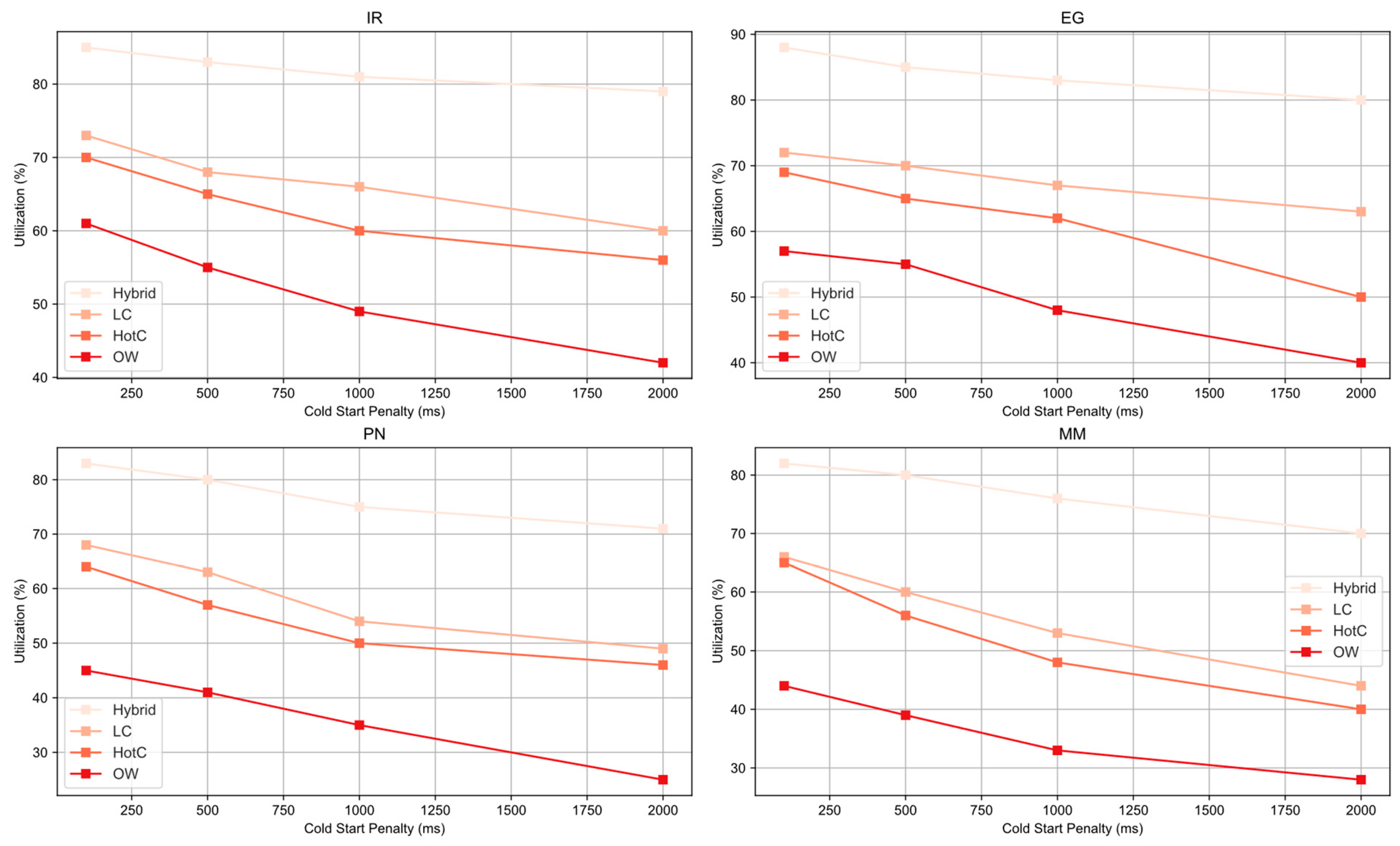
Cold Start Penalty Scaling Analysis evaluates how system performance deteriorates as the cost—measured in time or resource overhead—of initializing a new container (cold start) increases. This analysis involves systematically introducing artificial delays (ranging from 100 ms to 2000 ms) during cold starts and measuring the resulting impact on container utilization. The results, presented in
Figure 13, show that the Hybrid model’s performance degrades more gradually than the other methods across all application types. The most significant drop in utilization for the Hybrid model occurs in the PN and MM workloads, at approximately 12%. In contrast, some methods, such as OW, show up to a 20% degradation in similar scenarios. This more graceful decline in performance indicates that the Hybrid model’s proactive strategy—combining pre-warming and buffer-aware scheduling—is effective across varying workloads and cold start penalties.
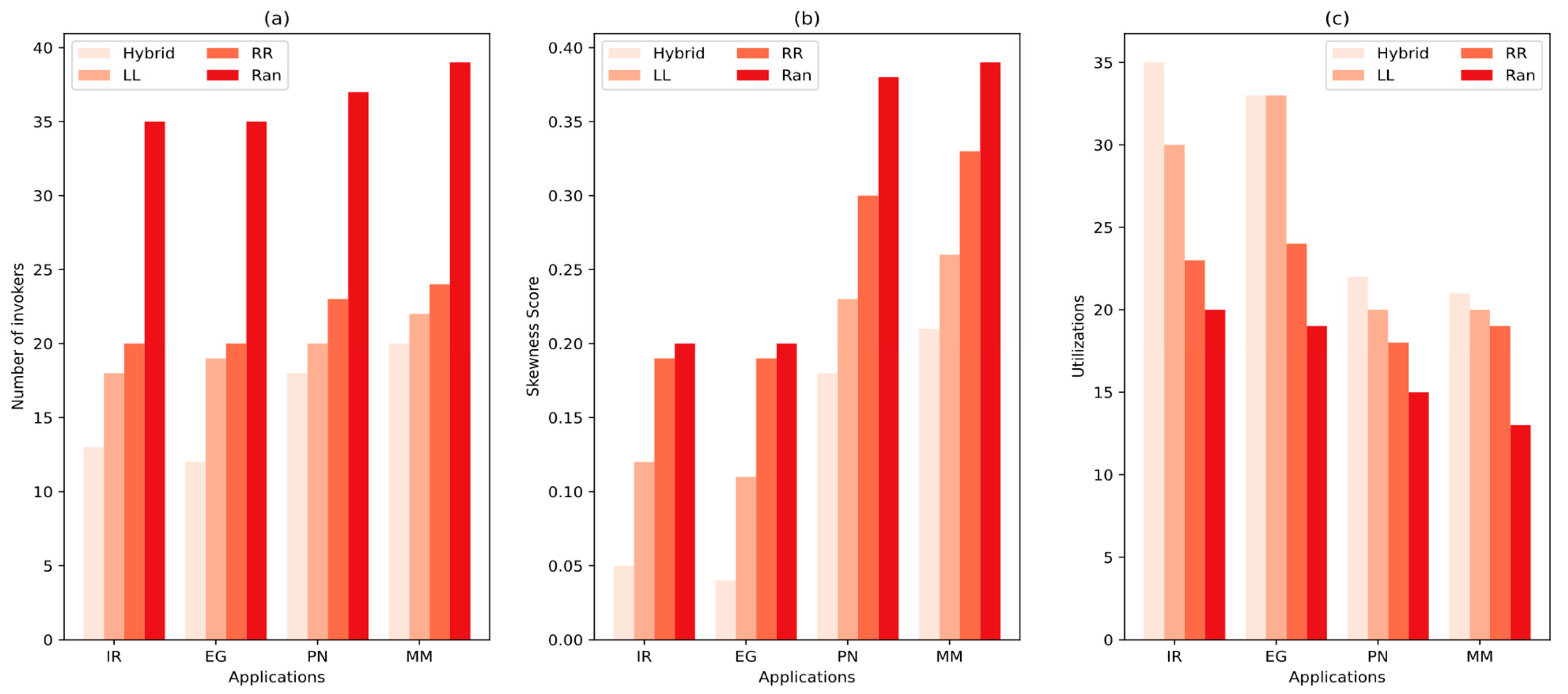
9.7. Multi-Invoker Scheduling
To validate the performance of the hybrid model using the synthetic dataset in complex multi-invoker environments, we assess its ability to optimize resource efficiency by minimizing the average number of invokers used while maximizing their resource utilization. For this evaluation, we compare the hybrid model to commonly used baseline load-balancing methods in both research and industry for distributing function requests across available invokers: Round Robin (RR): Distributes requests sequentially across invokers in a fixed rotation. This method is simple to implement and ensures an even distribution under steady workloads. Least Loaded (LL): Routes requests to the invoker with the shortest queue or fewest active requests. LL adapts to real-time load and reduces queuing delays. Random (Ran): Assigns requests to invokers randomly without tracking state. This method is stateless and lightweight.
The results of the four methods across the four workload types are presented in
Figure 14. Based on these results, several observations can be made from
Figure 14a: both RR and LL significantly reduce the number of active invokers compared to the Random (Ran) load-balancing strategy. Notably, LL initializes approximately 40% fewer invokers than Ran across all workload scenarios. The hybrid model achieves even further reductions in the number of active invokers, ranging from 27% in short-lived workloads to 8% in resource-intensive workloads. Additionally, we observe that in resource-intensive workloads, the hybrid model’s performance converges with that of LL; however, it consistently requires the fewest invokers for the same workload across all scenarios. These results demonstrate that the combination of hybrid prediction and skewness-aware scheduling effectively reduces the required resources—specifically, the number of invokers—by preventing resource starvation in serverless environments. In
Figure 14b, we use the median skewness score to validate the efficiency of resource provisioning. The lower average skewness score achieved by the Hybrid Model indicates more effective and balanced resource allocation. Finally, in
Figure 14c, the Random (Ran) algorithm shows clear underutilization of available resources, while both the Hybrid Model and the Least Loaded (LL) method demonstrate more balanced allocation. This balanced distribution contributes to a reduced number of active invokers.
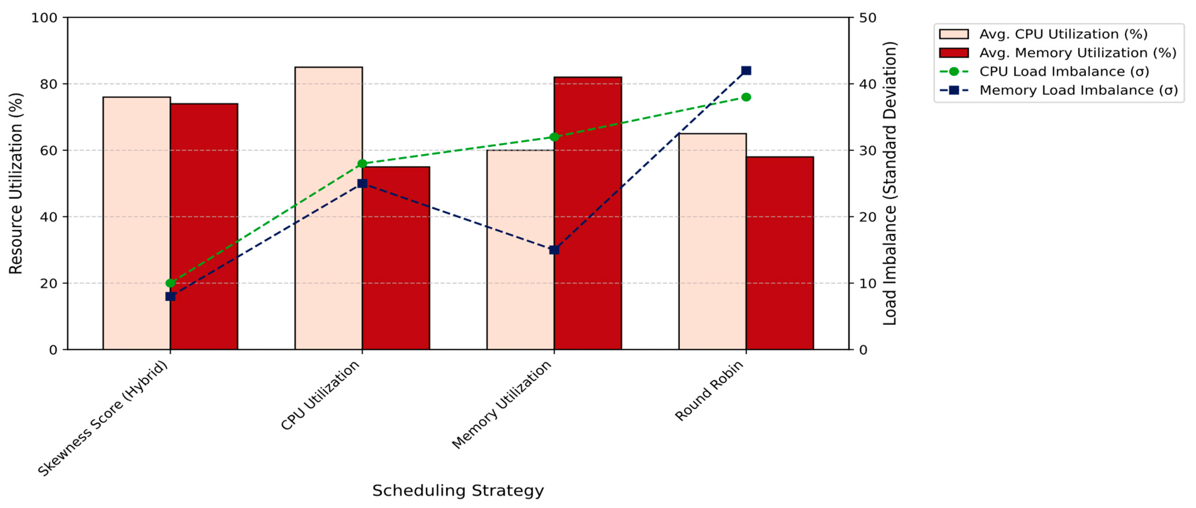
9.8. Skewness Score Performance Analysis
In this section, we compare the Hybrid Model’s skewness-aware scheduling approach (Skewness Score) against utilization-driven strategies—specifically, CPU Utilization, which routes requests to the invoker with the lowest CPU usage, and Memory Utilization, which selects the invoker with the lowest memory usage. We also include Round Robin as a baseline that represents a lack of resource awareness.
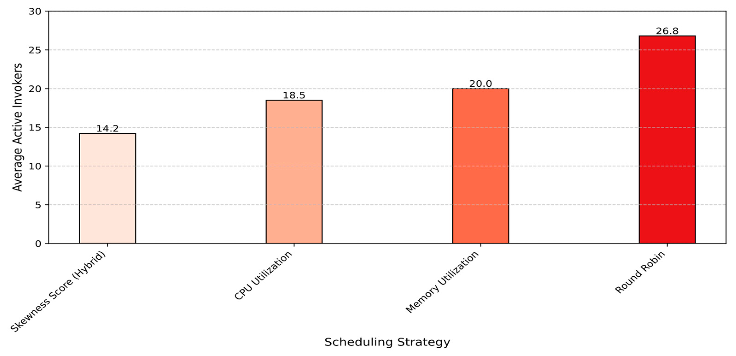
Figure 15 shows that relying on single-resource metrics (CPU or Memory) while ignoring the interdependence between resources leads to inefficiencies. For example, the Memory Utilization method underutilizes the CPU (62%), while the CPU Utilization method causes CPU overloading (88%). In contrast, the Skewness Score approach accounts for multiple dimensions—CPU, memory, and execution duration—resulting in more balanced usage, with CPU and memory utilizations of 78% and 75%, respectively. This helps avoid both resource underutilization and bottlenecks. Another factor used to evaluate these strategies is load imbalance, measured by the standard deviation of CPU and memory usage. The skewness-aware approach significantly reduces load imbalance for both CPU and memory compared to the severe imbalance caused by Round Robin’s static distribution. A low imbalance indicates that the workload is evenly distributed across invokers, preventing any single invoker from being overwhelmed or forming performance hotspots. This improvement in resource utilization directly impacts the number of active invokers required to handle incoming requests. As shown in
Figure 16, the Hybrid Model requires the fewest invokers—only 14—demonstrating the effectiveness of skewness-aware routing in maximizing resource efficiency. In contrast, Round Robin requires nearly double the number of invokers, while CPU and Memory Utilization strategies need 4 to 8 additional invokers due to the bottlenecks they introduce.
10. Conclusions
This paper presents the Hybrid Model, a novel serverless solution designed to enhance scheduling and resource management in serverless platforms. The Hybrid Model provides accurate forecasting of upcoming workloads and applies a two-stage scheduling strategy based on these predictions to reduce cold start occurrences and mitigate their negative impact on resource provisioning. Experimental results on OpenWhisk demonstrate that the Hybrid Model achieves high resource utilization while maintaining acceptable latency.
Author Contributions
Conceptualization, C.G. and W.D.; software, L.S., H.W. and Y.Q.; validation, L.S., W.S. and J.L.; resources, C.G. and W.D.; writing—original draft preparation, L.S. All authors have read and agreed to the published version of the manuscript.
Funding
This work is supported by the Foundation of Shanghai Key Laboratory of Collaborative Computing in Spatial Heterogenous Networks, China, CCSN-2025-08; National Natural Science Foundation of China, China, 62403201; The Shanghai Pilot Program for Basic Research, China, 22TQ1400100-16; Nature Science Foundation of Shanghai, China, 23ZR1414900.
Institutional Review Board Statement
Not applicable.
Informed Consent Statement
Not applicable.
Data Availability Statement
The original contributions presented in this study are included in the article. Further inquiries can be directed to the corresponding authors.
Conflicts of Interest
Authors Hui Wang and Yuan Qiu were employed by the company Shanghai Aerospace Electronic Technology Institute, Shanghai 201109, China. The remaining authors declare that the research was conducted in the absence of any commercial or financial relationships that could be construed as a potential conflict of interest.
References
- Nima, M.; Hamzeh, K. Performance Modeling of Serverless Computing Platforms. IEEE Trans. Cloud Comput. 2022, 10, 2834–2847. [Google Scholar] [CrossRef]
- Alrasheedi, S. Investigation of Factors Influencing Speaking Performance of Saudi EFL Learners. Arab. World Engl. J. 2020, 11, 66–77. [Google Scholar] [CrossRef]
- Shafiei, H.; Khonsari, A.; Mousavi, P. Serverless Computing: A Survey of Opportunities, Challenges and Applications. ACM Comput. Surv. 2020, 54, 1–32. [Google Scholar] [CrossRef]
- Xu, Z.; Zhang, H.; Geng, X.; Wu, Q.; Ma, H. Adaptive Function Launching Acceleration in Serverless Computing Platforms. In Proceedings of the 2019 IEEE 25th International Conference on Parallel and Distributed Systems (ICPADS), Tianjin, China, 4–6 December 2019; pp. 9–16. [Google Scholar]
- Wang, L.; Li, M.; Zhang, Y.; Ristenpart, T.; Swift, M. Peeking Behind the Curtains of Serverless Platforms. In Proceedings of the 2018 USENIX Annual Technical Conference (USENIX ATC 18), USENIX Association, Boston, MA, USA, 11–13 December 2018; pp. 133–146. [Google Scholar]
- Manner, J.; Endre, B.M.; Heckel, T.; Wirtz, G. Cold Start Influencing Factors in Function as a Service. In Proceedings of the 2018 IEEE/ACM International Conference on Utility and Cloud Computing Companion (UCC Companion), Zurich, Switzerland, 17–20 December 2018. [Google Scholar]
- Gawande, S.; Gorde, S. Serverless Computing: Optimizing Resource Utilization and Cost Efficiency. Int. J. Innov. Sci. Res. Technol. IJISRT 2024, 9, 1061–1064. [Google Scholar] [CrossRef]
- Benedetti, P.; Femminella, M.; Reali, G.; Steenhaut, K. Reinforcement Learning Applicability for Resource-Based Auto-Scaling in Serverless Edge Applications. In Proceedings of the 2022 IEEE International Conference on Pervasive Computing and Communications Workshops and Other Affiliated Events (PerCom Workshops), Pisa, Italy, 21–25 March 2022; pp. 674–679. [Google Scholar]
- Sadowski, M.; Frantzell, L. Apache OpenWhisk—Open Source Project. In Serverless Swift; Apress: Berkeley, CA, USA, 2020; pp. 37–57. [Google Scholar]
- Solaiman, K.; Adnan, M.A. WLEC: A Not So Cold Architecture to Mitigate Cold Start Problem in Serverless Computing. In Proceedings of the 2020 IEEE International Conference on Cloud Engineering (IC2E), Sydney, NSW, Australia, 21–24 April 2020. [Google Scholar]
- IBM Cloud Docs. Available online: https://developer.ibm.com/open/projects/openwhisk (accessed on 18 March 2025).
- Kaffes, K.; Yadwadkar, N.J.; Kozyrakis, C. Hermod: Principled and Practical Scheduling for Serverless Functions. In Proceedings of the Proceedings of the 13th Symposium on Cloud Computing, San Francisco, CA, USA, 7–11 November 2022; ACM: New York, NY, USA, 2022. [Google Scholar]
- Ousterhout, K.; Wendell, P.; Zaharia, M.; Stoica, I. Sparrow: Distributed, low latency scheduling. In Proceedings of the SOSP’13: Proceedings of the Twenty-Fourth ACM Symposium on Operating Systems Principles, Farmington, PN, USA, 3–6 November 2013; pp. 69–84. [Google Scholar] [CrossRef]
- Hellerstein, J.M.; Faleiro, J.; Gonzalez, J.; Schleier-Smith, J.; Sreekanti, V.; Tumanov, A.; Wu, C. Serverless Computing: One Step Forward, Two Steps Back. arXiv 2018, arXiv:1812.03651. Available online: https://arxiv.org/pdf/1812.03651 (accessed on 5 March 2025).
- Mohan, A.; Sane, H.; Doshi, K.; Edupuganti, S.; Nayak, N.; Sukhomlinov, V. Agile Cold Starts for Scalable Serverless. In Proceedings of the 11th USENIX Workshop on Hot Topics in Cloud Computing (HotCloud 19), Renton, WA, USA, 8 July 2019. [Google Scholar]
- Romero, F.; Chaudhry, G.I.; Goiri, Í.; Gopa, P.; Batum, P.; Yadwadkar, N.J.; Fonseca, R.; Kozyrakis, C.; Bianchini, R. Faa $ t: A transparent auto-scaling cache for serverless applications. In Proceedings of the ACM Symposium on Cloud Computing, Seattle, WA, USA, 1–4 November 2021; ACM: New York, NY, USA, 2021. [Google Scholar]
- Suo, K.; Son, J.; Cheng, D.; Chen, W.; Baidya, S. Tackling Cold Start of Serverless Applications by Efficient and Adaptive Container Runtime Reusing. In Proceedings of the 2021 IEEE International Conference on Cluster Computing (CLUSTER), Virtual, 7–10 September 2021. [Google Scholar]
- Jegannathan, A.P.; Saha, R.; Addya, S.K. A Time Series Forecasting Approach to Minimize Cold Start Time in Cloud-Serverless Platform. In Proceedings of the 2022 IEEE International Black Sea Conference on Communications and Networking (BlackSeaCom), Sofia, Bulgaria, 6–9 June 2022; pp. 325–330. [Google Scholar]
- Lin, Y. Minimizing Cold Start Time on Serverless Platforms Based on Time Series Prediction Methods. In Proceedings of the 2024 IEEE 2nd International Conference on Control, Electronics and Computer Technology (ICCECT), Jilin, China, 26–28 April 2024; pp. 996–1001. [Google Scholar]
- Mittal, V.; Qi, S.; Bhattacharya, R.; Lyu, X.; Li, J.; Kulkarni, S.G.; Li, D.; Hwang, J.; Ramakrishnan, K.K.; Wood, T. Mu: An Efficient, Fair and Responsive Serverless Framework for Resource-Constrained Edge Clouds. In Proceedings of the ACM Symposium on Cloud Computing, Seattle, WA, USA, 1–4 November 2021; ACM: New York, NY, USA, 2021; pp. 168–181. [Google Scholar]
- Patel, E.; Kushwaha, D.S. A Hybrid CNN-LSTM Model for Predicting Server Load in Cloud Computing. J. Supercomput. 2022, 78, 1–30. [Google Scholar] [CrossRef]
- Su, Y.; Sun, Y.; Zhang, M.; Wang, J. Vexless: A serverless vector data management system using cloud functions. Proc. ACM Manag. Data 2024, 2, 1–26. [Google Scholar] [CrossRef]
- Chung, J.; Gulcehre, C.; Cho, K.; Bengio, Y. Empirical evaluation of gated recurrent neural networks on sequence modeling. In Proceedings of the NIPS 2014 Workshop on Deep Learning, Montreal, QC, Canada, 12–13 December 2014. [Google Scholar]
- Stein, M. The Serverless Scheduling Problem and NOAH. arXiv 2018, arXiv:1809.06100. Available online: https://arxiv.org/pdf/1809.06100 (accessed on 23 February 2025).
- Aumala, G.; Boza, E.; Ortiz-Aviles, L.; Totoy, G.; Abad, C. Beyond Load Balancing: Package-Aware Scheduling for Serverless Platforms. In Proceedings of the 2019 19th IEEE/ACM International Symposium on Cluster, Cloud and Grid Computing (CCGRID), Larnaca, Cyprus, 14–17 May 2019; pp. 282–291. [Google Scholar]
- Suresh, A.; Somashekar, G.; Varadarajan, A.; Kakarla, V.R.; Upadhyay, H.; Gandhi, A. ENSURE: Efficient Scheduling and Autonomous Resource Management in Serverless Environments. In Proceedings of the 2020 IEEE International Conference on Autonomic Computing and Self-Organizing Systems (ACSOS), Washington, DC, USA, 17–21 August 2020. [Google Scholar]
- Karthick, A.V.; Ramaraj, E.; Subramanian, R.G. An Efficient Multi Queue Job Scheduling for Cloud Computing. In Proceedings of the 2014 World Congress on Computing and Communication Technologies, Tiruchirappalli, India, 27 February–1 March 2014; pp. 164–166. [Google Scholar]
- Bowerman, B.L.; O’Connell, R.T. Forecasting and Time Series: An Applied Approach; South Western Educational Publishing: Mason, OH, USA, 1993; pp. 570–571. [Google Scholar]
- Breiman, L. Random Forests. Mach. Learn. 2001, 45, 5–32. [Google Scholar] [CrossRef]
- Mohammad, M.; Fonseca, R.; Goiri, I.; Chaudhry, G.; Batum, P.; Cooke, J.; Laureano, E.; Tresness, C.; Russinovich, M.; Bianchini, R. Serverless in the Wild: Characterizing and Optimizing the Serverless Workload at a Large Cloud Provider. In Proceedings of the 2020 USENIX Annual Technical Conference (USENIX ATC 20), USENIX Association, Online, 15–17 July 2020. [Google Scholar]
- Gunasekaran, J.R.; Thinakaran, P.; Nachiappan, N.C.; Kandemir, M.T.; Das, C.R. Fifer: Tackling Resource Underutilization in the Serverless Era. In Proceedings of the 21st International Middleware Conference, Delft, The Netherlands, 7–11 December 2020; ACM: New York, NY, USA, 2020. [Google Scholar]
- Xiao, Z.; Song, W.; Chen, Q. Dynamic Resource Allocation Using Virtual Machines for Cloud Computing Environment. IEEE Trans. Parallel Distrib. Syst. 2013, 24, 1107–1117. [Google Scholar] [CrossRef]
- Dhawalia, P.; Kailasam, S.; Janakiram, D. Chisel: A Resource Savvy Approach for Handling Skew in MapReduce Applications. In Proceedings of the 2013 IEEE Sixth International Conference on Cloud Computing, Washington, DC, USA, 28 June–3 July 2013; pp. 652–660. [Google Scholar]
- Kim, J.; Lee, K. FunctionBench: A Suite of Workloads for Serverless Cloud Function Service. In Proceedings of the 2019 IEEE 12th International Conference on Cloud Computing (CLOUD), Milan, Italy, 8–13 July 2019. [Google Scholar]
- Singhvi, A.; Houck, K.; Balasubramanian, A.; Shaikh, M.D.; Venkataraman, S.; Akella, A. Archipelago: A Scalable Low-Latency Serverless Platform. arXiv 2019, arXiv:1911.09849. Available online: https://arxiv.org/pdf/1911.09849 (accessed on 18 February 2025).
Figure 1.
Cold start overhead in tested applications.
Figure 1.
Cold start overhead in tested applications.
Figure 2.
Utilizations and latency relationship of different scheduling strategies.
Figure 2.
Utilizations and latency relationship of different scheduling strategies.
Figure 3.
The Hybrid Model Architecture: The dashed box highlights the new modules we introduced.
Figure 3.
The Hybrid Model Architecture: The dashed box highlights the new modules we introduced.
Figure 4.
Prediction accuracy of the Hybrid Predictor model on the actual synthetic dataset.
Figure 4.
Prediction accuracy of the Hybrid Predictor model on the actual synthetic dataset.
Figure 5.
Model performance comparison (a lower result indicates better accuracy, except R2).
Figure 5.
Model performance comparison (a lower result indicates better accuracy, except R2).
Figure 6.
Illustration of the buffer-aware scheduling algorithm.
Figure 6.
Illustration of the buffer-aware scheduling algorithm.
Figure 7.
(a) SLA violation evaluation results. (b) Number of spawned containers evaluation results.
Figure 7.
(a) SLA violation evaluation results. (b) Number of spawned containers evaluation results.
Figure 8.
(a) The overall latency of each method. (b) The latency distribution of the tested applications.
Figure 8.
(a) The overall latency of each method. (b) The latency distribution of the tested applications.
Figure 9.
Overall tail latency comparison across four methods. The top horizontal line represents the 99th percentile latency. The box illustrates the interquartile range, showing the 25th, 50th, and 75th percentile latencies. Outliers have been omitted.
Figure 9.
Overall tail latency comparison across four methods. The top horizontal line represents the 99th percentile latency. The box illustrates the interquartile range, showing the 25th, 50th, and 75th percentile latencies. Outliers have been omitted.
Figure 10.
Distribution of P99 tail latency components. (Right) P99 latency breakdown for short-lived function workloads. (Left) P99 latency breakdown for resource-intensive function workloads.
Figure 10.
Distribution of P99 tail latency components. (Right) P99 latency breakdown for short-lived function workloads. (Left) P99 latency breakdown for resource-intensive function workloads.
Figure 11.
Container state distribution across the four applications.
Figure 11.
Container state distribution across the four applications.
Figure 12.
(a) Overall container utilization percentage for each method. (b) Utilization distribution across the tested applications.
Figure 12.
(a) Overall container utilization percentage for each method. (b) Utilization distribution across the tested applications.
Figure 13.
Cold start penalty scaling evaluation results.
Figure 13.
Cold start penalty scaling evaluation results.
Figure 14.
(a) Number of active invokers used by each method. (b) Comparison of skewness scores. (c) Overall resource utilization across active invokers.
Figure 14.
(a) Number of active invokers used by each method. (b) Comparison of skewness scores. (c) Overall resource utilization across active invokers.
Figure 15.
Resource utilization efficiency. The bars represent the average CPU and memory utilization for each method, while the lines indicate the corresponding load imbalance.
Figure 15.
Resource utilization efficiency. The bars represent the average CPU and memory utilization for each method, while the lines indicate the corresponding load imbalance.
Figure 16.
Average number of active invokers by scheduling strategy.
Figure 16.
Average number of active invokers by scheduling strategy.
Table 1.
Tested the function specifications.
Table 1.
Tested the function specifications.
| ID | Function | Description |
|---|
| IMG | Image Resize | Resize image to 200 × 200 px |
| FIL | File Compression | Compress a 10 MB file |
| ML | Complex ML Model | Load a pre-trained TensorFlow model, and predict sentiment |
| DB | Database Management | Update database |
| MM | Matrix Multiplication | Matrix size 500 × 500 |
Table 2.
Utilization Results for Different Scheduling Strategies.
Table 2.
Utilization Results for Different Scheduling Strategies.
| Metric | RR | RS | PW | GP |
|---|
| Avg. CPU Utilization | 30% | 25% | 70% | 15% |
| Idle Containers | 0 | 0 | 20 | 0 |
| Cold Start Rate | 40% | 45% | 5% | 65% |
| Avg. Latency (ms) | 900 | 1200 | 250 | 1800 |
| Disclaimer/Publisher’s Note: The statements, opinions and data contained in all publications are solely those of the individual author(s) and contributor(s) and not of MDPI and/or the editor(s). MDPI and/or the editor(s) disclaim responsibility for any injury to people or property resulting from any ideas, methods, instructions or products referred to in the content. |
© 2025 by the authors. Licensee MDPI, Basel, Switzerland. This article is an open access article distributed under the terms and conditions of the Creative Commons Attribution (CC BY) license (https://creativecommons.org/licenses/by/4.0/).


