Closed-Loop Control Strategies for a Modular Under-Actuated Smart Surface: From Threshold-Based Logic to Decentralized PID Regulation

Abstract

In the field of intralogistics, new systems are continuously being studied to increase flexibility and adaptability while striving to maintain high handling capabilities and performance. Among these new systems, this article focuses on a novel under-actuated intelligent surface capable of performing various handling tasks with a simplified design and without employing motors. The technology behind the device involves idle rotors, i.e., without motor-driven spinning, whose axis of rotation can be controlled in a few discrete positions. The system’s operation and digital model have already been tested and validated; however, a control system that makes the surface “smart” has not yet been developed. In this context, the following work analyzes control methodologies for the concept. Specifically, in a first phase, a threshold-based method is introduced and tested on a prototype of the surface for sorting and orientation operations. This basic technique involves actuating the surface modules according to pre-assigned rules once a chosen threshold condition is reached. In a second phase, instead, a decentralizd PID control is described and simulated based on real and potential industrial applications. Unlike the first method, in this case, it is the control law that defines the actuation and, through the dynamic description of the device, determines the best combination to achieve the goal. Additionally, the article illustrates how the difficulties introduced by the numerous nonlinearities, due to the under-actuation and the simplifications of the physical system, were overcome. For both control methods, promising results were obtained in terms of handling capability and errors in achieving the desired movement.

1. Introduction

1.1. State of the Art: Smart Surfaces

The demand for increased flexibility, adaptability, and efficiency in material handling systems has driven substantial innovation in the field of intralogistics [1,2]. Among the emerging technologies, a class of devices often called “smart surfaces” [3,4] has gained significant attention due to their ability to manipulate objects through programmable force fields [5]. These distributed actuator arrays are applied in sorting, orienting, positioning, and transporting tasks, making them invaluable in industrial and warehouse settings. The technologies enabling smart surfaces range from microelectromechanical systems (MEMS) [5,6,7,8] to rotor-based solutions [1,9,10,11], with each offering distinct advantages depending on the application [12]. Rotor-based smart surfaces, in particular, excel in handling heavy loads and maintaining high-speed performance, making them the most suited solution for package handling [12]. Among these devices, traditional designs typically rely on assembling modular units, each one containing several motorized omnidirectional wheels [2,9,11] or single rotors with dual-axis motors [10,13]. These fully or over-motorized solutions achieve precise control at the expense of increased design complexity and energy consumption [12]. To address these limitations, an under-actuated rotor system has been proposed, leveraging passive rotors and discrete axis control to simplify the design while maintaining functional capabilities [2,14]. Building on prior work that introduced and validated the under-actuated rotor-based smart surface [2,14], this paper shifts focus to the control methodologies required to make the system “smart.” In fact, effective control is essential for enabling the surface to perform tasks such as sorting and orienting objects.

1.2. State of the Art: Control

The control of non-prehensile macroscopic planar manipulation systems using rotors has been addressed in various studies [1,10,11,15,16,17,18], yet it remains an open research topic and is highly dependent on the specific characteristics of each system [16]. Existing studies differ in their approach, ranging from the modeling of the object’s motion to the specific control strategies employed. Among the pioneering works, in [15], the friction between the rotors and the transported materials is described using a viscous slip contact model, enabling the formulation of a comprehensive dynamic model of the object’s motion in relation to the rotor velocities. This approach has proven to be effective when implemented with feedback control. In [10], a kinematic model relating the rotor velocities to the object’s motion was derived using the power dissipation method (PDM) to describe object movement. Similar to the previous method, it ensures stability only when feedback is applied; however, it is limited to quasi-static scenarios. This constraint necessitates its combination with elliptical velocity fields, which adjust the object’s trajectory, while the PDM governs its orientation. A similar combination of an elliptic field with feedback for residual errors was also proposed in [18], in which the control law is designed based on the object’s kinematics under the no-slip contact hypothesis. Another interesting strategy is presented in [17], where surface manipulation was investigated using a fuzzy logic approach to assign rotor velocities. Lastly, the most commonly used control methods employ PID or PD controllers [1,11], which are applied to rotor velocities and, in some cases, to rotor angles [1], assuming direct kinematic relationships between the object’s motion and these parameters.

When applying these strategies to the under-actuated surface in question, a dynamic modeling approach is preferred. In particular, the PDM is ruled out, as the system does not operate under quasi-static conditions, and inverse kinematics cannot be defined. Likewise, other methods are not directly applicable due to the lack of control over rotor velocity. Therefore, tailored methodologies adapted to the system’s design are proposed and analyzed in this paper, focusing on the determination of the rotor axis orientation angle (${\epsilon }_r$) within the surface plane, which is the only available control variable.

1.3. Outline

In this context, two control strategies are investigated: a threshold-based method and a decentralized PID controller. The threshold-based approach relies on simple, rule-driven actuations based on predefined conditions. In other words, when a preselected threshold is reached by the transported material, the device actuates according to implemented laws. In contrast, the PID controller introduces a feedback system that computes the input variable using the dynamic equations of the transported material. These equations incorporate the specific conceptual model and adjustments to traditional formulations to account for the device’s novel design.

This paper also addresses the challenges posed by the nonlinearities inherent in underactuated systems, as well as the physical simplifications of the surface design. Through experimental validation and simulation, the proposed control methodologies are evaluated in terms of handling capability and qualitative accuracy. In particular, the first method was experimentally validated using the system prototype setup applied to typical handling operations, while the second method was validated in a simulation environment. More specifically, this second evaluation was carried out using two potential industrial applications as case studies, one of which is associated with a real-world problem identified in collaboration with the industrial partner Dumarey Flowmotion Technology. The promising results highlight the potential of this method to enhance the functionality and adaptability of the system without compromising its cost-effectiveness or energy efficiency. The remainder of this paper is structured as follows: Section 2 describes the system concept and digital model, Section 3 outlines the control methods, Section 4 discusses the results of testing and control evaluations, and Section 5 concludes with a summary of the paper and key insights.

2. Materials

This section presents the key characteristics and working principle of the concept to clarify its functioning and to develop results-driven control strategies. Additionally, the device’s digital counterpart is introduced, which will be used as a testing environment for control and development.

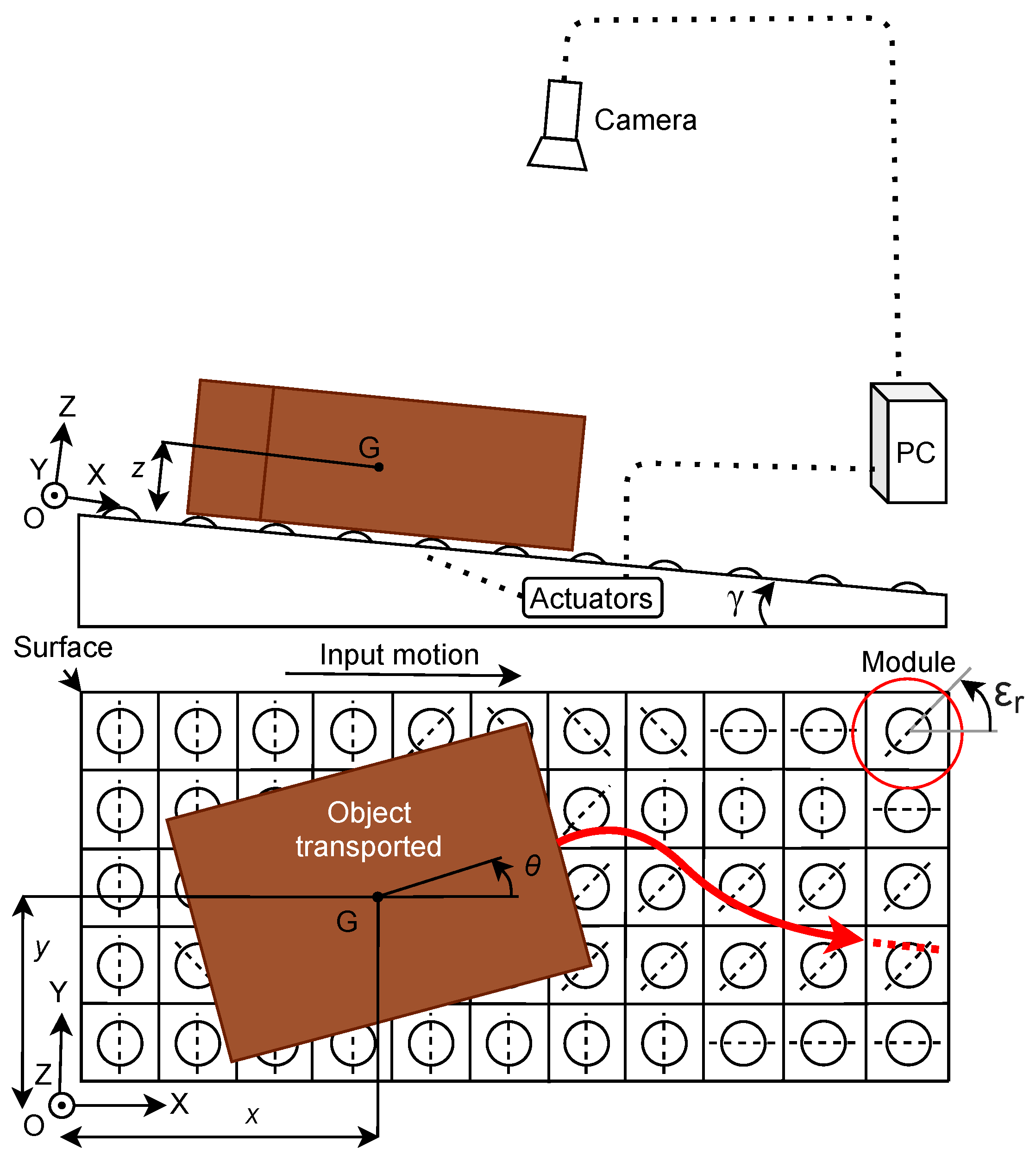
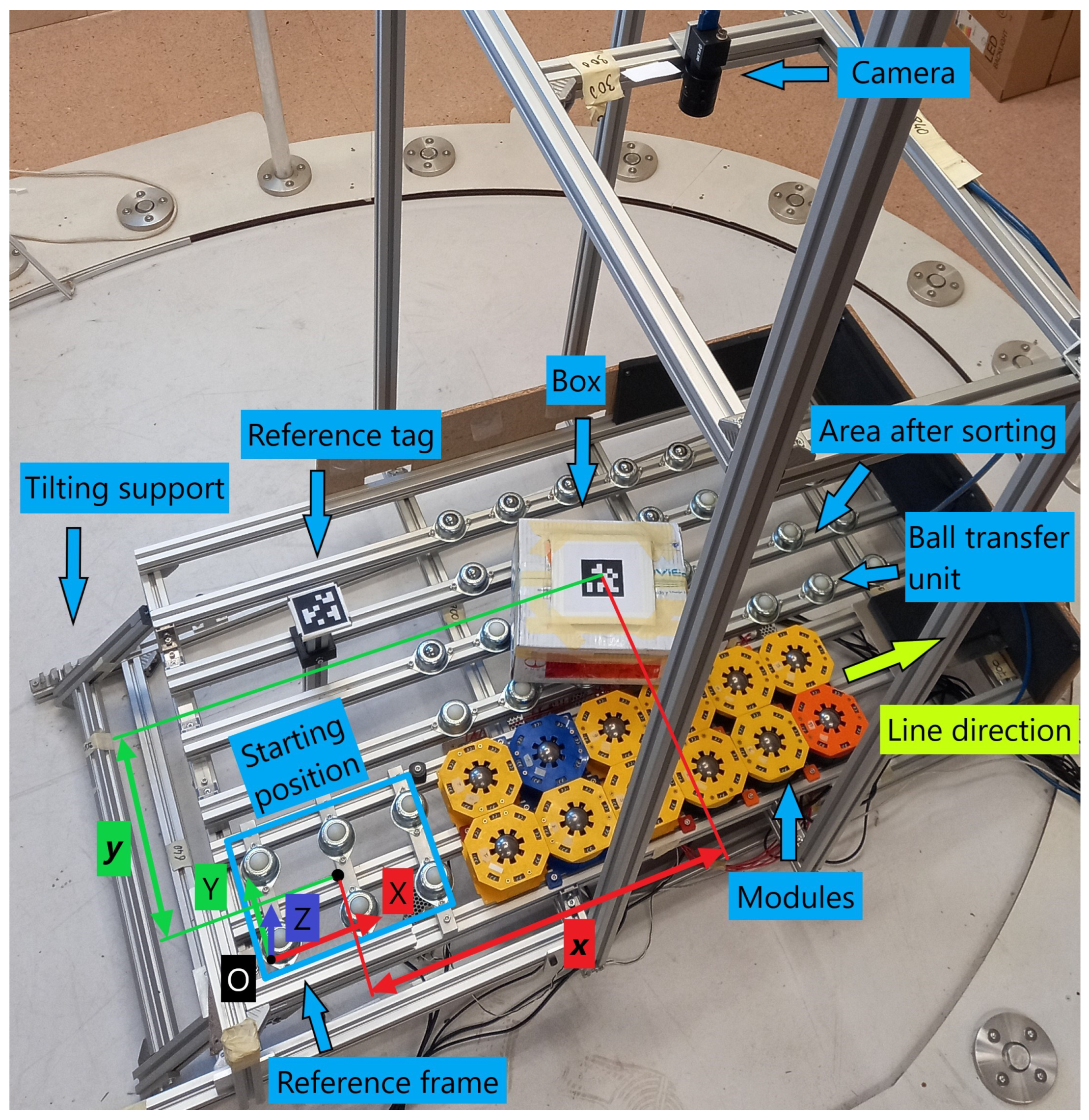
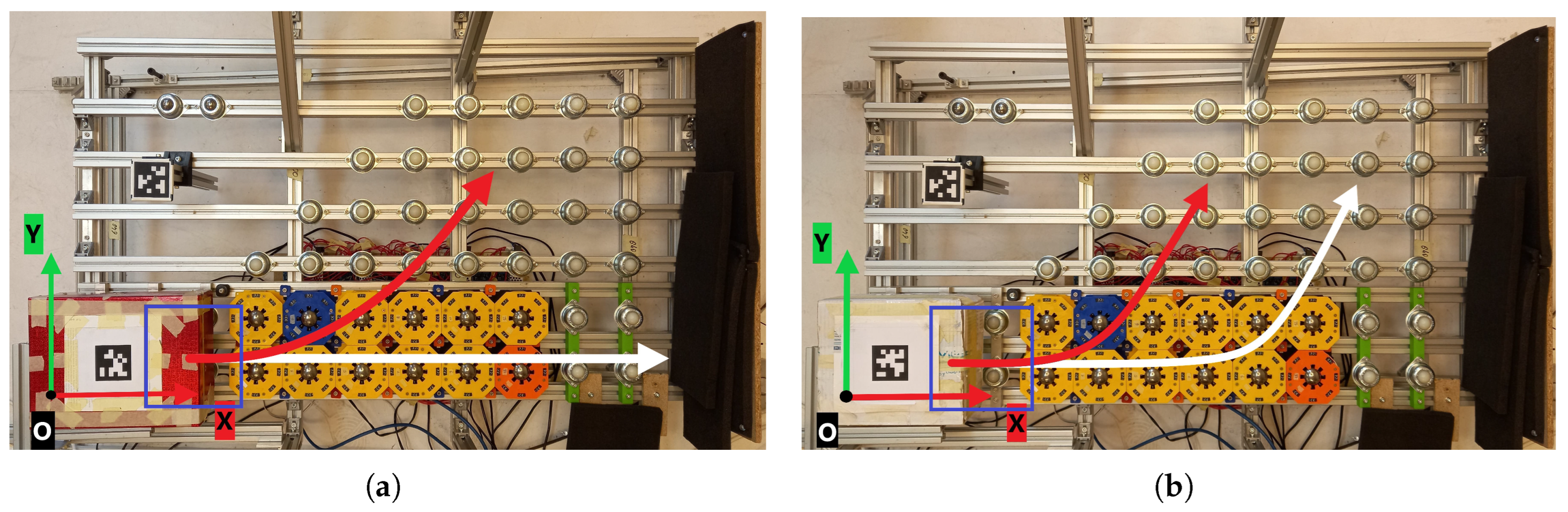
2.1. Physical Overview

The concept explored in this study involves an under-actuated modular surface, where each unit comprises an idle rotor whose swivelling axis direction (${\epsilon }_r$) in the surface plane can be controlled. A sphere serves as the material handling rotor (Figure 1), with its axis of rotation restricted to a few discrete orientations (${\epsilon }_r$: 0°, 90°, $\pm 45$°). This device utilizes passive rotors with orientable axes to generate a friction field capable of handling and manipulating the motion of packages. The absence of direct actuation for the transported material is compensated by leveraging gravity (e.g., tilting the surface), pre-existing input velocity (e.g., from a conveyor before the surface), or a combination of both. Further details about the specific design are provided in [2,19], while this paper introduces only the general functionality, focusing on the exploration of control strategies. Nonetheless, a physical prototype built to test the system’s functionality and the first control method (threshold-based, Section 3.1) is illustrated in Figure 2.

Similar to state-of-the-art solutions in the logistics industry [20], the proposed device includes a feedback system employing one or more cameras above the surface [15] (Figure 2), as seen in other in-plane handling technologies [1,17]. This sensor continuously processes frames of the working area to detect the position and other relevant information about the object handled in real time. Using this data, a processing unit (PC in Figure 1) connected to both the camera and the actuators (modules of the surface) is supposed to perform various handling tasks by applying appropriate control laws. With reference to the prototype surface shown in Figure 2, a FLIR Blackfly S Monochrome camera with 6.3 MP resolution and 59.6 fps is used as the sensor, while the processing unit includes a PC running Matlab (R2022b) for image analysis and an Arduino Mega for module actuation. In the illustrated setup, AprilTags [21] are applied to the object as fiducial markers for tracking and to the surface for reference. This approach allows the use of Matlab’s ReadAprilTag function to determine the tags’ poses and ID numbers. However, depending on the environment and task, other object detection strategies can also be applied.

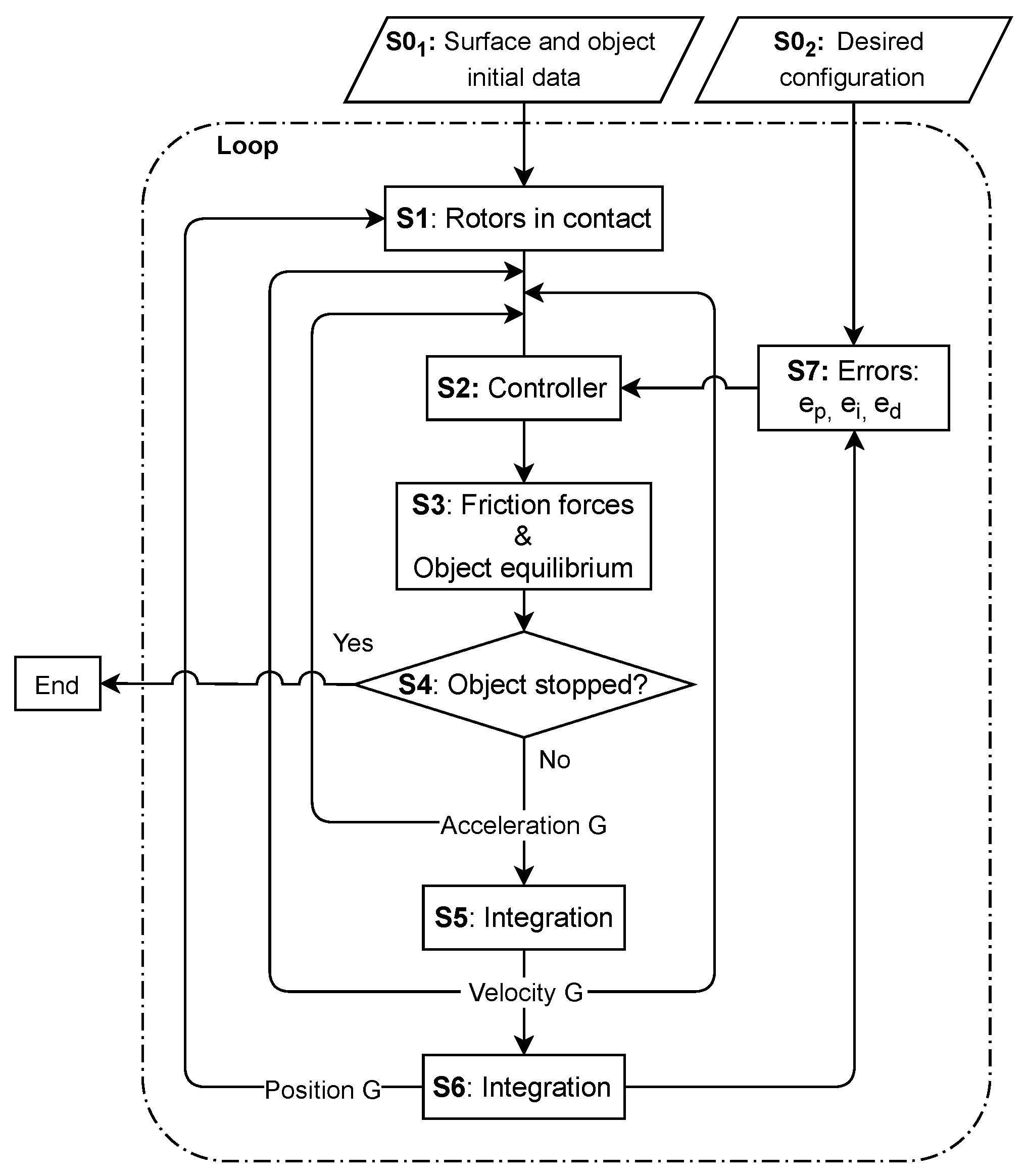
2.2. Software Overview

While the experimental setup shown in Figure 2 was used to test the so-called threshold-based control, the decentralized PID evaluation builds upon a previously established digital model developed to offer an efficient and cost-effective testing methodology. Beyond these advantages, including speed and versatility, the use of the simulation environment was also motivated by the limited sensing capabilities of the physical prototype, which would not allow for reliable PID testing at this preliminary stage. In [2], this digital model, designed to replicate a surface with specific physical characteristics, was introduced and experimentally validated. The software environment accurately simulates an object’s motion based on key input parameters, such as its geometry, mass, surface layout, and friction conditions. Furthermore, the demonstrated high accuracy of the model’s predictions in [2] reinforces its suitability for streamlining PID control analysis in the current study.

To give a brief introduction of this digital model, Figure 3 presents the logic scheme that was later implemented in Matlab and Simulink to describe the object’s motion on the under-actuated surface. Employing the flowchart in [2] and its representation style as reference, the diagram in Figure 3 incorporates additional terms related to control, including the desired configuration, errors, and the controller. In more detail, the steps followed by the controlled system are: $S{0}_1$, $S{0}_2$, $S1$, $S2$, $S3$, $S4$, $S5$, $S6$, and $S7$. The first two steps involve the implementation of the system input data: $S{0}_1$ pertains to the surface and the transported objects, while $S{0}_2$ addresses the desired configuration, which is the objective of the control. Step $S1$ focuses on determining the modules in contact, based on the object’s position. This position, along with velocity and acceleration data, and the errors derived from $S7$, are processed in step $S2$ by the control module. This step ($S2$) outputs the orientations of the module axes (${\epsilon }_r$), which are then used in step $S3$ to calculate the new friction forces and the body’s equilibrium. At this point, the stop condition is verified ($S4$). If the response is negative, the cycle continues with the integration of accelerations to velocities ($S5$) and then to position ($S6$). With this new information, the rotors in contact are determined again, and in step $S7$, the differences with the desired condition are calculated, thus the errors, along with their derivatives and integrals, and in this way the loop continues.

At this point, with the concept features and the model defined as above, the following sections illustrate the control strategies developed for the system. Specifically, the first control method, referred to as threshold-based, is explained and tested using the available physical setup of the surface. Conversely, the second method, which employs a PID controller and is designed for a system with these characteristics, is tested using the digital model of the surface, as introduced in this subsection.

3. Control Method

This section presents the control methodologies developed for the system. In the first subsection (Section 3.1), the threshold-based strategy is introduced and explained, while the second subsection (Section 3.2), focuses on the PID controller.

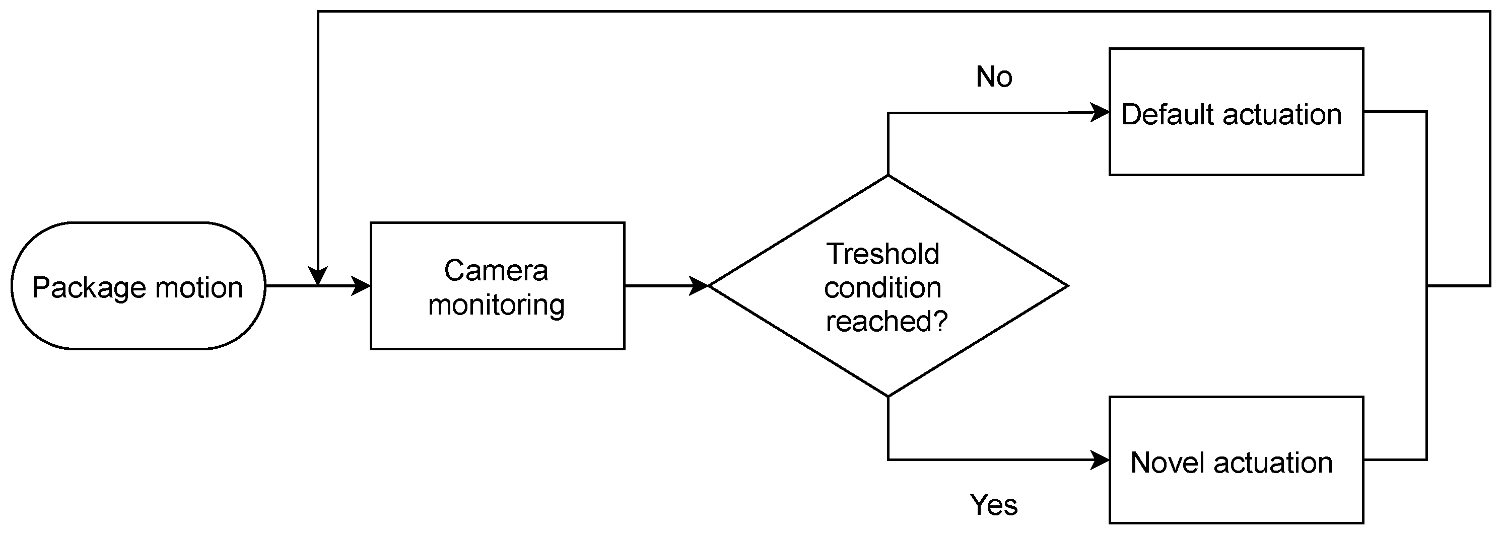
3.1. Threshold-Based Control

In scenarios where discrete, rule-based decisions are sufficient, the threshold-based control strategy offers an efficient way to trigger module actuation. It continuously monitors parcel features (such as identification markers) and activates the relevant module as soon as a preset condition is met (Figure 4), making it ideal for tasks like sorting and basic orientation. With reference to the experimental setup described in Section 2.1, a camera system captures images of the parcels as they travel along the surface. These images are processed in real time by a dedicated software environment, where a defined region of interest (ROI) is analyzed for markers, such as AprilTags, that identify each package. When a marker is detected and its identification code is retrieved, the control system compares the information against preset thresholds corresponding to the desired operation.

The selection of activated modules depends on both the final objective and the nature of the threshold condition met. Different types of thresholds can be defined. For instance, in one category of tests, the control system directs parcels along different trajectories using predefined module orientations based solely on their identifying IDs. In these tests, the threshold condition is simply the package’s “name.” In another set of experiments, the system is used for package reorientation. Here, the primary goal is to adjust the orientation of a parcel by specific angles as it passes through the smart surface. Consequently, in this case, the threshold variable is the angle, requiring more extensive and continuous monitoring.

In summary, threshold-based control for this technology relies on a real-time monitoring framework that couples image processing with targeted actuator commands. By tailoring the actuation logic to the specific task, whether diverting a parcel along a different path or re-orienting it by a defined angle, the method demonstrates a simple, yet versatile and robust approach for managing automated material handling processes. The subsequent sections will delve deeper into each application, providing further experimental insights and quantitative evaluations.

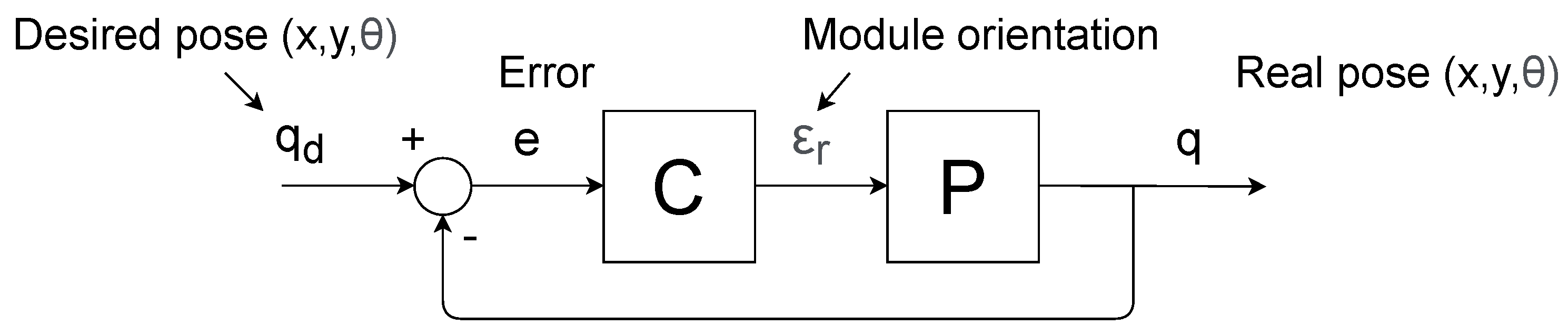
3.2. PID Control

For more demanding tasks such as precise position tracking, a refined control approach is required, one that continuously adjusts the control output in a progressive manner. The PID control strategy accomplishes this by constantly computing the error between the current and the desired position and generating a control signal composed of proportional, integral, and derivative components. Supported by various studies in the literature (e.g., [1,11]), this method was selected as the second control strategy for the technology under investigation to tackle more complex handling operations even under challenging conditions.

Even though PID control is a simple and widely used control method, its definition and implementation are not straightforward, as the logic must be tailored to the system’s specific features and operation. This section explains the formulation and underlying principles of the control approach. The analyzed system is quite complex in its control description. Firstly, the constraints linking the object to the surface vary over time (holonomic constraints) and are generally redundant. For example, depending on the pose, the object can be on 4, 5, or 6 modules (at least the boxes employed in the following tests), requiring the use of minimization algorithms to calculate the distribution of contact forces [14], thus introducing significant nonlinearities. Secondly, the surface is an under-actuated system, meaning it does not use driving forces for movement but rather friction ones that tend to stop the transported material. For example, the material flow can only be in the direction of the line, and reverse motion is not possible [14]. This feature limits the handling capability and necessitates the use of a specific friction model tailored to the concept design [12]. Thirdly, the regulation of actuation forces is not continuous but discrete, as the axes can be positioned in only a few predefined directions. This, like the redundancy of the contact points, necessitates minimization functions to calculate which discrete position produces the lowest errors. As an additional note regarding the contact force, the minimization algorithm was preferred over other studied methods, such as the spring-contact model in [15], because it prevents unrealistic negative solutions.

Because of these complexities, it is not possible to define direct or inverse kinematics for the system, as is done with a serial manipulator or when the rotor velocity is controlled [1,11], nor is there a simple or explicit rule associating the desired body configuration with the orientations of the axes. The power dissipation method (PDM) must also be excluded for the dynamic description, as the system does not operate under quasi-static conditions [17]. A more reasonable approach is to use dynamic control by implementing tailored contact and friction models [14,19], and subsequently utilizing the equations of motion to determine the orientation of the module axes. In fact, it appears feasible to numerically identify the combination of axis orientations that provide the necessary forces for the desired acceleration, and consequently, for velocity and position. The procedure for achieving this is presented below, along with the formulations employed.

From the Lagrangian, the vector representation of the dynamic equations of an object in equilibrium on the surface [14] can be written as:

$$B\left(q\right)\ddot{q}+C(q,\dot{q})\dot{q}+G\left(q\right)=Q(q,\dot{q})$$

(1)

where $q=[x_g,y_g,{\theta }_g]$ is the vector that contains the variables that describe the configuration of the system (in the surface reference frame, as shown in Figure 1). In particular, since $z_g$ is not changing in the reference frame that is fixed on the tilted surface, q does not include it. Q consists of generalized forces and torques acting on the system, C is the Coriolis matrix, G is the vector of gravitational contributions, and B is the dynamic inertia matrix, which in this instance is independent of q. These concepts are specifically defined using the nomenclature used in [14]:

$$B=\left[\begin{array}{ccc}m& 0& 0\\ 0& m& 0\\ 0& 0& J\end{array}\right]C=\left[\begin{array}{ccc}0& 0& 0\\ 0& 0& 0\\ 0& 0& 0\end{array}\right]G=\left[\begin{array}{c}-mgsin\left(\gamma \right)\\ 0\\ 0\end{array}\right]$$

$$Q=\left[\begin{array}{c}\sum _{i=1}^{n_i}{F}_{x_i}\left({\epsilon }_{r_i}\right)\\ \sum _{i=1}^{n_i}{F}_{y_i}\left({\epsilon }_{r_i}\right)\\ \sum _{i=1}^{n_i}(x_{GP}{F}_{y_i}\left({\epsilon }_{r_i}\right)-y_{GP}{F}_{x_i}\left({\epsilon }_{r_i}\right))\end{array}\right]$$

Achieving the desired configuration $q_d$, which may change over time (trajectory) or stay constant (position), is the aim of control. Equation (2) expresses the intended generalized forces and torques in PID control [23]. This ideal configuration, along with the actual configuration q, defines the error term $e=q_d-q$.

$$Q_d(q,\dot{q})=K_p{e}_p+K_i{e}_i+K_d{e}_d+G$$

(2)

In this case, the terms are the following. First, $e_p$, which coincides with e, is the proportional error term with its coefficient matrix $K_p$. Secondly, $e_i$ is the integral term $e_i={\int }_0^{t}e\left(t\right)dt$ with its coefficient matrix $K_i$. Thirdly, $e_d$ is the derivative term, denoted as $e_d={\displaystyle \frac{de\left(t\right)}{dt}}$ with its related matrix, $K_d$. Ultimately, G employed to compensate the gravitational term. The Lyapunov candidate of the system $(V={\displaystyle \frac{1}{2}}{e}_d^{T}B{e}_d+{\displaystyle \frac{1}{2}}{e}_p^T{K}_p{e}_p)$ should ideally trend to zero given these forces and the $q_d$ constant, guaranteeing system stability.

Nevertheless, these forces are not generated by modules that are completely actuated and capable of orienting in every direction. Therefore, at this stage of the process, the objective is to find a combination of orientations for the module axes that minimizes the norm of the difference between the ideal and actual force values (Equation (3)).

In practice, all possible k-permutations are taken into consideration because each module can only be oriented in four different ways (${\epsilon }_r$: 0°, $\pm 45$°, 90°) plus the free sphere condition (${\epsilon }_r$: none; the blocked case was not included), and there are typically few modules in contact (less than ten, for instance). As stated before, for every permutation, the difference with $Q_d$, the difference that is really produced Q, and the norm of this difference are computed. Next, using Equation (3), the set of angles (${\epsilon }_{r_i}$) that yield the smallest norm is chosen. As a result, oscillations around the intended configuration are caused by intrinsic disturbances in the system. Although these variances cannot be completely eliminated, they can be minimized by speeding up the system’s reaction and analysis times.

$${\epsilon }_r:min\{Q_d-Q\}$$

(3)

Figure 5 presents a flowchart summarizing the control scheme that implements the aforementioned logic. In addition to the previously defined terms, C represents the control block, while P denotes the system dynamics. This concludes the introduction to the theoretical aspects of the applied controls. In the following subsections, experimental and simulated results obtained from applying the threshold-based and PID controllers will be presented.

4. Results

This section is focused on reporting the experimental results obtained for the threshold-based method in Section 4.1, and the simulated outcomes of the PID controller in Section 4.2.

4.1. Threshold-Based—Experimental Results

As previously introduced, the setup built and reported in Figure 2 was employed to test the actual functioning of the threshold-based method. Practically, two common intralogistic operations, i.e., sorting and orientation, were selected as handling tasks for the system control experimental validation. In the first case, the threshold condition was the ID of the package, while in the second case, the orientation angle was the controlled variable. These two operation outputs are presented in the following subsections.

4.1.1. Sorting Results

Two primary testable setups, designated CS1 and CS2, were developed in this preliminary sorting study employing the given surface. Both of the proposed experiments are displayed in Figure 6. Specifically, Figure 6a introduces CS1, where the two packages with different AprilTags, i.e., Box A (white box) with ID = 1 and Box B (red box) with ID = 0, are, respectively, meant to pass straight on, or to be sorted to the left. In the figure, only the red package, Box B, is reported, but the different coloured arrows indicate the intended paths of the two boxes: red arrow = Box B (red), white arrow = Box A (white). The same applies to Figure 6b, illustrating CS2, where only Box A (white) is depicted, but both arrows are shown. In CS2 (Figure 6b), both packages are meant to be sorted, but at different stages along the line of modules: Box B is sorted early, while Box A is sorted afterward.

The control mechanism used to apply these types of sorting works as follows: The camera, operating at its own frequency (59.6 fps), sends the captured frames to Matlab. For each frame, a region of interest (ROI: blue square in Figure 6) located after the starting position of the package and before the actuating modules is analyzed in Matlab. In this ROI, Matlab continuously looks for a tag using the ReadAprilTag function. The signal (an integer) to be delivered via the serial port to Arduino, which will activate the preset modules for the intended task, is decided by the tag’s ID if one is available. Specifically, for CS1, with ID = 0 (Box B), the modules are all oriented with axes at 135°, while with ID = 1 (Box A), they are at 90°. In the case of CS2, with ID = 0 (Box B), the modules are all oriented with axes at 135°, whereas with ID = 1 (Box A), only the last 6 modules (the last 3 columns on the right side in Figure 6) along the line are oriented at 135°. These angular values define the rotor axis’s orientation from this point on. Measurements are made counterclockwise, beginning with the x axis in Figure 6. In addition to the box types, the following tests with the surface setup have the mass of the box (m = 7.5 kg) and the surface inclination ($\gamma$ = 8°) as input conditions. To evaluate the system’s response readiness, even with packages already in motion, an ROI that lies halfway between the initial location and the modules was selected.

As supplementary data,

Table 1. Times during the actuation resulting from 30 sorting operations, 15 for CS1 and 15 for CS2 [22].

	tm1 [s]		tm2 [s]		tm3 [s]		tm4 [s]
	$\mathit{\mu }$	$\mathit{\sigma }$	$\mathit{\mu }$	$\mathit{\sigma }$	$\mathit{\mu }$	$\mathit{\sigma }$	$\mathit{\mu }$	$\mathit{\sigma }$
Box A	$0.118$	$0.004$	$0.144$	$0.005$	$0.016$	$0.005$	$0.165$	$0.007$
Box B	$0.117$	$0.002$	$0.143$	$0.002$	$0.015$	$0.006$	$0.160$	$0.006$

shows the timing of the different recognition and actuation phases. As illustrated in Figure 4, the reaction times obtained depend on the stated system, its connections, and communication.

More in detail, in Table 1, the following terms are reported: tm1 is the time Matlab requires to access a frame from the camera, i.e., the time needed to take a picture using the Matlab function getsnapshot. tm2 is the time required for tm1 plus the image processing time, which includes correcting image distortions (using the undistortImage function), cropping the ROI (using the imcrop function), and detecting and reading the tag (using the readAprilTag function). tm3 is the time taken to send an integer value from Matlab to Arduino via the serial port and receive a response (also an integer via the same port) after executing the actuation command. The response from Arduino is not necessary, but it was used to estimate the actuation time. Finally, tm4 describes the total time that elapses from immediately before the image is captured to the moment Matlab receives the actuation response from Arduino. This is not precisely the total of the earlier times since it contains extra values associated with the code and, in particular, the tic and toc functions that Matlab uses to estimate the timings.

The camera’s maximum frame rate is 59.6 fps, which translates to one picture every 1/59.6 = 0.0168 s. Nevertheless, taking into account tm4 from Table 1, each frame is processed in roughly 0.16 s, which is roughly ten times longer. As a result, several optimization techniques (in this case, minimization) were taken into consideration after this preliminary assessment of the system’s response times.

In practice, tests were repeated with the goal of minimizing the most important processing time, which is tm1 as indicated in Table 1. As a result, the camera’s ROI was set to the value that was used in the imcrop function; in other words, the imcrop function is no longer necessary because the camera now only gives photos of the ROI.

Furthermore, the image distortion correction (the undistortImage function) was removed, and the videoinput (Matlab function) object setting was switched to manual triggering, following the suggestions presented in [24] to minimize the execution time of the getsnapshot function.

Table 2. Times during the actuation after optimization resulting from 30 sorting operations, 15 for CS1 and 15 for CS2 [22].

	tm1 [s]		tm2 [s]		tm3 [s]		tm4 [s]
	$\mathit{\mu }$	$\mathit{\sigma }$	$\mathit{\mu }$	$\mathit{\sigma }$	$\mathit{\mu }$	$\mathit{\sigma }$	$\mathit{\mu }$	$\mathit{\sigma }$
Box A	$4.70\times {10}^{-4}$	$6.96\times {10}^{-5}$	$1.94\times {10}^{-2}$	$1.64\times {10}^{-3}$	$1.44\times {10}^{-2}$	$5.49\times {10}^{-3}$	$4.05\times {10}^{-2}$	$7.75\times {10}^{-3}$
Box B	$4.31\times {10}^{-4}$	$1.96\times {10}^{-5}$	$1.83\times {10}^{-2}$	$5.96\times {10}^{-4}$	$1.26\times {10}^{-2}$	$5.42\times {10}^{-3}$	$3.57\times {10}^{-2}$	$6.10\times {10}^{-3}$

reports the resulting times with these adjustments. It is possible to observe a reduction in tm1 by a factor of 1000 and a reduction in the total time tm4 by a factor of 10, which brings it closer to the optimal maximum values permitted by the camera’s frame rate.

Returning to the actual sorting for the different cases and package types, Figure 7 displays the trajectories for case CS1, and Figure 8 displays the trajectories for case CS2. More precisely, the AprilTag’s contour is indicated in red, and the locations and paths of the tag’s center are indicated by circular markers and continuous green lines, respectively. Beginning with the first case CS1, it can be seen that Box A proceeds straight in Figure 7a, while Box B performs the sorting immediately in Figure 7b. On the other hand, for the second case, CS2, Figure 8a shows the sorting at the end of the line for Box A, while it happens at the beginning of the line for Box B, as in Figure 8b. The efficacy of this control for the examined tasks is demonstrated by these two images, which highlight agreement between the intended sorting results (Figure 6) and the actual ones.

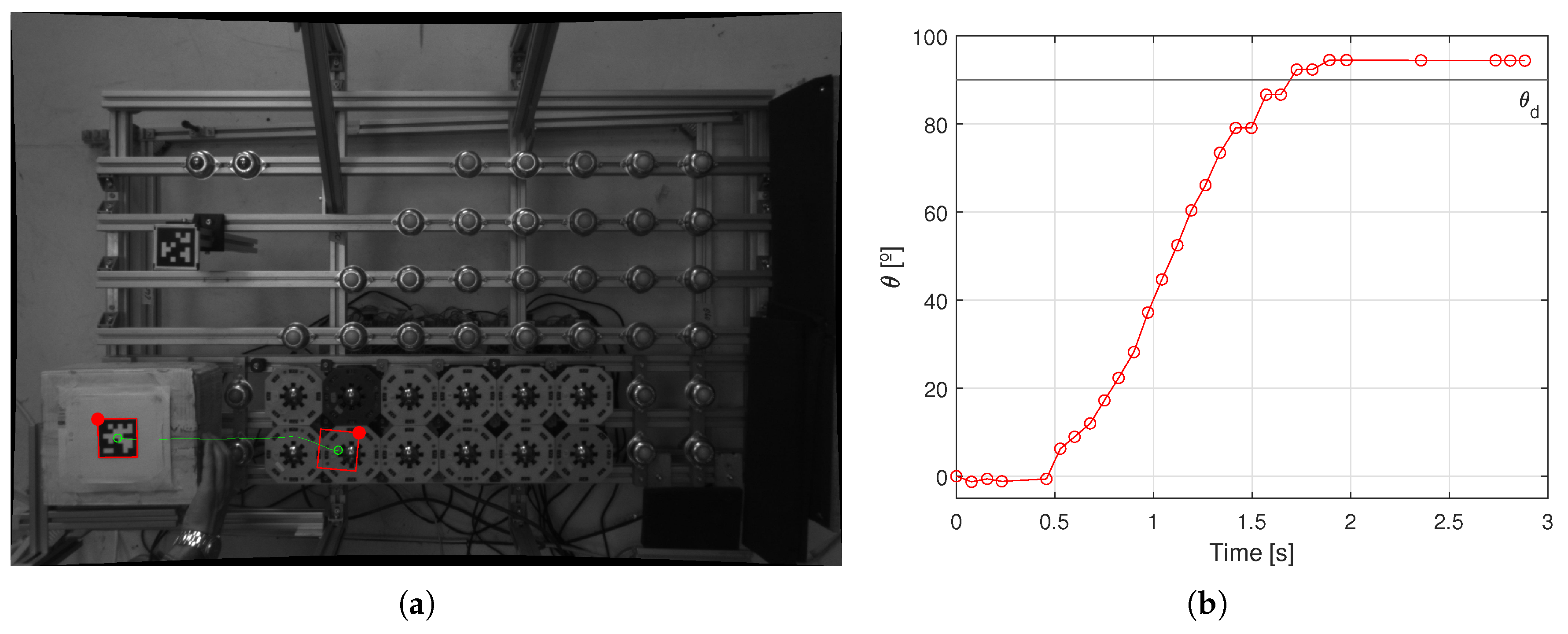
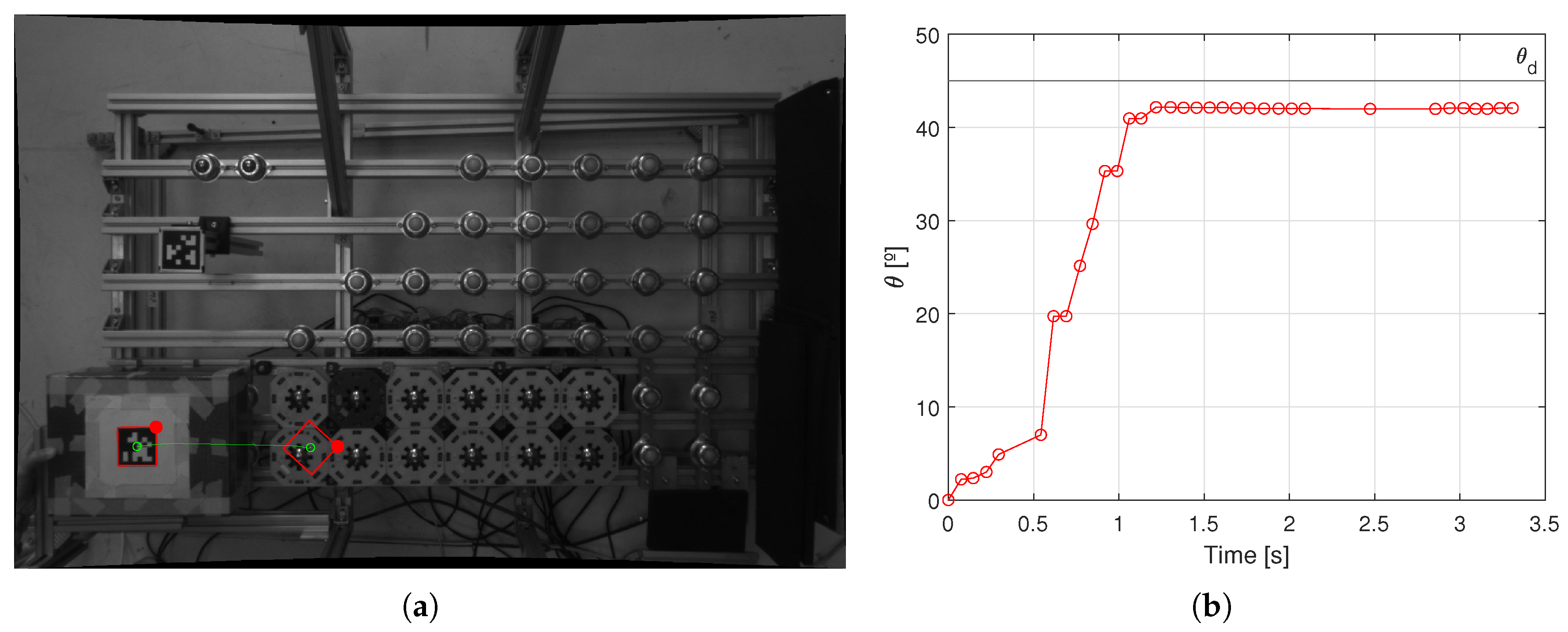
4.1.2. Orientation Results

Another task that seemed interesting to test with the setup is the orientation of packages. As examples of the system’s application, slightly different tests were carried out based on the type of Box, while the mass and the inclination inputs remained the same ($\gamma$ = 8°, m = 7.5 kg). The package was supposed to be reoriented by $\theta$ = 90° for Box A and by $\theta$ = 45° for Box B. The way the modules are arranged differs from the assignments that have been shown so far. In the earlier testing, the changes were always made by columns, meaning that one column or a group of columns was different from the rest, assuming that the layout consists of two rows and six columns of modules. On the other hand, in this case, the modules’ orientation differs by row. In actual use, the modules of the lower row (Figure 9) had their axis parallel to the line (0°) activated for the packages to rotate (clockwise in the tests recorded), while the top ones remained free. This makes sure that the package on the inclined surface comes into contact with areas of increased friction, which serve as pivots and allow for easier rotation around them. As soon as the package enters the designated ROI, tag monitoring begins, and therefore sorting. Here, the orientation variation is tracked by looking at the line that connects the tag’s two corners and how its orientation varies with respect to the x axis once the tag’s ID has been distinguished. When the angle reaches, frame by frame, the desired value, the system simultaneously blocks two axes of the free row modules plus the 90° axis of the already actuated row ones, so that all the spheres are blocked and the orientation stops. The speed ($\dot{\theta }$), angular acceleration ($\ddot{\theta }$) and the time elapsed per frame ($t_f\simeq$tm4, without the message back Arduino-Matlab) are also included in the angle estimation, which, considering the initial orientation value as 0, is $\theta ={\theta }_0+\dot{\theta }·t_f+0.5·\ddot{\theta }·t_f^2$ (to anticipate the next iteration).

Figure 9a and Figure 10a illustrate the poses of the tags and the trajectories taken with the same markers and colors as the previous operations outcomes. For this case, an extra red circular marker was added to one corner of the tag to graphically clarify the magnitude and direction of the rotation. For the quantitative depiction, Figure 9b and Figure 10b describe the desired angle ${\theta }_d$ and the trend of the angle $\theta$ over time, respectively, for Box A and Box B. As seen from both pairs of images, the re-orientations are accomplished with minimal margins of error, i.e., $\theta =94$° instead of ${\theta }_d=90$° and $\theta =43$° instead of ${\theta }_d=45$° (both relative percentage errors: $4.4$%). The values in the examples appear reasonable when taking into account the uses for these surface capabilities. The orientation along the line might, in fact, optimize palletizing or later re-handling operations that do not require extremely precise positioning while shipping packages or transporting materials.

In summary, both the sorting and orientation operations employ a unified threshold-based control framework triggered by AprilTag detection, yet they differ fundamentally in actuation logic and feedback integration. The sorting task implements an on–off control scheme: upon tag ID recognition within the ROI, a discrete column-wise reorientation command is issued, without further continuous feedback. In contrast, the orientation task adopts a hybrid threshold-plus-feedback strategy, continuously estimating the package’s angular state and actuating or locking entire module rows once the setpoint threshold is crossed, following a predictive on–off logic informed by angular velocity and acceleration.

This comparative analysis highlights the capacity of the same under-actuated modular surface, equipped with minimal sensing and discrete actuation, to realize both discontinuous and quasi-continuous control strategies. Such versatility underscores the platform’s robustness and adaptability, demonstrating its suitability for a range of intralogistics tasks under a common control paradigm.

4.2. PID—Simulated Results

As previously stated, the analyses and tests of the decentralized PID control operation and performances were conducted employing the surface digital model summarized above and extensively explained in [2,14]. Specifically, two main industrial cases were investigated and simulated: a sorting system with four aligned outputs (PATH 1) and one with outputs on both sides of the transport line (PATH 2).

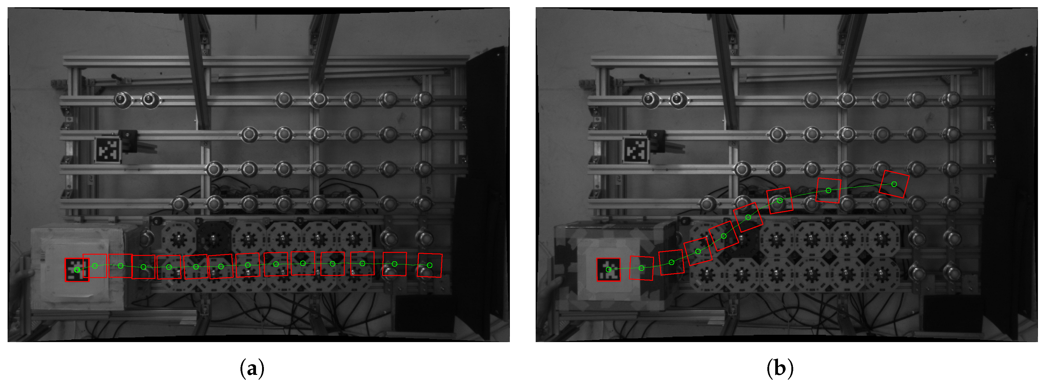
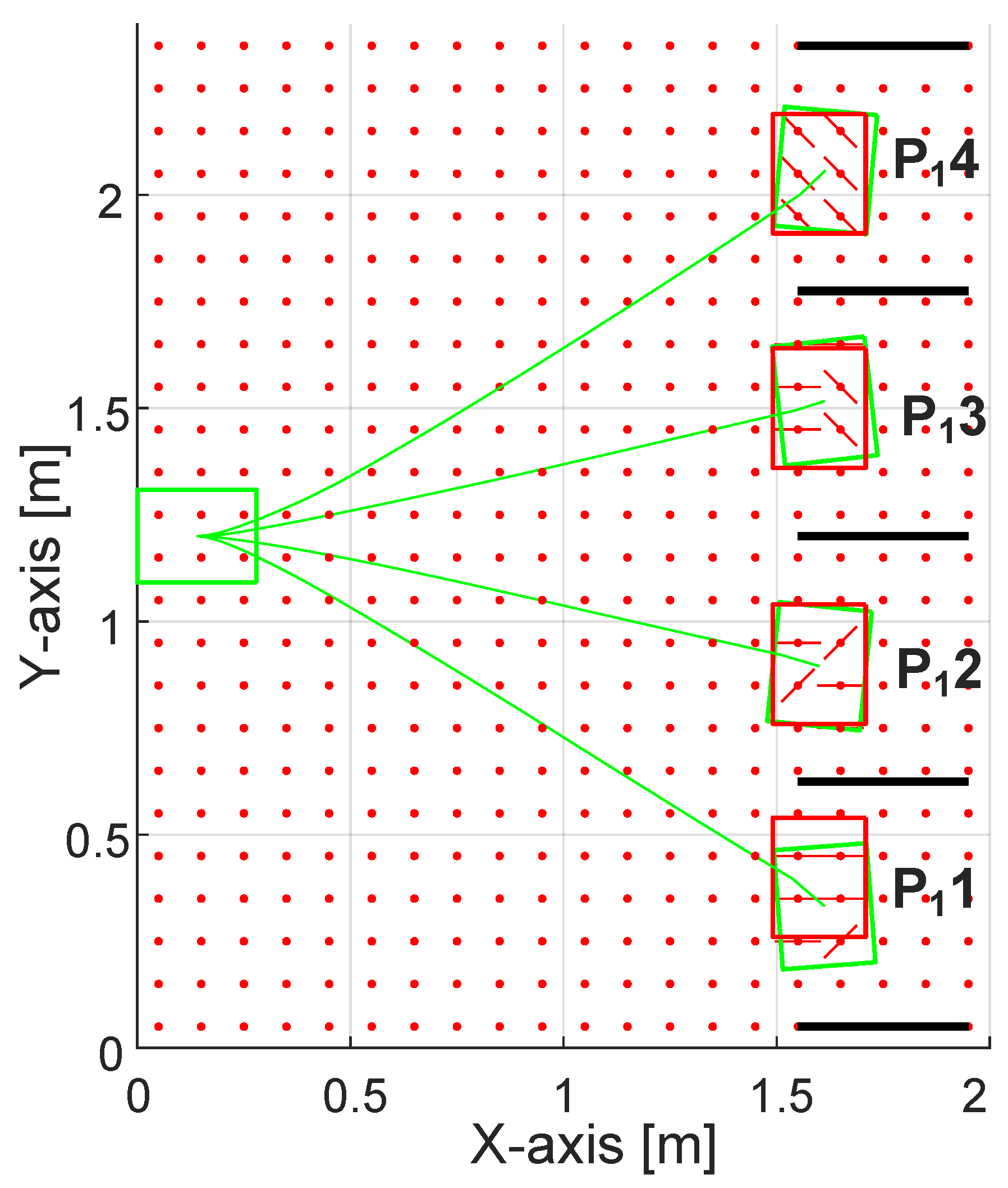
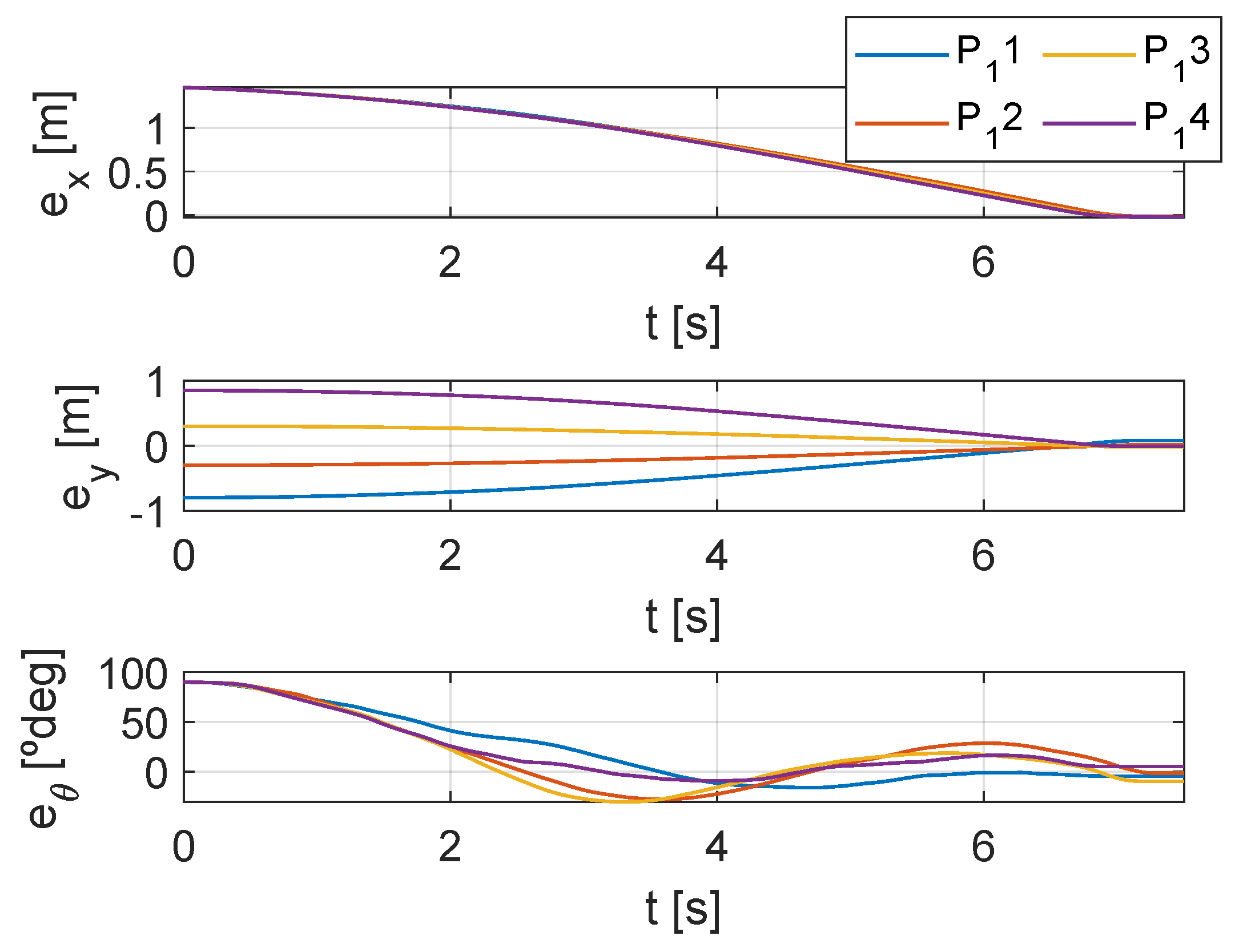
Results PATH 1

An “end of the line” sorting scenario with four outputs was selected for the initial simulation of a possible use. This task emerged after a discussion with the industrial partner Dumarey Flowmotion Technology, during a research stay at the company. Practically, they had a line with four final codes that needed to be separated into different slots to speed up and simplify palletization with a cobot (Figure 11).

The industrial specifications required for a similar application, which in this case were provided by the company, are the number of outputs (4), their arrangement (in line as in Figure 11), the maximum footprint available (2 m × 2 m), the parcel transported (Cardboard box: length width and height, 0.28 m × 0.22 m × 0.1 m, mass 7.5 kg), and its initial and final position (as in Figure 11). In line with these terms, the test was designed by defining the layout, the surface characteristics, and the package features. Figure 12 presents the graphical results of the simulations, and the chosen layout is also visible. While the green lines in the image represent the center of mass (COM) trajectories for the different simulations, each of which ends in a green rectangle of its final configuration, the green rectangle on the left depicts the package in its initial position, where it has virtually no speed (0.05 m/s in the x direction). The under-actuated modules are responsible for the movement and reorientation towards the slots (spaces between the black lines), while the inclination of the surface (8°) causes the motion towards $x>0$. The red dots in the figure represent the module rotors. They are in a free-sphere state at that time if they are not accompanied by intersecting lines that denote their rotation axes. The target positions in the different simulations are indicated by the red rectangles, while the actuated axes are only visible in the final arrangement. Although only the axes of the modules in the final condition are shown for graphical clarity, what actually happens is a continuous reorientation of these axes as the box passes over. The calculation and implementation of the actuation take place at each discrete time period (0.01 s for the described simulations). The module returns to the state of an unpowered free sphere once it is no longer beneath the object. Thus, even though they have pushed the material in the direction of the targets, the spheres in the center of the image are all free. Figure 12 shows that the desired positions (called: $P_{1}1$, $P_{1}2$, $P_{1}3$ and $P_{1}4$) are reached in all four cases, with adequate precision for the intended purpose. To quantify these values, the error trends for the various configurations are also reported (Figure 13). Figure 13 illustrates how the errors tend to zero with different oscillation levels. The required times for the selected parameters are also visible. On this matter,

Table 3. Settling time ($St$) with 2% threshold for the two displacements x, y and the orientation $\theta$ in the four outputs cases of PATH1.

	${\mathit{S}\mathit{t}}_{\mathit{x}}$ [s]	${\mathit{S}\mathit{t}}_{\mathit{y}}$ [s]	${\mathit{S}\mathit{t}}_{\mathit{\theta }}$ [s]
$P_{1}1$	$7.176$	$7.134$	$6.931$
$P_{1}2$	$7.228$	$7.194$	$7.255$
$P_{1}3$	$7.135$	$7.086$	$7.133$
$P_{1}4$	$7.080$	$7.079$	$6.842$

introduces a standardized metric, i.e., the settling time, for further comparison among the four position tracking tasks, but also with PATH2 and other control methods once developed. These times are calculated considering the threshold of 2% around the desired equilibrium condition. The values resulting from this table indicate that the parcels settle around the equilibrium just a few instants before the simulation end, pointing out a halting condition that occurs near the ideal outcome.

The initial controller coefficients $K_p$, $K_i$, and $K_d$ were manually adjusted to obtain a stable response and define a reasonable starting point for the optimization phase. These preliminary values were then refined using the particleswarm function in MATLAB R2022b, MathWorks, Natick, MA, USA, which was employed to simultaneously minimize the final position errors across the four different scenarios with respect to their respective targets. Specifically, the objective function was defined as the total IAE (Integral Absolute Error), computed by summing the IAEs (each one discretized as ${\sum }_{i=1}^n\left(e_{x_i/y_i/z_i}\right)$) over all four scenarios [25,26]. Following preliminary tests, the particleswarm method was preferred over fmincon [25] due to its higher efficiency in finding globally optimal solutions, as also discussed in [27] for another smart handling system.

To ensure feasibility in terms of computation time, the optimization was performed with a swarm size of 20 and 20 iterations. The parameter bounds were restricted within reasonable physical limits, with each of the controller gains $K_p$, $K_i$, and $K_d$ limited to values between 0 and 100.

Furthermore, simplified control strategies were tested by zeroing out specific gain matrices. Setting $K_i=0$ led to a PD controller, while setting $K_d=0$ resulted in a PI controller. These configurations produced inferior performance in terms of final error and stability compared to the full PID controller, which was ultimately selected and reported in this analysis.

The optimized PID gains used in the simulations (with a maximum duration of 7.5 s) are as follows:

$$K_p=\left[\begin{array}{ccc}0.2957& 0& 0\\ 0& 0.3950& 0\\ 0& 0& 0.1827\end{array}\right]K_i=\left[\begin{array}{ccc}0.0059& 0& 0\\ 0& 0.0088& 0\\ 0& 0& 0.0094\end{array}\right]K_d=\left[\begin{array}{ccc}0.0532& 0& 0\\ 0& 0.0502& 0\\ 0& 0& 0.1278\end{array}\right]$$

Although some oscillatory behavior remains due to the inherent under-actuation and instability of the system (see Section 3.2), the results are acceptable for the intended applications and robust across different layouts, materials, and inputs. Future studies may further refine these parameters for specific operating conditions. In summary, the control system effectively finished the tasks in compliance with the company’s and industry’s requirements. Consequently, the solution will be taken into consideration for a future real implementation.

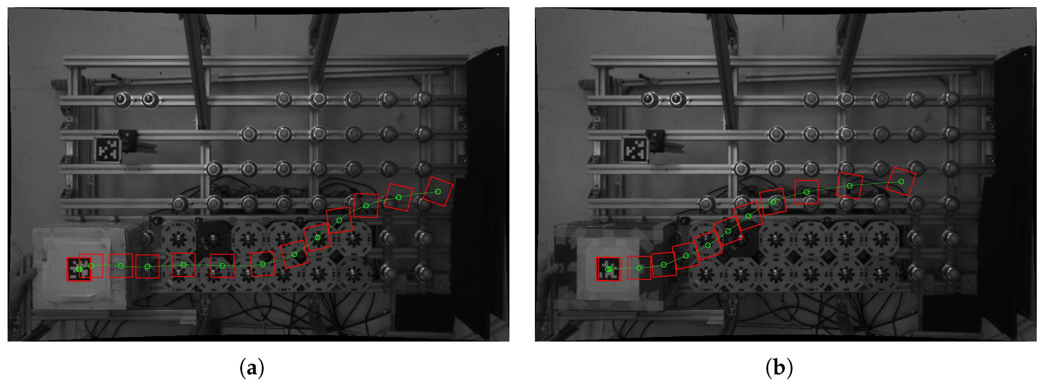
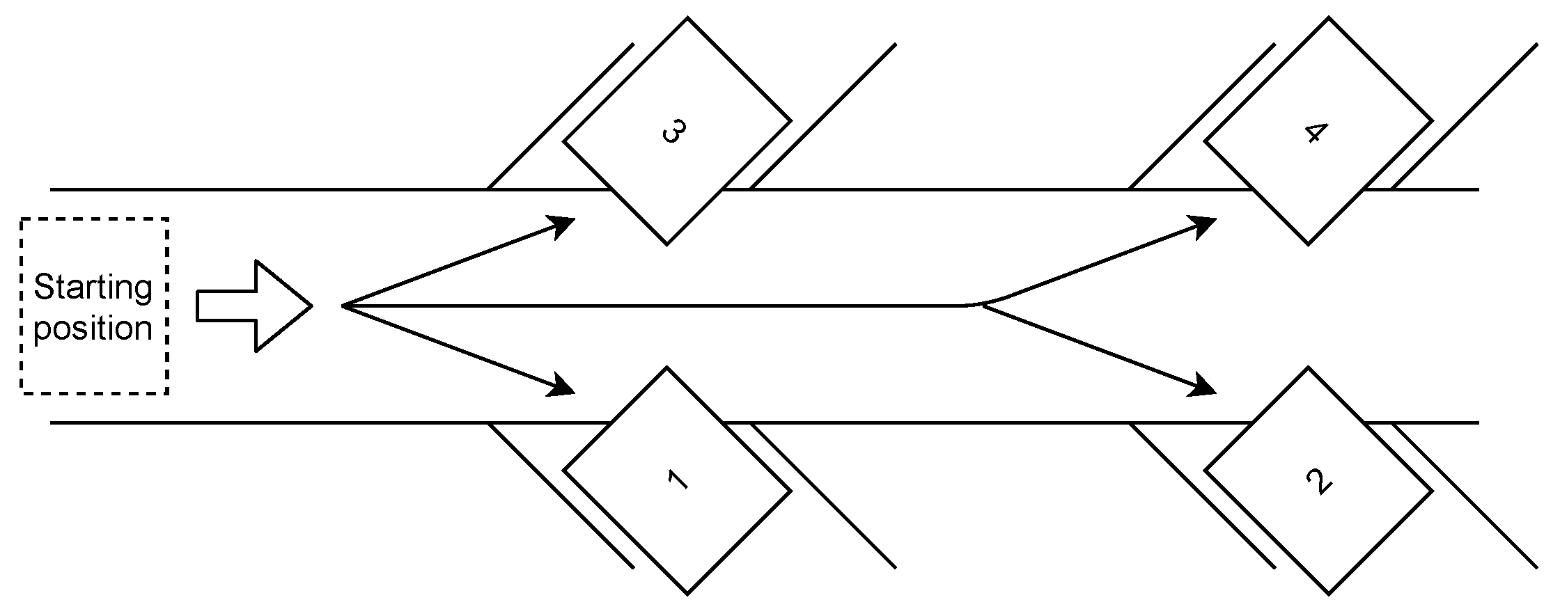
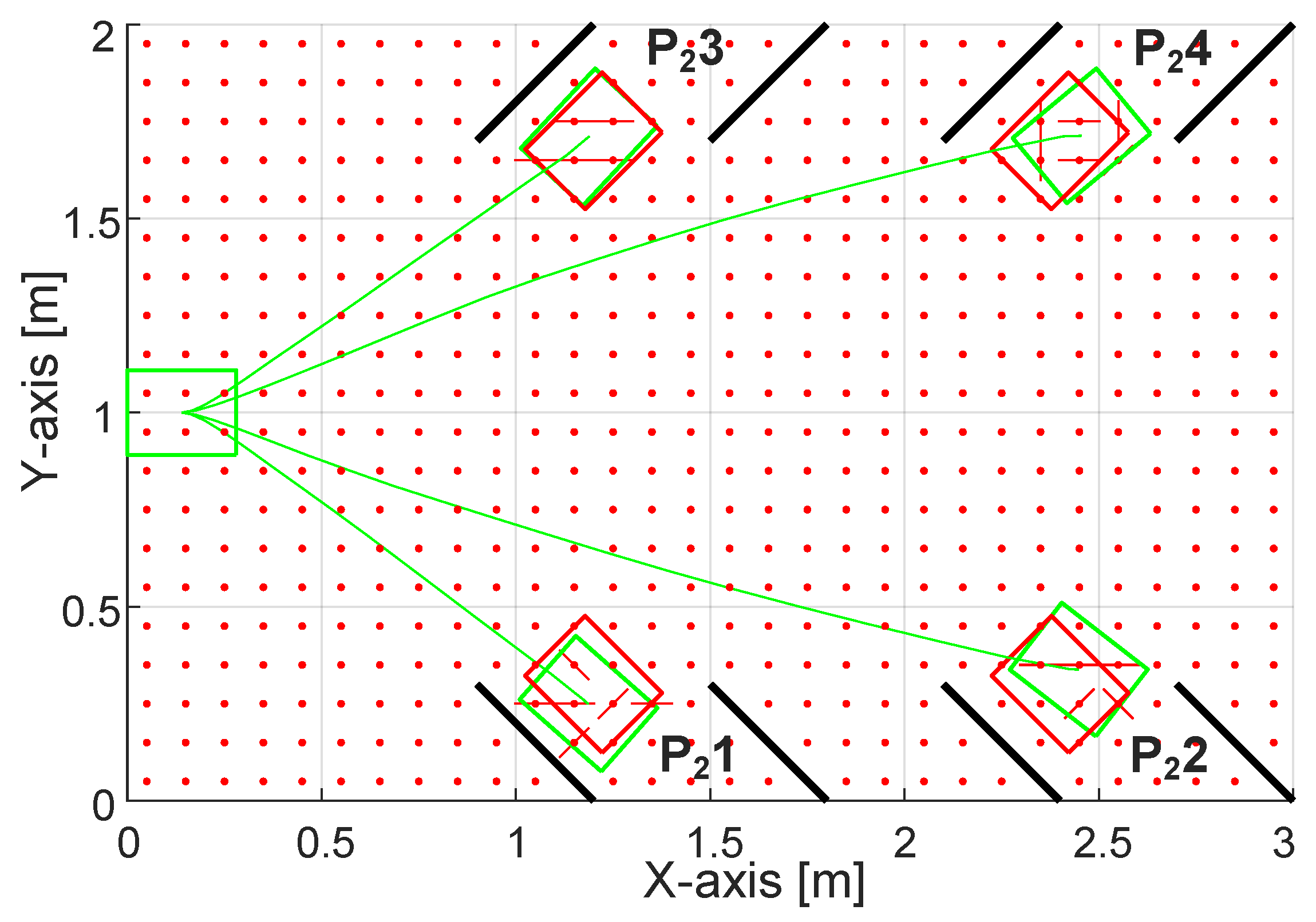
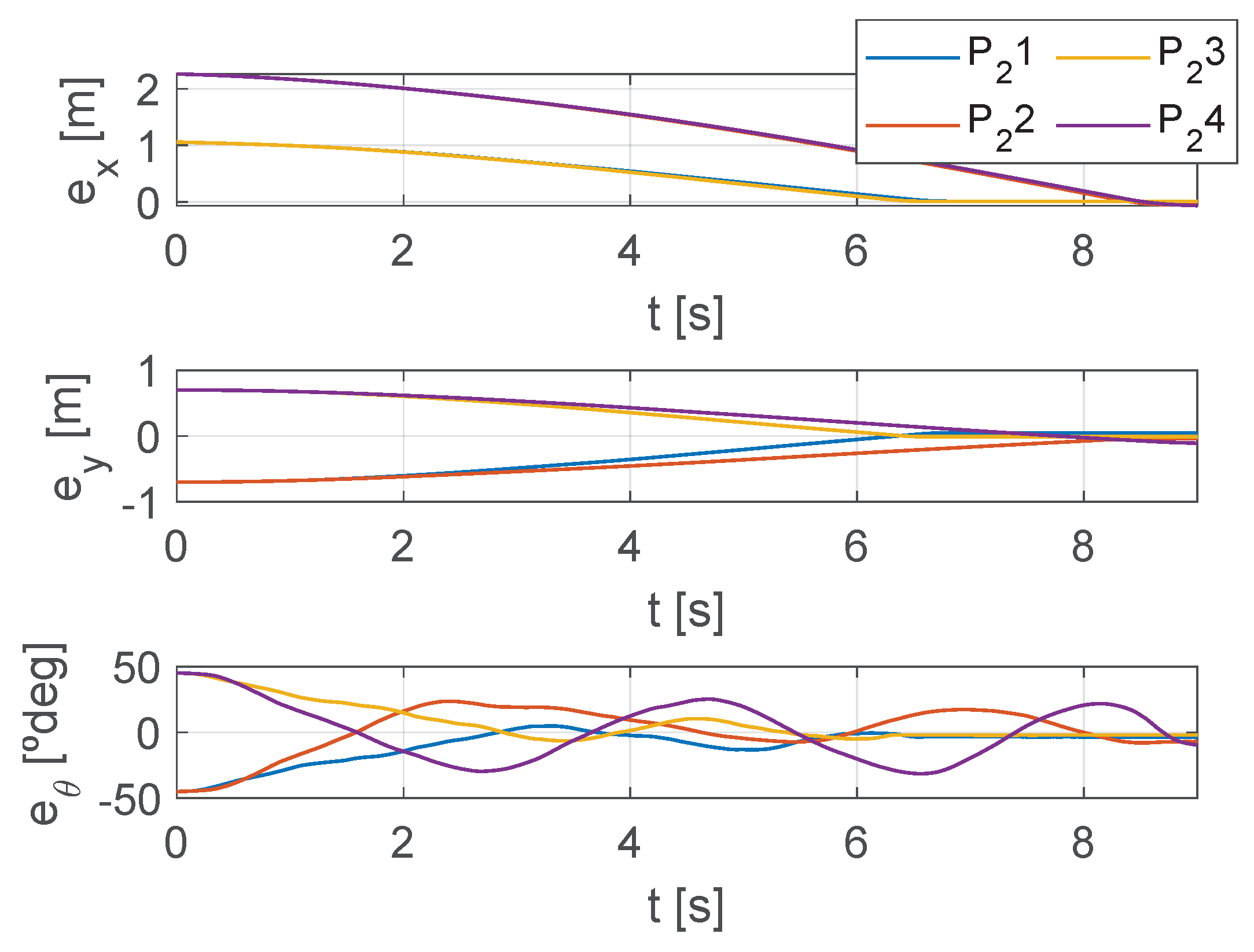
4.3. Results PATH 2

Further exploration of other possible industrial uses of the controlled surface was deemed valuable for the second round of simulations. The application in this case was primarily concerned with package sorting along the line. The envisioned scenario includes an intermediate section of a transport line with side exits, where packages must be directed based on their codes. A graphical example of this is illustrated in Figure 14.

As before, initial and final positions, package characteristics, the surface inputs, and the layout were all predetermined. Instead, the actuation of the modules underneath the transported body at each instant was determined in real time. The Matlab visualization in Figure 15 displays the solutions for carrying out these processes. Both the symbols and the input values, such as the initial speed (0.05 m/s), the surface inclination (8°), and other parameters, are identical to those in the previous subsection. In this case, the only differences are in the target positions (named $P_{2}1$, $P_{2}2$, $P_{2}3$, and $P_{2}4$), which are at the sides of the line at angles of $\pm 45$°, and the layout (footprint 3 m × 2 m). The simulation time was also extended to nine seconds in light of the longer surface that was selected. Although they differ significantly from the PATH 1 case and from one another, the intended configurations are achieved, as seen in Figure 15. This means that the selected controller coefficients $K_p$, $K_i$, and $K_d$ are still in use.

Quantitative reference values are provided for this application as well by reporting the numerical values of the errors at each instant and the settling times. Figure 16 contains the errors data, where trends and oscillations similar to PATH 1 can be observed. Furthermore, for $P_{2}1$, $P_{2}2$ and $P_{2}3$ of Figure 16, the package halting in the desired position is visible. In fact, appreciably earlier than 9 s, as also highlighted by the settling times of

Table 4. Settling time ($St$) with 2% threshold for the two displacements x, y and the orientation $\theta$ in the four outputs cases of PATH2.

	${\mathit{S}\mathit{t}}_{\mathit{x}}$ [s]	${\mathit{S}\mathit{t}}_{\mathit{y}}$ [s]	${\mathit{S}\mathit{t}}_{\mathit{\theta }}$ [s]
$P_{2}1$	$8.748$	$6.748$	$8.381$
$P_{2}2$	$8.744$	$8.543$	$8.715$
$P_{2}3$	$8.197$	$8.457$	$8.631$
$P_{2}4$	$8.984$	$8.957$	$8.983$

, the errors remain constant as the package maintains its target position. This demonstrates that the surface’s effect is continuous throughout the work rather than immediate, with errors not just approaching zero at the chosen simulation time.

Although the issue of sensor delay is explicitly addressed in the context of the threshold-based control, similar considerations are equally relevant for the PID-based strategy. In fact, accurate estimation and management of sensor and processing latency are critical for achieving reliable closed-loop control performance. This aspect has been a key motivation for adopting a digital simulation environment rather than relying solely on the physical prototype. As discussed in Section 2 and Section 4, the current experimental setup is limited by the response time of its onboard sensors, which at present does not yet meet the timing requirements for effective PID implementation. Specifically, the combined delay from sensing, processing, and actuation would need to remain below 0.01 s to align with the performance observed in simulation results, a condition that is still under development in the physical platform. The simulation environment, by contrast, at the moment is not constrained by hardware latency and allows for rapid testing and optimization under idealized timing conditions. Nevertheless, for future physical implementation, the digital model will also require computational efficiency: each simulation cycle must remain fast enough to avoid introducing artificial delays that could compromise control performance.

In summary, one of the layouts selected for these simulations was created in response to the request of the industrial partner, while the other was a possible real-world use case. These examples were reported and utilized to demonstrate how the control mechanism that was designed worked. Theoretically, there are numerous possible simulations that may be customized to fit a variety of industrial activities with different input combinations and layouts. The selected applications in this study were considered suitable for a transport line and offered great complexity, justifying the implementation of a closed-loop PID control system. The outcomes obtained are satisfactory and demonstrate the successful achievement of predefined objectives with accuracy appropriate for their intended purposes. This highlights the feasibility of using the proposed simulation environment to predict spatial configurations within industrial facilities. Furthermore, the possibility of implementing this control system with real-world devices across various applications holds even greater promise.

5. Conclusions

This paper is dedicated to the development and testing of a control system for a novel modular surface for package handling that has been recently investigated. The study begins with an overview of the main features of the concept, its functioning, the digital model, and the objectives. In summary, the concept is an under-actuated rotor-based system, with a camera on top to monitor package motion, and the only controllable variable is the discrete orientation of the rotor axis.

This design inherently imposes specific constraints on the system’s controllability and responsiveness. The under-actuation means that direct control over all degrees of freedom is not possible, limiting the ways the package can be influenced at any given time. Furthermore, the discrete nature of the rotor axis orientation restricts continuous adjustment, confining the system to a finite set of actuation states. These constraints stem directly from the modular and rotor-based architecture chosen to achieve simplicity, modularity, and cost-effectiveness, but they also create challenges in precisely steering the packages, especially under varying conditions.

Due to these characteristics and the working principle, the control strategies proposed in the literature were not directly applicable; therefore, tailored modeling and control methods had to be developed. As a result, two methods were selected: a practical threshold-based control strategy and a dynamic closed-loop control with a PID controller.

For the first method, an existing experimental setup is presented, along with the logic behind its definition. In more detail, the actuation of the surface modules is predefined, and the input condition is governed by the achievement of a limit condition. Practically, two main handling tasks were considered for evaluating the control strategy and system operation with this setup: sorting and orientation. For the sorting task, the threshold condition was simply the package IDs, which determined the type of sorting to be performed. Instead, in the orientation task, the angle variable was continuously monitored throughout the package’s motion. When the angle reached the predefined limit, the actuation was adjusted accordingly. The results in both cases were promising. The sorting and orientation objectives were successfully achieved, with an error of approximately $4.4$% in the second task, where a precise target value had to be reached for the monitored variable.

On the other hand, for the PID control method, the analysis was challenged on two fronts that required some discussion: first, the managing of the severe non-linearities that stem from the under-actuation, over-constrained contact, passive driving and discrete actuation; second, the system modeling had to incorporate novel adjustments to address issues specific to the non-prehensile planar device. As a result, the proposed solution consisted of a feedback system that used the dynamic description of the transported item to retrieve the discrete system’s input variable via minimization. In this context, the developed control was tested using a previously validated software environment, which implements the system’s analytical model. The digital test, having already been certified, provides faster and more cost-effective results without compromising reliability. Specifically, two potential industrial applications of the surface were analyzed. The first was based on a real-world scenario requested by the industrial partner and involved end-of-line sorting with four parallel outputs. The second involved a section of a transport line with lateral outputs. The results include both graphical and numerical demonstrations of the packages reaching the desired positions. For both tests, the initial and final positions, the trajectories of the centers of mass (COM), and the target configurations of the packages on the surface are illustrated. These representations are accompanied by the error trends used in the control law to define the modules and axes to actuate, as well as the settling times that indicate the system’s response speed. Both simulation results highlight the achievement of the predefined tasks. Moreover, the outcomes emphasize the capabilities of the control and the simulation environment. Indeed, any other layout or industrial task could have been quickly chosen and simulated to facilitate physical definition and control feasibility verification. This achievement also marks the culmination of the digital model validations conducted throughout the study [2], as it finally demonstrates the practical applications and potential of the model itself.

Future work will focus on further enhancing the control system and addressing its current limitations. A key step will be the development of a new prototype equipped with faster and more accurate sensors, e.g., a faster camera (increased fps) and a control board with higher computing capacity to avoid the transfer to the external computer. With this sort of upgrade, the setup will enhance real-time monitoring and enable more effective testing of the PID controller under realistic operating conditions. Additionally, a comprehensive robustness analysis will be conducted to evaluate the system’s performance in the presence of variations in critical parameters such as friction coefficients, package dimensions, weights, etc. Lastly, another aspect that could benefit from further refinement is the tuning of the PID controller gains ($K_p$, $K_i$, $K_d$), which can be further refined by exploring and testing different parameter selection techniques available in the literature. These efforts will contribute to improving control accuracy and system reliability in practical applications.

References

- Uriarte, C.; Asphandiar, A.; Thamer, H.; Thamer, H.; Benggolo, A.Y.; Freitag, M. Control strategies for small-scaled conveyor modules enabling highly flexible material flow systems. Procedia CIRP 2018, 79, 433–438. [Google Scholar] [CrossRef]
- Bianchi, E.; Fantoni, G.; Dueso, F.J.B.; Yagüe-Fabra, J.A. A novel underactuated smart surface for parts feeding and sorting. Int. J. Adv. Manuf. Technol. 2024, 135, 1221–1239. [Google Scholar] [CrossRef]
- Matignon, L.; Laurent, G.J.; Le Fort-Piat, N. Design of semi-decentralized control laws for distributed-air-jet micromanipulators by reinforcement learning. In Proceedings of the 2009 IEEE/RSJ International Conference on Intelligent Robots and Systems, St. Louis, MO, USA, 10–15 October 2009; pp. 3277–3283. [Google Scholar] [CrossRef]
- El Baz, D.; Boyer, V.; Bourgeois, J.; Dedu, E.; Boutoustous, K. Distributed part differentiation in a smart surface. Mechatronics 2012, 22, 522–530. [Google Scholar] [CrossRef]
- Boutoustous, K.; Laurent, G.J.; Dedu, E.; Matignon, L.; Bourgeois, J.; Le-Fort-Piat, N. Distributed control architecture for smart surfaces. In Proceedings of the 2010 IEEE/RSJ International Conference on Intelligent Robots and Systems, Taipei, Taiwan, 18–22 October 2010. [Google Scholar] [CrossRef]
- Bohringer, K.F.; Donald, B.R.; MacDonald, N.C. Programmable force fields for distributed manipulation, with applications to MEMS actuator arrays and vibratory parts feeders. Int. J. Robot. Res. 1999, 18, 168–200. [Google Scholar] [CrossRef]
- Mobes, S.; Laurent, G.J.; Clevy, C.; Fort-Piat, N.L.; Piranda, B.; Bourgeois, J. Toward a 2D Modular and Self-Reconfigurable Robot for Conveying Microparts. In Proceedings of the 2012 Second Workshop on Design, Control and Software Implementation for Distributed MEMS, Besancon, France, 2–3 April 2012; pp. 7–13. [Google Scholar] [CrossRef]
- Skima, H.; Varnier, C.; Dedu, E.; Medjaher, K.; Bourgeois, J. Post-prognostics decision making in distributed MEMS-based systems. J. Intell. Manuf. 2019, 30, 1125–1136. [Google Scholar] [CrossRef]
- Bedillion, M.; Messner, W. Control for actuator arrays. Int. J. Robot. Res. 2009, 28, 868–882. [Google Scholar] [CrossRef]
- Murphey, T.D.; Burdick, J.W. Feedback control methods for distributed manipulation systems that involve mechanical contacts. Int. J. Robot. Res. 2004, 23, 763–781. [Google Scholar] [CrossRef]
- Keek, J.S.; Loh, S.L.; Chong, S.H. Design and Control System Setup of an E-Pattern OmniwheeledCellular Conveyor. Machines 2021, 9, 43. [Google Scholar] [CrossRef]
- Bianchi, E.; Brosed Dueso, F.J.; Yagüe-Fabra, J.A. In-Plane Material Handling: A Systematic Review. Appl. Sci. 2024, 14, 7302. [Google Scholar] [CrossRef]
- Krühn, T.; Falkenberg, S.; Overmeyer, L. Decentralized control for small-scaled conveyor modules with cellular automata. In Proceedings of the 2010 IEEE International Conference on Automation and Logistics, Hong Kong, China, 16–20 August 2010; pp. 237–242. [Google Scholar] [CrossRef]
- Bianchi, E.; Jorg, O.J.; Fantoni, G.; Brosed Dueso, F.J.; Yagüe-Fabra, J.A. Study and Simulation of an Under-Actuated Smart Surface for Material Flow Handling. Appl. Sci. 2023, 13, 1937. [Google Scholar] [CrossRef]
- Luntz, J.E.; Messner, W.; Choset, H. Distributed Manipulation Using Discrete Actuator Arrays. Int. J. Robot. Res. 2001, 20, 553–583. [Google Scholar] [CrossRef]
- Lynch, K.M.; Murphey, T.D. Control of nonprehensile manipulation. In Control Problems in Robotics; Springer: Berlin/Heidelberg, Germany, 2003; pp. 39–57. [Google Scholar]
- Elahidoost, A.; Keshmiri, M. Final position and trajectory control of an object on a distributed manipulation system. In Proceedings of the 2009 6th International Symposium on Mechatronics and its Applications, Sharjah, United Arab Emirates, 23–26 March 2009; pp. 1–6. [Google Scholar] [CrossRef]
- Bedillion, M.; Messner, W. Trajectory Tracking Control for Actuator Arrays. IEEE Trans. Control Syst. Technol. 2013, 21, 2341–2349. [Google Scholar] [CrossRef]
- Bianchi, E.; Jorg, O.J.; Fantoni, G.; Brosed Dueso, F.J.; Yagüe-Fabra, J.A. Design and development of a not actively driven modular device for parts feeding and sorting. Mech. Based Des. Struct. Mach. 2024, 52, 10124–10147. [Google Scholar] [CrossRef]
- Spindler, M.; Aicher, T.; Schütz, D.; Vogel-Heuser, B.; Günthner, W.A. Modularized control algorithm for automated material handling systems. In Proceedings of the 2016 IEEE 19th International Conference on Intelligent Transportation Systems (ITSC), Rio de Janeiro, Brazil, 1–4 November 2016; pp. 2644–2650. [Google Scholar] [CrossRef]
- Olson, E. AprilTag: A robust and flexible visual fiducial system. In Proceedings of the 2011 IEEE International Conference on Robotics and Automation, Shanghai, China, 9–13 May 2011; pp. 3400–3407. [Google Scholar] [CrossRef]
- Bianchi, E.; Yagüe Fabra, J.A.; Brosed Dueso, F.J. Design and Development of a Novel Under-Actuated Smart Surface for Material Flow Handling. Ph.D. Thesis, Universidad de Zaragoza, Zaragoza, Spain, 7 November 2024. [Google Scholar]
- Visioli, A. Practical PID Control; Springer Science & Business Media: Berlin/Heidelberg, Germany, 2006. [Google Scholar]
- MATLAB Documentation Set, Version 2022b; The MathWorks: Natick, MA, USA, 2022.
- Euzébio, T.A.M.; Silva, M.T.D.; Yamashita, A.S. Decentralized PID Controller Tuning Based on Nonlinear Optimization to Minimize the Disturbance Effects in Coupled Loops. IEEE Access 2021, 9, 156857–156867. [Google Scholar] [CrossRef]
- Torga, D.S.; da Silva, M.T.; Reis, L.A.; Euzébio, T.A. Simultaneous tuning of cascade controllers based on nonlinear optimization. Trans. Inst. Meas. Control 2022, 44, 3118–3131. [Google Scholar] [CrossRef]
- Wai, R.J.; Lee, J.D.; Chuang, K.L. Real-Time PID Control Strategy for Maglev Transportation System via Particle Swarm Optimization. IEEE Trans. Ind. Electron. 2011, 58, 629–646. [Google Scholar] [CrossRef]