Spike-Driven Channel-Temporal Attention Network with Multi-Scale Convolution for Energy-Efficient Bearing Fault Detection

Abstract

Real-time bearing fault diagnosis necessitates highly accurate, computationally efficient, and energy-conserving models suitable for deployment on resource-constrained edge devices. To address these demanding requirements, we propose the Spike Convolutional Attention Network (SpikeCAN), a novel spike-driven neural architecture tailored explicitly for real-time industrial diagnostics. SpikeCAN utilizes the inherent sparsity and event-driven processing capabilities of spiking neural networks (SNNs), significantly minimizing both computational load and power consumption. The SpikeCAN integrates a multi-dilated receptive field (MDRF) block and a convolution-based spike attention module. The MDRF module effectively captures extensive temporal dependencies from signals across various scales. Simultaneously, the spike-based attention mechanism dynamically extracts spatial-temporal patterns, substantially improving diagnostic accuracy and reliability. We validate SpikeCAN on two public bearing fault datasets: the Case Western Reserve University (CWRU) and the Society for Machinery Failure Prevention Technology (MFPT). The proposed model achieves 99.86% accuracy on the four-class CWRU dataset through five-fold cross-validation and 99.88% accuracy with a conventional 70:30 train–test random split. For the more challenging ten-class classification task on the same dataset, it achieves 97.80% accuracy under five-fold cross-validation. Furthermore, SpikeCAN attains a state-of-the-art accuracy of 96.31% on the fifteen-class MFPT dataset, surpassing existing benchmarks. These findings underscore a significant advancement in fault diagnosis technology, demonstrating the considerable practical potential of spike-driven neural networks in real-time, energy-efficient industrial diagnostic applications.

1. Introduction

Bearings are critical mechanical components that significantly influence the reliability, performance, and efficiency of various industrial systems, such as automotive engines, aerospace equipment, and wind turbines [1]. These bearings typically operate in environments characterized by high rotational speeds, heavy loads, elevated temperatures, and constant vibration, collectively defined as demanding operational conditions [2]. Such conditions significantly accelerate the wear and deterioration of bearings, increasing their susceptibility to faults. Numerous studies have consistently indicated that bearing faults account for over half of all mechanical system failures, leading to substantial economic losses due to unplanned downtime, costly repairs, and decreased productivity [3,4]. Consequently, the development of accurate and efficient real-time fault detection and diagnosis methodologies is crucial for enhancing system reliability and operational safety.

Traditionally, bearing fault diagnosis approaches typically involve manual extraction of discriminative features from vibration signals and classic machine learning algorithms [5]. While these techniques can be effective, they heavily rely on expert domain knowledge and are highly sensitive to noise and varying operating conditions. To overcome these limitations, researchers have increasingly adopted deep-learning-based methods, benefiting from their automated feature extraction capabilities and robust performance in noisy environments. In particular, convolutional neural networks (CNNs), renowned for their effectiveness in image processing tasks, have demonstrated significant success in bearing fault diagnosis applications [6,7]. However, bearing vibration signals inherently possess temporal characteristics that CNN architectures alone may inadequately capture. This shortcoming has motivated further exploration into sequence-based models, such as recurrent neural networks (RNNs) [8,9] and transformer architectures [10,11], both of which have shown improved capability in modeling temporal dependencies.

Despite the demonstrated performance improvements, deploying conventional deep learning architectures in practical, real-time industrial scenarios remains challenging. These deep networks usually feature a large number of parameters and complex computations, resulting in significant memory usage and computational costs [12,13,14,15]. Such characteristics limit their suitability for real-time monitoring, especially in resource-constrained edge computing environments where power consumption and inference speed are critical considerations. Edge computing devices facilitate early fault detection and immediate response actions, significantly reducing the risk of minor faults escalating into severe breakdowns [16]. Additionally, processing data locally on edge devices reduces the communication burden on centralized systems, supports autonomous operation in remote or inaccessible installations, and enhances overall system efficiency through reduced energy consumption. These advantages become increasingly important for real-time monitoring in large-scale or remotely situated industrial systems.

In response to these challenges, spiking neural networks (SNNs) [17] have emerged as a compelling alternative. SNNs process information using discrete binary spike signals and operate based on an event-driven computing paradigm, substantially reducing energy consumption compared to traditional neural networks. Specifically, the SNN architecture replaces computationally intensive multiply-and-accumulate (MAC) operations with simpler accumulate (AC) operations, exploiting their inherent sparsity and asynchronous processing nature [18]. Their asynchronous, event-driven nature keeps the network largely inactive until meaningful input spikes arrive, thereby further lowering power requirements. This advantage is especially suitable for real-time industrial monitoring scenarios, where memory and computational resources are limited but inference speed is critical. Nevertheless, spike-driven SNNs commonly exhibit lower performance accuracy compared to conventional deep neural networks, primarily due to the sparsity and limited information representation of spike signals [19].

To mitigate this performance degradation, hybrid neural network architectures combining SNNs and artificial neural networks (ANNs) have been proposed [20]. These approaches typically integrate SNNs with ANN-based modules to enhance accuracy. However, they inevitably reintroduce MAC operations, undermining the computational and energy-efficiency benefits of purely spike-driven systems. As a result, research has increasingly shifted toward improving performance within fully spike-driven architectures that preserve the energy efficiency of SNNs.

A key challenge in this pursuit is converting continuous-valued input signals into spike trains. Among the various encoding techniques explored—such as rate coding [21] and temporal coding [22]—direct encoding has shown notable advantages. By mapping continuous values directly into spike magnitudes at each timestep, direct encoding effectively retains informative content with fewer timesteps, thereby reducing latency and memory requirements [23,24]. In parallel, the inherent non-differentiability of spike signals has been addressed using surrogate gradient learning methods, which approximate gradients and enable efficient backpropagation training in spike-based networks [25].

Building upon these foundational advancements, attention-based SNN models—such as SEW-ResNet—have emerged, demonstrating that spike-driven architectures can achieve performance comparable to ANN counterparts while maintaining significantly lower energy consumption [18,26,27,28]. These innovations have made it possible to build SNN models that perform well while still using much less energy and computing power. Despite recent advances in SNNs, existing approaches for bearing fault diagnosis have yet to simultaneously achieve ANN-level accuracy and genuine event-driven efficiency. Furthermore, previous SNN methods have not effectively incorporated attention mechanisms to dynamically weight spatial-temporal features and adequately extend receptive fields, which is crucial for processing long-sequence vibration signals commonly encountered in bearing fault diagnosis.

Motivated by these developments, we propose the spike convolutional attention network (SpikeCAN), a fully spike-driven architecture explicitly tailored for energy-efficient, real-time bearing fault diagnosis. SpikeCAN incorporates two novel modules: the spike attention module and the multi-dilated receptive field (MDRF) convolutional module. The spike attention module dynamically emphasizes critical spatial-temporal features, whereas the MDRF module efficiently captures extensive temporal dependencies through dilated convolutions and multi-scale kernels. Additionally, SpikeCAN employs carefully designed residual connections to alleviate spike-vanishing issues, thereby ensuring robust training and enhanced accuracy.

We comprehensively evaluate the proposed SpikeCAN model using two prominent benchmark datasets in the bearing fault diagnosis domain: the Case Western Reserve University (CWRU) dataset [29] and the Society for Machinery Failure Prevention Technology (MFPT) dataset [30]. Our results demonstrate outstanding accuracy, with SpikeCAN achieving 99.86% accuracy on the four-class classification task of the CWRU dataset using five-fold cross-validation and 99.88% accuracy under a conventional 70:30 train–test split averaged over five random seeds. Additionally, SpikeCAN achieves a notable 96.31% accuracy on the challenging fifteen-class MFPT dataset, surpassing existing spike-driven approaches and establishing a new state-of-the-art benchmark. Overall, our findings underscore the potential of SpikeCAN to significantly advance energy-efficient, real-time bearing fault diagnosis, highlighting its practical applicability in industrial settings.

The remainder of this paper is structured as follows. Section 2 provides a review of related work and discusses the motivation behind the proposed approach. Section 3 introduces the SpikeCAN model, detailing its architecture and key mechanisms. In Section 4, we describe the experimental setup and datasets used in this study. Section 5 presents the evaluation methods along with comprehensive results and analyses. Section 6 outlines the methodology employed to calculate energy consumption. Section 7 reports on detailed ablation studies to validate the effectiveness of individual components and the model’s robustness to variations in training sample size. Finally, Section 8 provides conclusions and discussions along with potential future research directions.

2. Related Work

2.1. Spiking Nerual Network

SNNs are often referred to as third-generation neural networks because they more closely mimic the behavior of biological neurons than traditional ANNs. Unlike ANNs, which process continuous-valued signals, SNNs transmit information over time using discrete binary spike events [17]. To enable this form of computation, SNNs rely on specialized spiking neurons that convert input signals into binary spikes. Among the commonly used spiking neuron models, the leaky integrate-and-fire (LIF) and the more recent parametric leaky integrate-and-fire (PLIF) neurons are widely adopted [31]. The PLIF model incorporated a learnable membrane time constant, allowing the neuron to adapt its temporal dynamics during training. Its behavior is mathematically described as follows:

$$V\left[t\right]=V[t-1]+{\displaystyle \frac{1}{\tau }}\left(X\left[t\right]-\left(V[t-1]-V_{\mathrm{reset}}\right)\right)$$

(1)

where $V\left[t\right]$ represents the membrane potential at time step t, $X\left[t\right]$ denotes the input synaptic current, $\tau$ is a learnable time constant, and $V_{\mathrm{reset}}$ is the resting membrane potential. When $V\left[t\right]$ exceeds a predefined threshold, the neuron emits a spike and resets its membrane potential.

SNNs can be trained using two primary strategies: direct training [23] and ANN-to-SNN conversion [32]. In the direct training approach [23], the SNN is optimized end-to-end using backpropagation through time (BPTT). However, because the spiking function is inherently non-differentiable, surrogate gradient techniques [25] are employed to approximate gradients and allow effective training via gradient descent. Alternatively, the ANN-to-SNN conversion method [32] first trains a conventional ANN with continuous activation functions, which are then replaced with spiking neuron models such as LIF or PLIF. The trained weights are mapped directly to the corresponding SNN architecture. Although this approach benefits from the mature training techniques of ANNs, it often struggles to preserve fine-grained temporal dynamics and typically requires a large number of time steps during inference in increased latency.

2.2. SNNs for Industrial Fault Diagnosis

Bearing fault diagnosis tasks inherently require continuous, real-time monitoring to detect faults and initiate immediate corrective actions promptly. Such monitoring typically occurs directly on edge devices, which must operate effectively under significant constraints in terms of computational resources, energy consumption, and available bandwidth. Processing data locally at the edge not only minimizes delays in fault detection but also reduces communication overhead with centralized servers, enabling autonomous operation in remote or inaccessible industrial settings. Under these demanding conditions, SNNs, characterized by their event-driven computation and significantly low energy consumption due to sparse spike-based processing, emerge as highly promising solutions for bearing fault diagnosis. The spike-driven nature of SNNs substantially reduces their computational load and energy requirements, making them exceptionally suitable for real-time monitoring on resource-constrained edge devices. Additionally, SNNs possess the intrinsic capability to effectively handle diverse input signals, dynamically modulating their internal membrane potentials in response, which can enhance their learning capabilities and diagnostic performance [33]. Bearing fault signals inherently contain a wide spectrum of distinct patterns corresponding to various operational and fault states, aligning effectively with this advantageous characteristic of SNNs.

To date, only a few studies [34,35] have explicitly explored the application of SNNs for bearing fault diagnosis. Both start from an efficient constraint of how to turn continuous vibration magnitudes into spikes. The earlier study [34] employed Gaussian Receptive Field (GRF) population coding, where each measurement is translated into spike timings using multiple Gaussian functions. The resulting spikes are classified using a simple network composed of Pulse-Stream Rate Model (PSRM) neurons using a shallow, fully connected multi-layer network. The PSRM structure was selected mainly due to its simplicity and ease of use with limited training data. The follow-up study [35] further improved the GRF encoding method and added another hidden layer.

Both models heavily rely on handcrafted feature extraction techniques, local mean decomposition (LMD), which decomposes vibration signals into amplitude- and frequency-modulated components, such as skewness, kurtosis, and crest factor. Although LMD effectively extracts bearing-related modes, these multi-stage pipelines introduce considerable computational complexity, require extensive domain expertise, and incur increased energy consumption due to non-spiking operation. The reliance on non-spike-driven preprocessing diminishes the fundamental energy efficiency advantages of SNNs, limiting the feasibility of end-to-end spike-driven processing for deployment in real-time, energy-constrained edge computing environments. Moreover, because these approaches rely on shallow networks with limited capacity, they struggle to capture complex temporal patterns present in bearing faults.

In contrast, our proposed SpikeCAN model directly processes raw vibration signals in a fully spike-driven manner, obviating the need for separate feature extraction stages. SpikeCAN is also built upon a deep SNN framework integrated with spike-compatible attention mechanisms, enabling autonomous learning of salient temporal and spatial features. Attention mechanisms have become essential for enhancing interpretability and performance in deep neural networks. The convolutional block attention module (CBAM) [36] efficiently derives channel and spatial attention maps through sequential pooling and convolution operations, proving effective primarily within convolutional architectures tailored for spatial data. Nevertheless, the spatially oriented design of CBAM limits its direct applicability to time-series datasets. Alternatively, Transformer-based self-attention mechanisms [10], employing scaled dot-product computations among query, key, and value vectors, offer powerful global context modeling capabilities, yet their heavy computational complexity makes them challenging to deploy in resource-constrained environments.

To overcome these limitations, we propose novel spike-compatible attention modules: spike channel attention (SCA) and spike temporal attention (STA). These modules leverage the computational efficiency of CBAM but are explicitly adapted for spike-driven neural networks processing time-series data. Specifically, we replace the spatial attention component of CBAM with STA, enabling the effective capture of temporal dependencies. Furthermore, to maintain spike-based processing and minimize information loss, our design employs spike-based addition rather than continuous-valued computations or multiplicative operations. This carefully constructed mechanism preserves spike-timing precision, essential for accurate temporal feature extraction, while significantly reducing computational overhead, thus enabling energy-efficient deployment on neuromorphic hardware.

3. Method

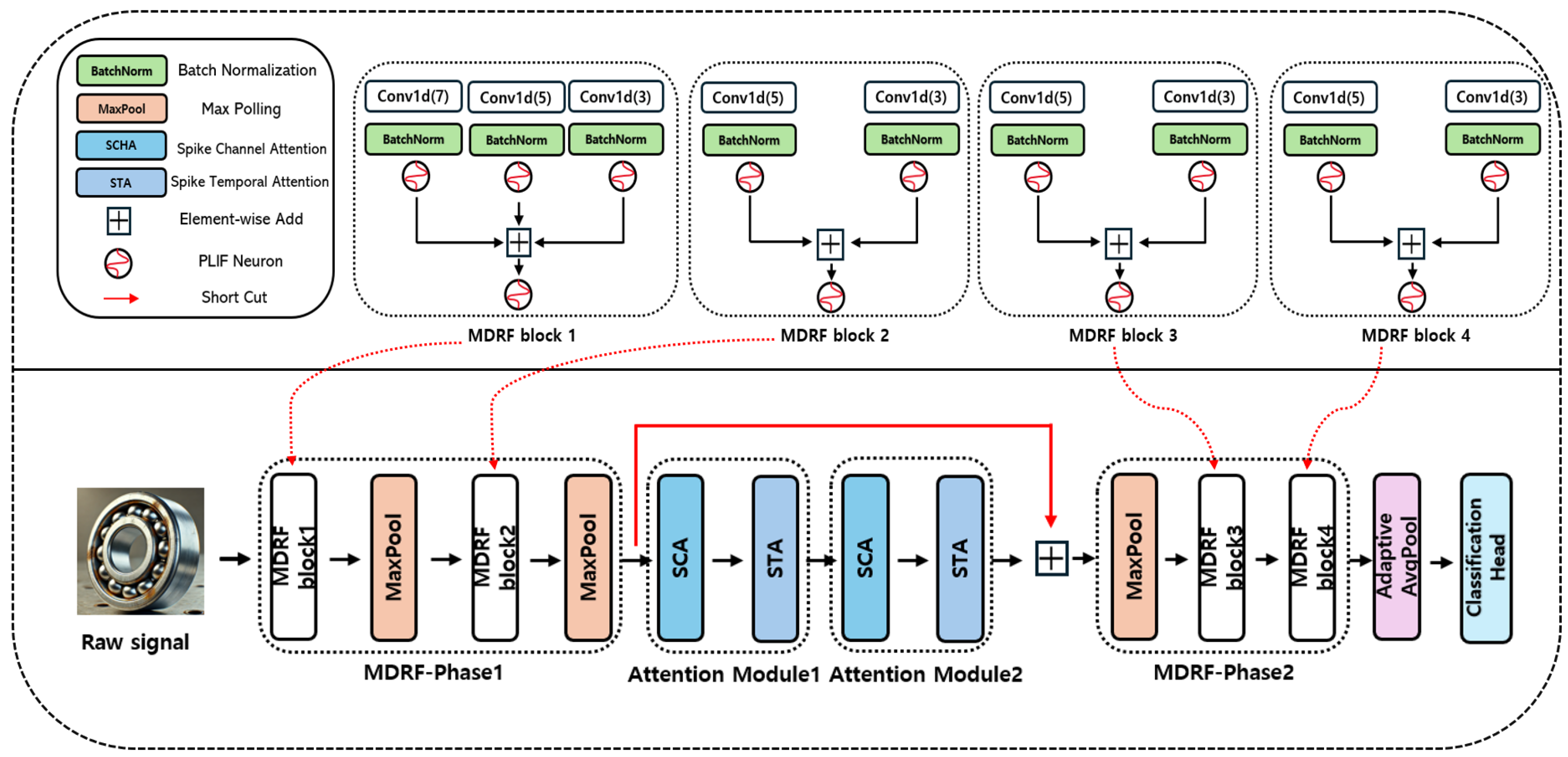
In this study, we propose SpikeCAN, a spike-driven SNN architecture for bearing fault diagnosis. SpikeCAN supports end-to-end learning from raw input signals without requiring any handcrafted feature extraction or signal preprocessing. Designed entirely within the spike domain, the model is optimized for low energy consumption and is well-suited for deployment on edge devices with constrained computational resources.

SpikeCAN is composed of three main components: the MDRF block, SCA block, and STA block. The overall architecture of the proposed model is illustrated in Figure 1. The hyperparameters employed in the model were systematically determined through a grid search over several candidate values based on commonly adopted configurations from established literature [36]. The model processes input data in three sequential stages. First, the input signal is passed through MDRF-Phase 1, which extracts global temporal features using multi-scale convolutional processing. Next, the output is refined using two consecutive attention modules, each composed of an SCA block followed by an STA block, enabling the model to adaptively focus on relevant features. Finally, the resulting spike-based features are processed by MDRF-Phase 2 to extract localized patterns, followed by adaptive average pooling and a classification head to produce the final prediction.

3.1. MDRF-Phase 1

MDRF-Phase 1 serves as the initial feature extraction stage. It takes the raw input spike train and processes it through two sequential MDRF blocks, each followed by a MaxPooling operation. This stage is designed to capture global and long-range temporal dependencies in the input signal by leveraging wide receptive fields enabled by dilated convolutions.

Formally, given input $x_0$, the operations in this phase can be described as:

$$\begin{array}{cc}\hfill X_1& ={\mathrm{MDRF}}_1\left(x_0\right),\hfill \end{array}$$

(2)

$$\begin{array}{cc}\hfill X_2& =\mathrm{MaxPool}(X_1,kernel=2,stride=2),\hfill \end{array}$$

(3)

$$\begin{array}{cc}\hfill X_3& ={\mathrm{MDRF}}_2\left(X_2\right),\hfill \end{array}$$

(4)

$$\begin{array}{cc}\hfill X_4& =\mathrm{MaxPool}(X_3,kernel=2,stride=2).\hfill \end{array}$$

(5)

Each MDRF block applies multiple 1D convolutions in parallel using different kernel sizes and dilation rates to extract multi-scale temporal features. The resulting spike maps are fused using spike-domain operations and passed through a PLIF neuron to generate spike outputs.

3.2. Attention Module 1 and 2

After the initial feature extraction, the feature $X_4$ is further refined through two attention modules, each composed of an SCA block followed by an STA block. These modules allow the network to adaptively highlight discriminative features along both the channel and temporal dimensions. The flow of computation through the attention modules is as follows:

$$\begin{array}{cc}\hfill X_5& =\mathrm{SCA}\left(X_4\right),\hfill \end{array}$$

(6)

$$\begin{array}{cc}\hfill X_6& =\mathrm{STA}\left(X_5\right),\hfill \end{array}$$

(7)

$$\begin{array}{cc}\hfill X_7& =\mathrm{SCA}\left(X_6\right),\hfill \end{array}$$

(8)

$$\begin{array}{cc}\hfill X_8& =\mathrm{STA}\left(X_7\right),\hfill \end{array}$$

(9)

$$\begin{array}{cc}\hfill \mathrm{ATT}& =X_4+X_8,\hfill \end{array}$$

(10)

where the final attention output of the attention stage, denoted as $\mathrm{ATT}$, is computed by applying spike-element-wise addition between the output of the second STA block ($X_8$) and the input of the first attention module ($X_4$). This residual connection helps preserve the original feature information while integrating refined attention-enhanced features.

3.3. MDRF-Phase 2

MDRF-Phase 2 aims to capture more fine-grained local features using smaller kernels and reduced dilation. This phase begins with a MaxPooling operation to reduce the temporal resolution, followed by two additional MDRF blocks (MDRF-block 3 and MDRF-block 4), which further refine the feature representation learned in the earlier stages. The processing flow is defined as:

$$\begin{array}{cc}\hfill X_9& =\mathrm{MaxPool}(\mathrm{ATT},kernel=2,stride=2),\hfill \end{array}$$

(11)

$$\begin{array}{cc}\hfill X_{10}& ={\mathrm{MDRF}}_3\left(X_9\right),\hfill \end{array}$$

(12)

$$\begin{array}{cc}\hfill X_{11}& ={\mathrm{MDRF}}_4\left(X_{10}\right).\hfill \end{array}$$

(13)

This stage completes the hierarchical feature extraction process, preparing the spike-based feature map for the final classification stage.

3.4. MDRF Block

Bearing fault diagnosis typically involves time-series signals that require capturing both short- and long-range temporal dependencies. Although Transformer-based models have proven effective for this purpose, their high computational cost often limits their deployment in real-time or edge computing scenarios. To address these limitations, we propose a convolution-based MDRF block that enables efficient temporal modeling while maintaining low computational complexity.

The MDRF block employs parallel 1D convolutions with different kernel sizes and dilation rates to construct a multi-scale receptive field. This design captures temporal features at various scales, reducing information loss that might occur in single-scale architectures. Structurally, four MDRF blocks—MDRF-block 1 through MDRF-block 4—are incorporated into SpikeCAN. Specifically, MDRF-block 1 uses three parallel 1D convolution (Conv1d) layers with kernel sizes $k\in \{3,5,7\}$ and dilation factors $D\in \{1,2,4\}$ applied to the batch-normalized input. The outputs are summed element-wise and passed through a PLIF neuron to generate spike activations:

$$\begin{array}{cc}\hfill {\mathrm{RP}}_7& =\mathrm{Conv}1\mathrm{d}\left(\mathrm{BatchNorm}\left(x_0\right),k=7,D=4\right),\hfill \end{array}$$

(14)

$$\begin{array}{cc}\hfill {\mathrm{RP}}_5& =\mathrm{Conv}1\mathrm{d}\left(\mathrm{BatchNorm}\left(x_0\right),k=5,D=2\right),\hfill \end{array}$$

(15)

$$\begin{array}{cc}\hfill {\mathrm{RP}}_3& =\mathrm{Conv}1\mathrm{d}\left(\mathrm{BatchNorm}\left(x_0\right),k=3,D=1\right),\hfill \end{array}$$

(16)

$$\begin{array}{cc}\hfill {\mathrm{RP}}_{\mathrm{add}}& ={\mathrm{RP}}_7+{\mathrm{RP}}_5+{\mathrm{RP}}_3,\hfill \end{array}$$

(17)

$$\begin{array}{cc}\hfill {\mathrm{MDRF}}_1& =\mathrm{PLIF}\left({\mathrm{RP}}_{\mathrm{add}}\right).\hfill \end{array}$$

(18)

In contrast, MDRF-blocks 2, 3, and 4 are designed to be lighter in computational cost. Each of these blocks utilizes two convolution branches with kernel sizes of 3 and 5 and corresponding dilation factors of 1 and 2. For each block, the outputs are batch-normalized, fused via element-wise addition, and passed through a PLIF neuron to produce spike-based outputs. This structure allows efficient local feature extraction while preserving compatibility with event-driven SNN processing.

Additionally, each of these blocks is followed by a MaxPooling operation to reduce the temporal resolution, helping to lower the computational load and mitigate feature redundancy. Formally, for each input $X_j\in \{X_2,X_9,X_{10}\}$, the computation proceeds as:

$$\begin{array}{cc}\hfill {\mathrm{RP}}_5& =\mathrm{Conv}1\mathrm{d}\left(\mathrm{BatchNorm}\left(X_j\right),k=5,D=2\right),j\in \{2,9,10\},\hfill \end{array}$$

(19)

$$\begin{array}{cc}\hfill {\mathrm{RP}}_3& =\mathrm{Conv}1\mathrm{d}\left(\mathrm{BatchNorm}\left(X_j\right),k=3,D=1\right),j\in \{2,9,10\}.\hfill \end{array}$$

(20)

$$\begin{array}{cc}\hfill {\mathrm{RP}}_{\mathrm{add}}& ={\mathrm{RP}}_5+{\mathrm{RP}}_3,\hfill \end{array}$$

(21)

$$\begin{array}{cc}\hfill {\mathrm{MDRF}}_i& =\mathrm{PLIF}\left({\mathrm{RP}}_{\mathrm{add}}\right),i\in \{2,3,4\}.\hfill \end{array}$$

(22)

In this manner, MDRF-block 1 extracts richer temporal representations using three convolution branches, while MDRF-blocks 2 through 4 offer computationally efficient alternatives optimized for real-time applications.

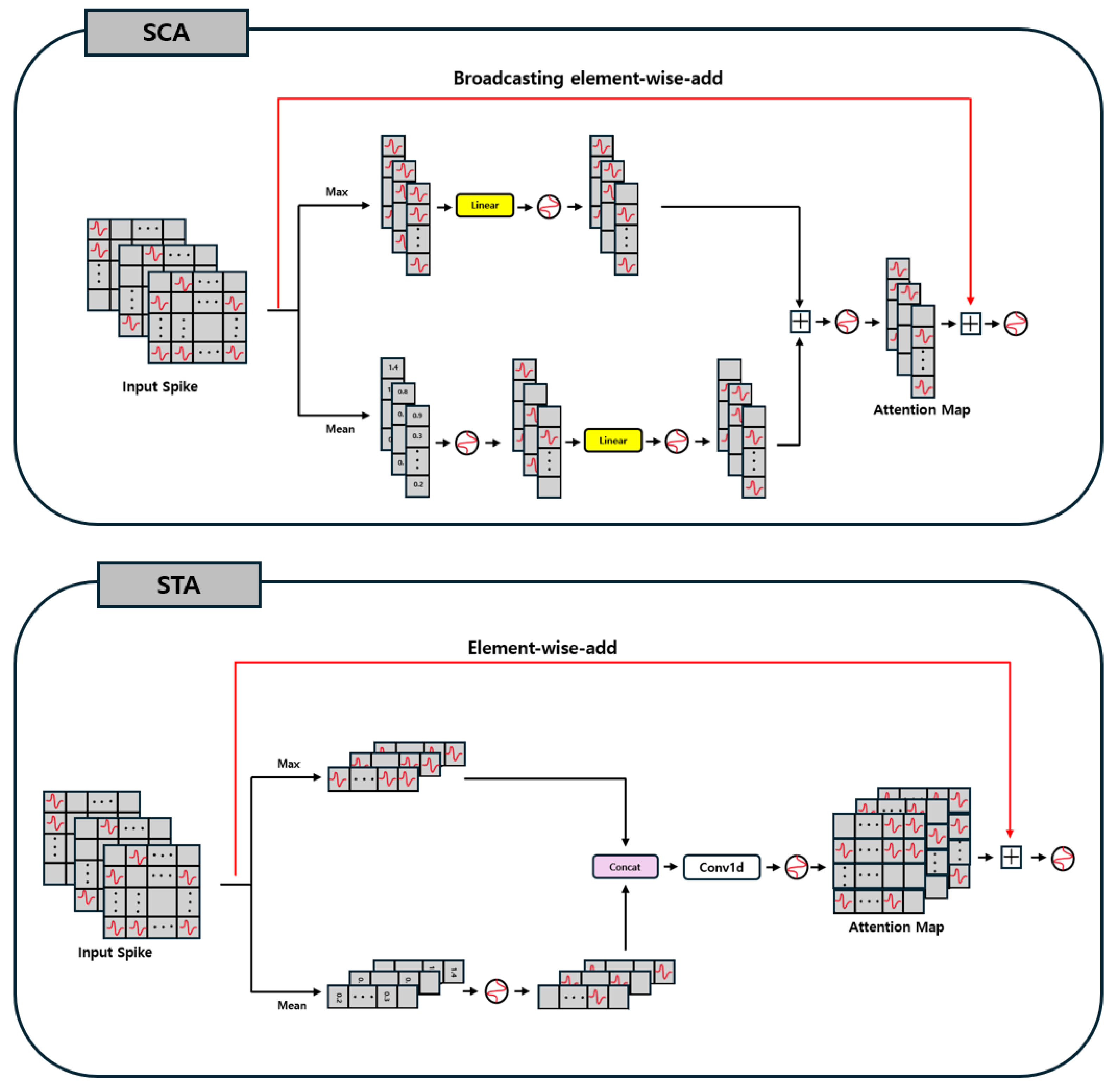
3.5. Spike Convolutional Attention

We introduce two convolution-based attention blocks, SCA and STA, specifically designed for spike-driven SNNs. These methods effectively adapt conventional ANN-based convolutional attention mechanisms for spike-based processing, enabling SNNs to achieve maximal performance improvements while fully maintaining spike-driven computations. The overall architecture of SCA and STA is shown in Figure 2.

First, both SCA and STA perform their internal operations using spike signals composed of $\{0,1\}$. As a result, most of MAC operations in conventional convolutional attention can be replaced with AC operations, thereby reducing computational cost. Moreover, due to the nature of spike signals, which never produce negative values during computation, non-linear operations such as the sigmoid and exponential functions become unnecessary, further decreasing the overall calculation overhead.

Additionally, we introduce a spike-compatible attention integration method termed spike addition, which leverages the binary nature of spike signals. Because spike signals consist of $\{0,1\}$, the attention maps in SCA and STA are also represented by $\{0,1\}$. When added to the original spike features, the resulting values become $\{0,1,2\}$. Here, 0 denotes unimportant information, 1 indicates that a spike occurred in either the attention map or the original feature alone, and 2 indicates that spikes occurred in both simultaneously. By employing this spike addition method, the attention map can be applied to the original features effectively while minimizing any loss of spike information.

3.5.1. SCA Block

The SCA block is a convolution-based attention mechanism designed to emphasize channel-specific information in the input. Its operation proceeds as follows: first, the mean and maximum values are computed along the temporal axis. The mean value captures the overall distribution of the data, while the maximum value highlights salient regions. Given the spiking nature of the model, the mean value is processed by a PLIF neuron to be converted back into a spike signal.

Then, each value is passed through its own linear layer for training and is subsequently transformed into a spike signal via another PLIF neuron. These two spike signals are combined using a spike-element-wise addition. The resulting feature map is again fed into a PLIF neuron to generate the final spike channel attention map, which is subsequently added to the original input through a spike-element-wise addition to perform the channel attention mechanism.

The computation steps of SCA are given by:

$$\begin{array}{cc}\hfill x_{max}& =max\left(X_4,\mathrm{axis}=\mathrm{temporal}\right),\hfill \end{array}$$

(23)

$$\begin{array}{cc}\hfill x_{\mathrm{mean}}& =\mathrm{PLIF}\left(\mathrm{mean}(X_4,\mathrm{axis}=\mathrm{temporal})\right),\hfill \end{array}$$

(24)

$$\begin{array}{cc}\hfill x_{max}& =\mathrm{Linear}\left(x_{max}\right),x_{\mathrm{mean}}=\mathrm{Linear}\left(x_{\mathrm{mean}}\right),\hfill \end{array}$$

(25)

$$\begin{array}{cc}\hfill \mathrm{Att}\_\mathrm{map}& =\mathrm{PLIF}(x_{max}+x_{\mathrm{mean}}),\hfill \end{array}$$

(26)

$$\begin{array}{cc}\hfill \mathrm{Ch}\_\mathrm{att}& =x+\mathrm{Att}\_\mathrm{map},\hfill \end{array}$$

(27)

$$\begin{array}{cc}\hfill \mathrm{Ch}\_\mathrm{att}& =\mathrm{PLIF}(\mathrm{Ch}\_\mathrm{att}).\hfill \end{array}$$

(28)

3.5.2. STA Block

The STA block is a convolution-based attention mechanism specifically designed to emphasize temporal features in the data. First, STA computes both mean and maximum values along the channel axis, capturing overall trends and salient information. The mean output is then passed through a PLIF neuron to be converted into a spike signal. Next, this spike-based mean output is concatenated with the max output, and the combined tensor is fed into a Conv1d layer for further training. Finally, the resulting feature map is processed by another PLIF neuron, yielding a spike feature map that is integrated with the original input via spike-element-wise addition, thus completing the attention operation.

The computation steps of STA are given by:

$$\begin{array}{cc}\hfill x_{max}& =max(X_4,\mathrm{axis}=\mathrm{channel}),\hfill \end{array}$$

(29)

$$\begin{array}{cc}\hfill x_{\mathrm{mean}}& =\mathrm{PLIF}(\mathrm{mean}(X_4,\mathrm{axis}=\mathrm{channel}),\hfill \end{array}$$

(30)

$$\begin{array}{cc}\hfill x_{\mathrm{concat}}& =\mathrm{Concat}(x_{max},x_{\mathrm{mean}},\mathrm{axis}=\mathrm{channel}),\hfill \end{array}$$

(31)

$$\begin{array}{cc}\hfill \mathrm{Att}\_\mathrm{map}& =\mathrm{PLIF}\left(\mathrm{Conv}1\mathrm{d}(x_{\mathrm{concat}},k=7,\mathrm{padding}=\mathrm{same})\right),\hfill \end{array}$$

(32)

$$\begin{array}{cc}\hfill \mathrm{temporal}\_\mathrm{att}& =x+\mathrm{Att}\_\mathrm{map}\hfill \end{array}$$

(33)

$$\begin{array}{cc}\hfill \mathrm{temporal}\_\mathrm{att}& =\mathrm{PLIF}(\mathrm{temporal}\_\mathrm{att}).\hfill \end{array}$$

(34)

3.6. Classification Head

After the final MDRF block, the output spike feature map is passed through an adaptive average pooling layer, followed by a linear projection and batch normalization. This classification head maps the features to class logits used for the final prediction:

$$y_{\mathrm{logits}}=\mathrm{BatchNorm}\left(\mathrm{Linear}\left(\mathrm{AdaptiveAvgPooling}(X_{11},size=1)\right)\right).$$

(35)

4. Experiment Setup

4.1. Model Learning Setup

All experiments were conducted using PyTorch 2.0 and SpikingJelly 0.0.0.0.14. We trained the model for 100 epochs with a batch size of 64 and a learning rate of 1 × 10⁻³, employing the Adam optimizer. Our training employs a sigmoid-based surrogate gradient function with a scaling factor of 4 to effectively approximate gradients during backpropagation. Evaluation was performed on an NVIDIA RTX 4090 GPU (24 GB), with a timestep of 4 for spike-based processing.

4.2. Dataset

4.2.1. CWRU Dataset

The CWRU dataset [29], provided by the Case Western Reserve University Bearing Data Center, is a widely adopted benchmark for bearing fault diagnosis. It contains vibration signals collected under various fault types and motor load conditions. The dataset includes the following four categories:

• Normal baseline data;
• 12 K drive end bearing fault data;
• 48 K drive end bearing fault data;
• Fan end bearing fault data.

In this study, we utilized the CWRU dataset for two primary experimental setups. Firstly, for a four-class classification task, we focused on the 12 K drive end bearing fault subset. This subset includes fault types such as inner race (IR), outer race (OR), and ball (B) faults, along with normal (N) samples. Data for these conditions were collected under four different motor speeds: 1797, 1772, 1750, and 1730 revolutions per minute (RPM). The selected samples were grouped into four classes: Normal, IR, OR, and Ball. The class distribution for this four-class setup is as follows: 828 Normal samples, 709 IR samples, 708 Ball samples, and 1652 OR samples.

Secondly, to enable a more rigorous evaluation of fine-grained fault diagnosis capabilities and to constitute a more challenging task, we configured a 10-class classification task, also derived from the drive-end bearing data. For this 10-class setup, the number of samples for each class was fixed at 50, creating a more difficult scenario with limited data per class. This setup includes the normal state and three distinct fault sizes (0.007”, 0.014”, and 0.021”) for each of the three fault types: ball bearing, inner race, and outer race. This fine-grained classification, with a balanced and limited number of samples per class, allows for a more precise assessment of SpikeCAN’s ability to distinguish between various fault types and severities under more demanding conditions.

4.2.2. MFPT Dataset

The MFPT dataset [30] is another well-established benchmark for bearing fault diagnosis. It includes vibration signals recorded under a variety of load and fault conditions. The dataset is divided into the following categories:

• Three baseline conditions (270 lbs of load, input shaft rate of 25 Hz, sample rate of 97,656 sps, for 6 s);
• Three outer race fault conditions (270 lbs of load, input shaft rate of 25 Hz, sample rate of 97,656 sps, for 6 s);
• Seven outer race fault conditions (25, 50, 100, 150, 200, 250, and 300 lbs of load, input shaft rate 25 Hz, sample rate 48,828 sps, for 3 s);
• Seven inner race fault conditions (0, 50, 100, 150, 200, 250, and 300 lbs of load, input shaft rate 25 Hz, sample rate 48,828 sps, for 3 s).

For our experiments, we selected Categories 1, 3, and 4 to construct a 15-class classification task: 1 normal class and 14 distinct fault classes (7 outer race and 7 inner race fault conditions). The normal class consists of 572 samples, while each of the fault classes contains 143 samples. All vibration signals were uniformly segmented into samples of length 1024.

4.3. Statistical Analysis

To statistically evaluate and compare the performance differences between the proposed SpikeCAN model and benchmark methods, we conducted an independent two-sample two-tailed t-test. Differences were considered statistically significant if the resulting p-value was below the conventional threshold of 0.05 ($p<0.05$).

5. Result

5.1. Results on MFPT Dataset

We evaluated our proposed SpikeCAN model on the 15-class classification task using the MFPT dataset. A five-fold cross-validation method was adopted to ensure statistical reliability. As shown in

Table 1. Performance comparison in MFPT.

Model	Accuracy (%)	F1 Score	Param	Energy (mJ)
Cluster KD [37]	97.59	0.9961	-	-
ResNet 18 [38]	93.94 ± 0.85	0.9247	3.86 M	51.84
SEW-Resnet [26]	84.27 ± 1.63	0.8079	3.86 M	5.56
SpikeCAN (Ours)	96.31 ± 0.76	0.9560	1.46 M	0.78

, SpikeCAN achieves fold-wise accuracies of 96.50%, 96.31%, 95.15%, 97.48%, and 96.11%, resulting in an average accuracy of 96.31%. Notably, this level of performance is achieved with only 1.36 million parameters and an estimated energy consumption of 0.78 mJ per inference. This result demonstrates significant improvements in energy efficiency. Specifically, the proposed SNN-based SpikeCAN achieved approximately 76.7 times greater energy efficiency compared to its ANN counterpart, which consumed 59.85 mJ per inference. Furthermore, SpikeCAN was also around 66.5 times more energy-efficient compared to the widely used ResNet-18 architecture, which required 51.84 mJ per inference. To the best of our knowledge, this represents state-of-the-art (SOTA) performance compared to existing SNN models on this task.

We further compared SpikeCAN to two widely used ANN-based baselines: Cluster KD [37] and ResNet-18 [38]. Although ANN models generally have a performance advantage, SpikeCAN demonstrates highly competitive results. Specifically, the accuracy gap between SpikeCAN and Cluster KD, the best-performing ANN model with this task, is only 1.28%, despite the fundamental architectural differences. Moreover, SpikeCAN outperforms ResNet-18 in both accuracy and efficiency (as detailed by the energy consumption comparison above), highlighting its suitability for edge and low-power applications.

Compared to an SNN-based model, SEW-ResNet [26], SpikeCAN not only achieves higher accuracy but also requires fewer parameters and less energy. The confusion matrix presented in Figure 3 reveals that SpikeCAN maintains consistent classification accuracy across all classes, including Class 11 and Class 12, where other models tend to degrade sharply. These results demonstrate that SpikeCAN achieves an excellent balance between accuracy and efficiency. Its ability to deliver near-ANN-level performance while maintaining low computational and energy demands underscores its potential for practical deployment in real-world industrial monitoring systems.

5.2. Results on CWRU Dataset

For the four-class classification task on the CWRU dataset, we evaluated the performance of our SpikeCAN using two validation approaches: five-fold cross-validation and a standard train/test split.

The proposed SpikeCAN demonstrated exceptional performance and stability in a five-fold cross-validation on the CWRU dataset. As shown in

Table 2. Performance comparison in CWRU four-class classification using five-fold cross-validation.

Model	Accuracy (%)	F1 Score	Param	Energy (mJ)
VGG(A) [39]	100 ± 0	1	137.32 M	239.67
SEW-Resnet18 [26]	87.46 ± 9.82	0.8400	3.85 M	6.56
SpikeVGG(A) [39]	99.76 ± 0.17	0.9970	137.32 M	16.94
SpikeCAN (Ours)	99.86 ± 0.16	0.9983	1.45 M	3.71

, SpikeCAN achieved a mean accuracy of 99.86% and a mean F1 Score of 0.9982, using only 1.45 million parameters and consuming merely 3.71 mJ per inference. Compared to SEW-Resnet18, which obtained a mean accuracy of 87.46% and a mean F1 Score of 0.8400, SpikeCAN showed statistically significant improvement in terms of both accuracy (t-statistic = 3.7816, p = 0.0052) and F1 Score (t-statistic = 4.5924, p = 0.0016). Furthermore, SEW-Resnet18 exhibited considerably higher performance variance across folds, indicating lower stability relative to SpikeCAN. When compared to SpikeVGG(A), SpikeCAN exhibited marginally higher accuracy and F1 Score. While these differences were not statistically significant (accuracy: t-statistic = 0.8730, p = 0.4077; F1 Score: t-statistic = 1.0498, p = 0.3230), the critical differentiating factor is energy efficiency.

In terms of energy consumption, SpikeCAN demonstrated approximately 32.3 times higher efficiency compared to its ANN counterpart, which consumed 119.68 mJ per inference. Moreover, compared to the conventional ANN-based VGG(A) model consuming 239.67 mJ per inference, SpikeCAN exhibited approximately 64.6 times superior efficiency. Even when compared to the spike-based variant, SpikeVGG(A), which consumed 16.94 mJ per inference, SpikeCAN demonstrated approximately 4.6 times greater energy efficiency.

Therefore, SpikeCAN not only delivers superior and more consistent classification accuracy compared to SEW-Resnet18 but also presents a more compelling alternative to SpikeVGG(A), achieving comparable top-tier classification performance with substantially improved energy efficiency.

Furthermore, to provide comparisons with conventional algorithms, we conducted additional experiments using a 70:30 random split for training and testing datasets. To ensure robust evaluation, this random splitting procedure was repeated five times with distinct random seeds. As detailed in

Table 3. Performance comparison in CWRU four-class classification using 70:30 random splits.

Methods	Feature Extraction Methods	Accuracy (%)
MPA-SVM [40]	GCMWPE	97.92
ANN [41]	Singular spectrum analysis	100.00
LiftingNet [42]	Layer-wise feature	99.63
CNN based Markov model [43]	CNN + HMM	98.13
Ensemble CNN and DNN [44]	CNNEPDNN	97.35
SNN [35]	LMD	98.95
Multi-layers SNN [34]	LMD	99.38
SpikeCAN (Ours)	No feature extraction	99.88 ± 0.20

, SpikeCAN achieved an average classification accuracy of 99.88% under these conditions. Corresponding confusion matrices for each random seed are presented in Figure 4, clearly illustrating the consistency and reliability of SpikeCAN’s classification performance.

Unlike traditional bearing fault diagnosis approaches [34,35,40,41,42,43,44], which typically rely on handcrafted feature extraction methods prior to classification, SpikeCAN operates in a fully end-to-end training using raw data without any additional feature extraction. It eliminates the need for separate signal processing or manual feature engineering, thereby reducing computational overhead while maintaining, or even exceeding, the diagnostic accuracy deployment in real-time industrial monitoring applications, particularly in resource-constrained environments.

The classification performance of SpikeCAN on the more challenging 10-class classification scenario from the CWRU dataset was further evaluated through a five-fold cross-validation, with detailed results summarized in

Table 4. Performance comparison in CWRU 10-class classification.

Model	Accuracy (%)	F1 Score
CNN-LSTM-GRU [45]	99.34	-
FaultNet [46]	98.50 ± 0.23	0.9806
SpikeCAN	97.80 ± 1.94	0.9674

. Since there are currently no available SNN-based studies specifically reporting results for this 10-class CWRU setup, we compared SpikeCAN’s performance against state-of-the-art ANN-based approaches [45,46]. In this comparison, SpikeCAN achieved an accuracy approximately 0.7% and 1.54% lower than FaultNet and CNN-LSTM-GRU methods, respectively. Despite this marginal performance gap, SpikeCAN demonstrates competitive accuracy while significantly reducing energy consumption compared to conventional ANN architectures. This result clearly highlights the robust classification capabilities of our spike-driven model alongside its substantial advantage in energy efficiency. Additionally, the confusion matrix corresponding to the experiments is illustrated in Figure 5, providing further insight into SpikeCAN’s classification behavior.

6. Energy Consumption Calculation

To estimate the energy cost of SpikeCAN, we follow the methodology commonly adopted in recent spiking neural network studies. In conventional ANNs, most operations rely on MAC computations, which are energy-intensive. In contrast, SNNs primarily use AC operations in their internal layers, requiring MAC operations only in the first layer for input encoding.

In SNNs, the effective number of floating-point operations (FLOPs) depends not only on the layer dimensions but also on the spike firing rate (SFR) and the number of simulation time steps (T), since spike-based operations are event-driven and occur only when spikes are present. Following the formulation in prior work [27], the computational cost of SNNs is split as:

$$\begin{array}{cc}\hfill \mathrm{First}\mathrm{layer}:& {\mathrm{FLOPs}}_{\mathrm{first}}=\mathrm{FLOPs}\left({\mathrm{layer}}_1\right)\hfill \end{array}$$

(36)

$$\begin{array}{cc}\hfill \mathrm{Other}\mathrm{layers}:& {\mathrm{FLOPs}}_{\mathrm{spiking}}=\mathrm{SFR}\times T\times \mathrm{FLOPs}\left({\mathrm{layer}}_{\mathrm{otherwise}}\right)\hfill \end{array}$$

(37)

To convert FLOPs into energy consumption, we use standard energy coefficients: $E_{\mathrm{MAC}}=4.6$ pJ per MAC operation and $E_{\mathrm{AC}}=0.9$ pJ per AC operation. Using these values, the total energy consumption of SpikeCAN can be estimated as:

$$E_{\mathrm{SpikeCAN}}=E_{\mathrm{MAC}}·\mathrm{FLOPs}\left({\mathrm{layer}}_1\right)+\sum _{i=2}^L\left(E_{\mathrm{AC}}·{\mathrm{SFR}}_i·T·\mathrm{FLOPs}\left({\mathrm{layer}}_i\right)\right),$$

(38)

where L represents the total number of layers and ${\mathrm{SFR}}_i$ indicates the average spike firing rate in the i-th layer. Since spiking activity is sparse, the effective energy usage in deeper layers is typically much lower than in the first layer.

This formula allows us to approximate the total energy usage of our model under a realistic SNN execution paradigm. All spike firing rates and FLOPs values are empirically computed based on simulation logs during evaluation.

7. Ablation Study

7.1. Impact of Spike Convolutional Attention on Performance

To assess the contribution of each core component in SpikeCAN, we conducted a series of ablation experiments by systematically removing or modifying individual modules. These experiments were performed on the MFPT dataset using five-fold cross-validation for the 15-class classification task, ensuring statistical robustness across evaluations.

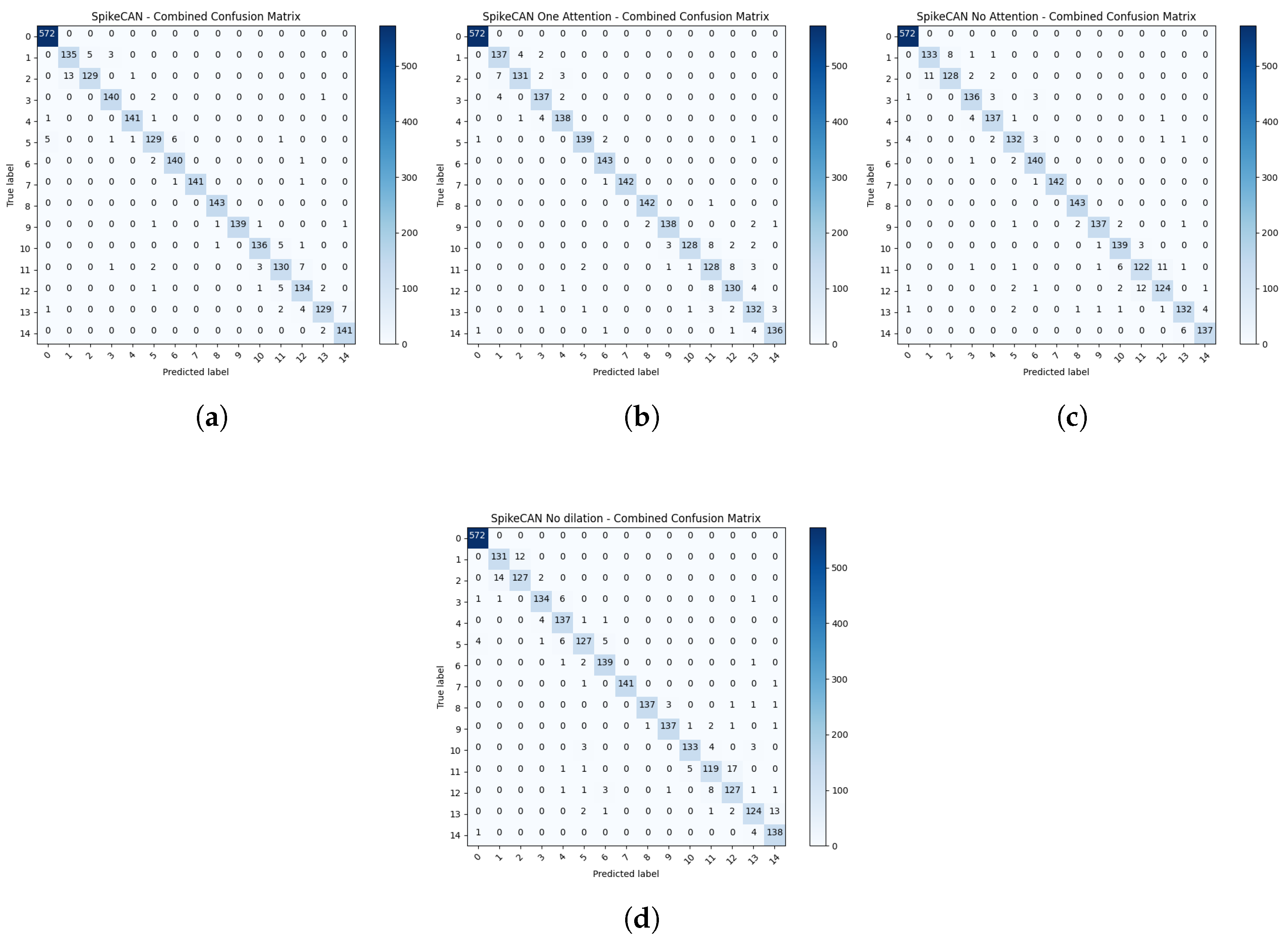
In our ablation study, we evaluated three modified versions of the original SpikeCAN model. The first variant, referred to as SpikeCAN with one attention module, retains only the first attention module while removing the second, allowing us to examine the marginal benefit of the second attention stage. The second variant, called SpikeCAN without attention modules, completely eliminates both SCA and STA blocks from the architecture. Finally, in the third variant, SpikeCAN without dilation, all dilated convolutions in the MDRF blocks are replaced with standard convolutions to assess the role of dilation in expanding temporal receptive fields.

The accuracies and F1 Scores for these ablation experiments are provided in

Table 5. Comparison of ablation methods.

Method	Without	Accuracy	F1 Score
SpikeCAN	-	96.31% ± 0.76%	0.9560
SpikeCAN One AM	Attention Module 2	96.08% ± 0.70%	0.9526
SpikeCAN No AM	Attention Module 1, 2	95.34% ± 0.57%	0.9436
SpikeCAN No dilation	dilation	94.09% ± 1.32%	0.9305

, and the corresponding confusion matrices are shown in Figure 6. The results clearly show that the full SpikeCAN model, with all modules intact, consistently achieves superior performance across all evaluation metrics. Notably, the confusion matrices reveal that the complete model maintains stable accuracy across all classes, including challenging cases such as Class 11 and Class 12. In contrast, the ablated variants exhibit increased misclassification in these classes, highlighting the effectiveness of the removed components.

Statistical analysis revealed that removing dilation from the SpikeCAN model resulted in a significant decrease in performance, with the accuracy reduced by approximately 2.22% (t = $2.8693$, $p=0.0209$) and the F1 Score decreased by about 0.0272 (t = $3.3938$, $p=0.0092$), highlighting the critical role of dilation in feature extraction. When examining the impact of removing attention modules, eliminating one attention module caused a slight performance drop compared to the original model, but this decrease was not statistically significant. However, removing both attention modules led to a marginally significant decrease in accuracy (t-statistic = $2.0669$, p = $0.0719$) and a statistically significant reduction in F1 Score (t-statistic = $3.3479$, p = $0.0099$), demonstrating the important contribution of attention mechanisms to the model’s performance.

These findings underscore the importance of both the attention mechanism and the dilated convolutional design in achieving high classification performance. The attention modules help focus on discriminative temporal and channel-wise features, while the use of dilation expands the receptive field without increasing computational cost. Together, they enable SpikeCAN to achieve robust and accurate diagnosis in complex fault scenarios.

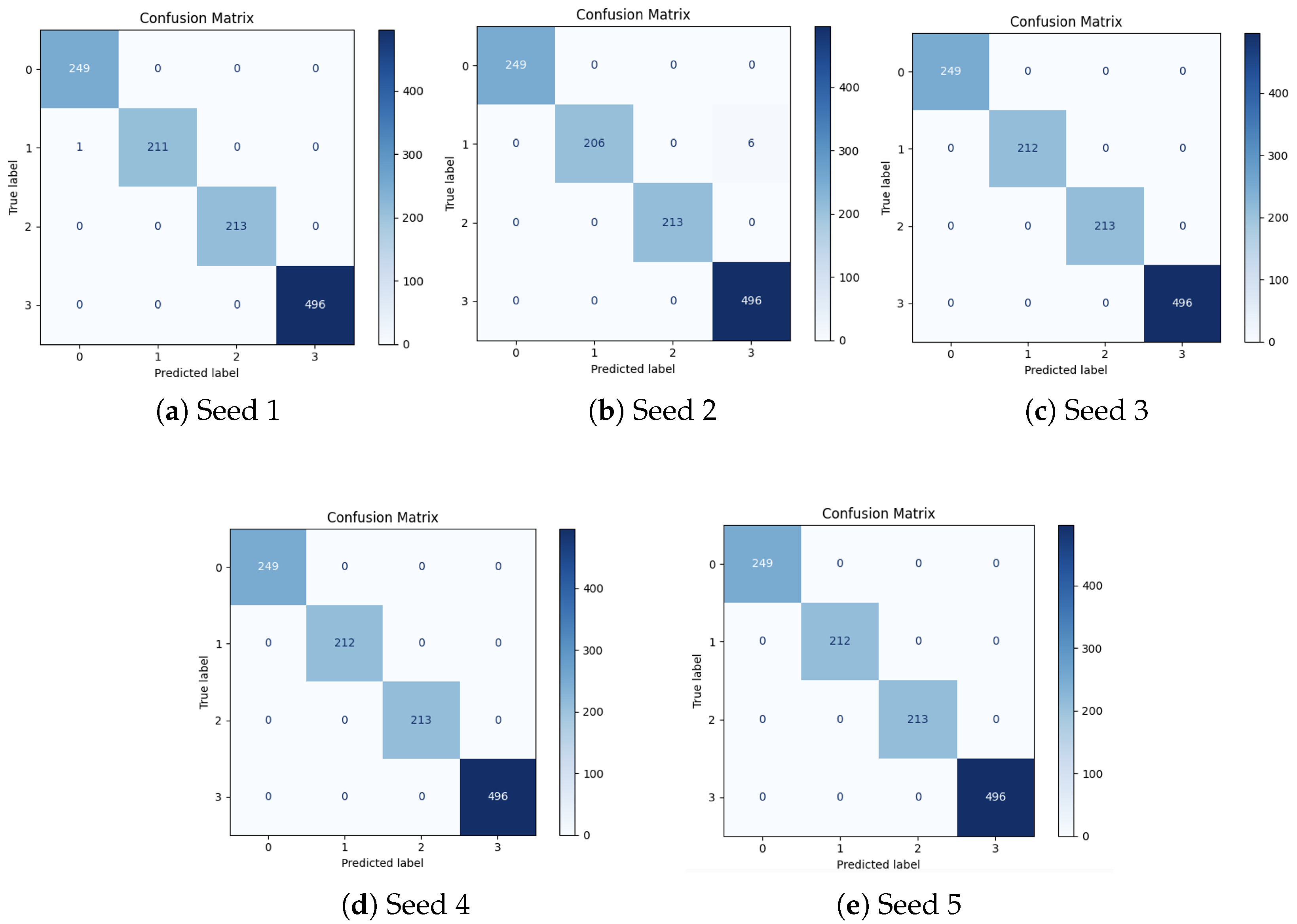
7.2. Robustness Analysis Under Varying Training Sample Sizes

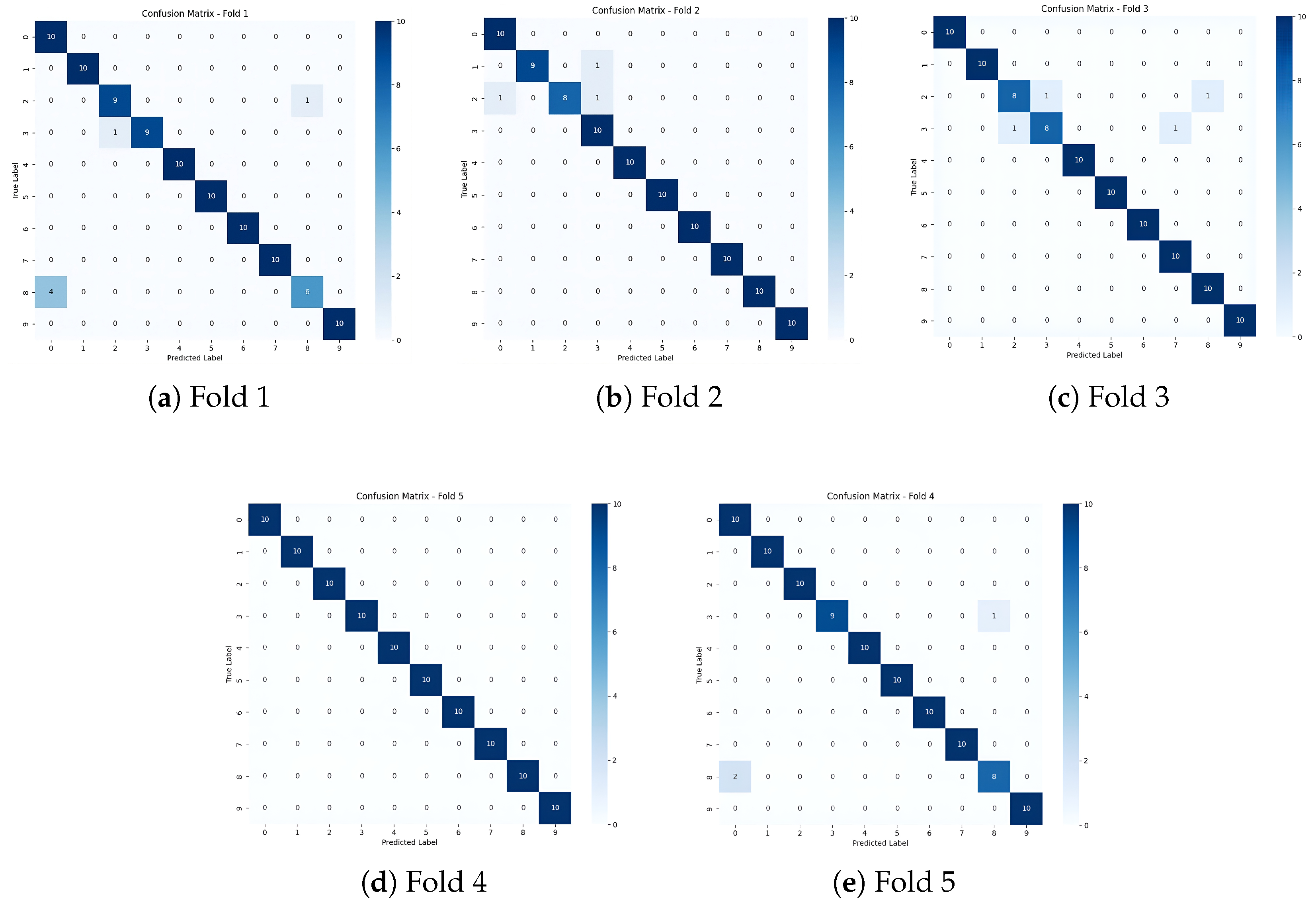
To assess the robustness of our SpikeCAN model with respect to the number of training samples per class presented in [47], we conducted experiments on the CWRU 10-class classification dataset. We systematically reduced the number of samples per class to 50, 40, and 30, and evaluated the model’s performance under each condition using five-fold cross-validation, summarized in

Table 6. Robustness analysis for CWRU 10-class classification with varying sample counts (50, 40, and 30 per class).

Sample Count	Accuracy (%)	F1 Score
50	97.80 ± 1.94	0.9674
40	89.73 ± 5.33	0.8827
30	78.33 ± 8.16	0.7555

.

Our results reveal that SpikeCAN maintains robust performance, with only a moderate decline in F1 Score of approximately 0.0847 when reducing the training samples from 50 to 40 per class, although this decrease is statistically significant (t-statistic = 2.9093, $p=0.0196$). This suggests that 40 samples per class can be a practical lower bound for reliable model training under the current experimental conditions. However, further reduction to 30 samples per class induces a pronounced degradation in performance, with an F1 Score drop of approximately 0.2119 relative to the 50-sample baseline (t-statistic = 5.9901, $p=0.0002$). Additionally, the difference in F1 Score between 40 and 30 samples per class is about 0.1272 (t-statistic = 2.8178, $p=0.0225$), reinforcing that the performance decline accelerates beyond the 40-sample threshold. These findings highlight an important trade-off between training data availability and diagnostic accuracy, emphasizing the necessity of sufficient sample sizes to ensure dependable fault diagnosis in practical industrial applications.

8. Discussion and Conclusions

The experimental evaluations conducted on the MFPT and CWRU datasets clearly demonstrate the substantial potential and practical utility of the proposed SpikeCAN model for industrial fault diagnosis tasks. On the MFPT dataset, SpikeCAN achieved a remarkable accuracy of 96.31% across a challenging 15-class classification scenario, while maintaining an exceptionally low theoretical energy consumption of 0.78 mJ per inference. Similarly, on the widely used CWRU dataset, SpikeCAN delivered robust classification performance, achieving 97.80% accuracy in a constrained data scenario (10-class) and 99.86% accuracy in a 4-class configuration, consuming only 3.71 mJ per inference. Furthermore, inference speed tests conducted on an RTX 4090 GPU indicate a processing time of approximately 27.49 ms per inference, underscoring SpikeCAN’s suitability for real-time monitoring tasks.

Beyond these promising quantitative results, SpikeCAN also presents important practical advantages that enhance its suitability for real-world industrial deployments. The inherent energy efficiency of its fully spike-driven architecture directly facilitates its application on resource-constrained edge devices, potentially leading to substantial reductions in operational costs and overall energy demands. Additionally, extensive experimental evaluations and comprehensive ablation studies have validated the robustness of SpikeCAN, highlighting its reliable and consistent performance across diverse fault conditions. Additional techniques, such as adaptive spike thresholding and data augmentation, could be effectively integrated to enhance robustness in real-world environments characterized by sensor noise and operational variability. SpikeCAN’s rapid inference capabilities, demonstrated empirically, also highlight its promise for timely fault detection and immediate corrective actions required in practical industrial monitoring scenarios.

Nevertheless, we acknowledge several practical limitations that must be considered when interpreting these results. Primarily, the reported energy consumption values are theoretical estimates derived from model operations, and fully realizing SpikeCAN’s low-energy advantages hinges critically upon the continued development and broader availability of specialized neuromorphic hardware designed specifically for spike-driven computation. Achieving optimal real-world performance on such hardware platforms will require substantial hardware-specific optimization of SpikeCAN, including dedicated encoding strategies for efficiently converting raw sensor data into spike signals. Additionally, practical challenges, such as dealing with data scarcity for rare fault conditions and managing noise and variability in industrial environments, must be carefully addressed in future developments and deployments.

Looking forward, several promising research opportunities emerge from this study. Extending SpikeCAN’s architecture to handle various types of industrial time-series signals beyond vibration data, including acoustic, electrical, and multi-modal sensor inputs, represents a compelling direction. Additionally, examining the interpretability of attention patterns learned by SpikeCAN, especially regarding their alignment with fault-relevant signal features, could provide valuable insights for enhanced diagnostic transparency and trustworthiness. Furthermore, integrating unsupervised or semi-supervised learning techniques could enable SpikeCAN to dynamically adapt to evolving operational conditions or previously unseen fault types without extensive labeled datasets.

In conclusion, this work introduced SpikeCAN, a fully spike-driven neural network architecture specifically designed to meet the rigorous demands of real-time and energy-efficient bearing fault diagnosis. By innovatively integrating spike-compatible channel and temporal attention mechanisms (SCA and STA) and multi-dilated receptive field convolutional structures (MDRF), SpikeCAN effectively extracts informative temporal features directly from raw sensor data with minimal computational overhead. The experimental results validate SpikeCAN’s state-of-the-art performance and significantly reduced theoretical energy requirements, highlighting its substantial potential for deployment in industrial IoT and edge computing scenarios. We anticipate that this study will stimulate further exploration into spike-driven architectures and contribute meaningfully toward the development of reliable, energy-aware, and robust real-time fault monitoring systems.

References

1. Gao, S.; Zhang, S.; Zhang, Y.; Gao, Y. Operational reliability evaluation and prediction of rolling bearing based on isometric mapping and NoCuSa-LSSVM. Reliab. Eng. Syst. Saf. 2020, 201, 106968. [Google Scholar] [CrossRef]
2. Zhou, Z.; Ai, Q.; Lou, P.; Hu, J.; Yan, J. A Novel Method for Rolling Bearing Fault Diagnosis Based on Gramian Angular Field and CNN-ViT. Sensors 2024, 24, 3967. [Google Scholar] [CrossRef]
3. Bonnett, A.H.; Yung, C. Increased Efficiency Versus Increased Reliability. IEEE Ind. Appl. Mag. 2008, 14, 29–36. [Google Scholar] [CrossRef]
4. Nandi, S.; Toliyat, H.A.; Li, X. Condition Monitoring and Fault Diagnosis of Electrical Motors—A Review. IEEE Trans. Energy Convers. 2005, 20, 719–729. [Google Scholar] [CrossRef]
5. Alonso-González, M.; Díaz, V.G.; Pérez, B.L.; G.-Bustelo, B.C.P.; Anzola, J.P. Bearing Fault Diagnosis With Envelope Analysis and Machine Learning Approaches Using CWRU Dataset. IEEE Access 2023, 11, 57796–57805. [Google Scholar] [CrossRef]
6. Huang, S.; Tang, J.; Dai, J.; Wang, Y. Signal Status Recognition Based on 1DCNN and Its Feature Extraction Mechanism Analysis. Sensors 2019, 19, 2018. [Google Scholar] [CrossRef] [PubMed]
7. Neupane, D.; Kim, Y.; Seok, J.; Hong, J. CNN-Based Fault Detection for Smart Manufacturing. Appl. Sci. 2021, 11, 11732. [Google Scholar] [CrossRef]
8. Zhang, Y.; Zhou, T.; Huang, X.; Cao, L.; Zhou, Q. Fault diagnosis of rotating machinery based on recurrent neural networks. Measurement 2021, 171, 108774. [Google Scholar] [CrossRef]
9. Jiang, H.; Li, X.; Shao, H.; Zhao, K. Intelligent fault diagnosis of rolling bearings using an improved deep recurrent neural network. Meas. Sci. Technol. 2018, 29, 065107. [Google Scholar] [CrossRef]
10. Vaswani, A.; Shazeer, N.; Parmar, N.; Uszkoreit, J.; Jones, L.; Gomez, A.N.; Kaiser, Ł.; Polosukhin, I. Attention is All You Need. In Proceedings of the 31st Conference on Neural Information Processing Systems (NIPS 2017), Long Beach, CA, USA, 4–9 December 2017; Volume 30. Available online: https://proceedings.neurips.cc/paper_files/paper/2017/file/3f5ee243547dee91fbd053c1c4a845aa-Paper.pdf (accessed on 1 March 2025).
11. Saeed, A.; Akram, M.U.; Khattak, M.; Khan, M.B. An interpretable hybrid framework combining convolution latent vectors with transformer based attention mechanism for rolling element fault detection and classification. Heliyon 2024, 10, e38993. [Google Scholar] [CrossRef]
12. Kitaev, N.; Kaiser, L.; Levskaya, A. Reformer: The Efficient Transformer. In Proceedings of the International Conference on Learning Representations (ICLR), Addis Ababa, Ethiopia, 30 April 2020; Available online: https://openreview.net/forum?id=rkgNKkHtvB (accessed on 1 March 2025).
13. Choromanski, K.M.; Likhosherstov, V.; Dohan, D.; Song, X.; Gane, A.; Sarlos, T.; Hawkins, P.; Davis, J.Q.; Mohiuddin, A.; Kaiser, L.; et al. Rethinking Attention with Performers. In Proceedings of the International Conference on Learning Representations (ICLR), Vienna, Austria, 4 May 2021; Available online: https://openreview.net/forum?id=Ua6zuk0WRH (accessed on 1 March 2025).
14. Zaheer, M.; Guruganesh, G.; Dubey, K.A.; Ainslie, J.; Alberti, C.; Ontanon, S.; Pham, P.; Ravula, A.; Wang, Q.; Yang, L.; et al. Big Bird: Transformers for Longer Sequences. In Proceedings of the 34th Conference on Neural Information Processing Systems (NeurIPS 2020), Vancouver, BC Canada, 6–12 December 2020; Volume 33, pp. 17283–17297. Available online: https://proceedings.neurips.cc/paper/2020/file/c8512d142a2d849725f31a9a7a361ab9-Paper.pdf (accessed on 1 March 2025).
15. Tay, Y.; Bahri, D.; Metzler, D.; Juan, D.-C.; Zhao, Z.; Zheng, C. Synthesizer: Rethinking Self-Attention in Transformer Models. arXiv 2020, arXiv:2005.00743. [Google Scholar]
16. Fu, L.; Yan, K.; Zhang, Y.; Chen, R.; Ma, Z.; Xu, F.; Zhu, T. EdgeCog: A Real-Time Bearing Fault Diagnosis System Based on Lightweight Edge Computing. IEEE Trans. Instrum. Meas. 2023, 72, 2521711. [Google Scholar] [CrossRef]
17. Maass, W. Networks of spiking neurons: The third generation of neural network models. Neural Netw. 1997, 10, 1659–1671. [Google Scholar] [CrossRef]
18. Yao, M.; Hu, J.; Zhou, Z.; Yuan, L.; Tian, Y.; XU, B.; Li, G. Spike-driven Transformer. In Proceedings of the Thirty-seventh Conference on Neural Information Processing Systems (NeurIPS), New Orleans, LA, USA, 10–16 December 2023; Available online: https://openreview.net/forum?id=9FmolyOHi5 (accessed on 1 March 2025).
19. Semenov, I.; Nikitin, D. Advantages and Disadvantages of Spiking Neural Networks Compared to Classical Artificial Neural Networks. In Proceedings of the 2023 Seminar on Information Computing and Processing (ICP), Saint Petersburg, Russia, 27–28 November 2023; pp. 192–194. [Google Scholar]
20. Zhang, H.; Li, Y.; He, B.; Fan, X.; Wang, Y.; Zhang, Y. Direct training high-performance spiking neural networks for object recognition and detection. Front. Neurosci. 2023, 17, 1229951. [Google Scholar] [CrossRef]
21. Gautrais, J.; Thorpe, S. Rate coding versus temporal order coding: A theoretical approach. Biosystems 1998, 48, 57–65. [Google Scholar] [CrossRef]
22. Comsa, I.M.; Potempa, K.; Versari, L.; Fischbacher, T.; Gesmundo, A.; Alakuijala, J. Temporal Coding in Spiking Neural Networks with Alpha Synaptic Function. In Proceedings of the ICASSP 2020—2020 IEEE International Conference on Acoustics, Speech and Signal Processing (ICASSP), Barcelona, Spain, 4–8 May 2020; pp. 8529–8533. [Google Scholar]
23. Wu, Y.; Deng, L.; Li, G.; Zhu, J.; Xie, Y.; Shi, L. Direct Training for Spiking Neural Networks: Faster, Larger, Better. In Proceedings of the AAAI Conference on Artificial Intelligence, Honolulu, HI, USA, 27 January–1 February 2019; Volume 33, pp. 1311–1318. [Google Scholar]
24. Kim, Y.; Park, H.; Moitra, A.; Bhattacharjee, A.; Venkatesha, Y.; Panda, P. Rate Coding Or Direct Coding: Which One Is Better For Accurate, Robust, Furthermore, Energy-Efficient Spiking Neural Networks? In Proceedings of the ICASSP 2022—2022 IEEE International Conference on Acoustics, Speech and Signal Processing (ICASSP), Singapore, 23–27 May 2022; pp. 71–75. [Google Scholar]
25. Neftci, E.O.; Mostafa, H.; Zenke, F. Surrogate Gradient Learning in Spiking Neural Networks: Bringing the Power of Gradient-based optimization to spiking neural networks. IEEE Signal Process. Mag. 2019, 36, 51–63. [Google Scholar] [CrossRef]
26. Fang, W.; Yu, Z.; Chen, Y.; Huang, T.; Masquelier, T.; Tian, Y. Deep Residual Learning in Spiking Neural Networks. In Proceedings of the NeurIPS 2021, Virtual, 6–14 December 2021; Volume 34, pp. 21056–21069. Available online: https://proceedings.neurips.cc/paper_files/paper/2021/file/afe434653a898da20044041262b3ac74-Paper.pdf (accessed on 1 March 2025).
27. Zhou, Z.; Zhu, Y.; He, C.; Wang, Y.; Yan, S.; Tian, Y.; Yuan, L. Spikformer: When Spiking Neural Network Meets Transformer. In Proceedings of the Eleventh International Conference on Learning Representations (ICLR), Kigali, Rwanda, 1–5 May 2023; Available online: https://openreview.net/forum?id=frE4fUwz_h (accessed on 1 March 2025).
28. Shi, X.; Hao, Z.; Yu, Z. SpikingResformer: Bridging ResNet and Vision Transformer in Spiking Neural Networks. In Proceedings of the 2024 IEEE/CVF Conference on Computer Vision and Pattern Recognition (CVPR), Seattle, WA, USA, 13–19 June 2024; pp. 5610–5619. [Google Scholar]
29. Smith, W.A.; Randall, R.B. Rolling element bearing diagnostics using the Case Western Reserve University data: A benchmark study. Mech. Syst. Signal Process. 2015, 64–65, 100–131. [Google Scholar] [CrossRef]
30. Machinery Failure Prevention Technology (MFPT). Available online: https://mfpt.org/fault-data-sets (accessed on 1 February 2025).
31. Fang, W.; Yu, Z.; Chen, Y.; Masquelier, T.; Huang, T.; Tian, Y. Incorporating learnable membrane time constant to enhance learning of spiking neural networks. In Proceedings of the 2021 IEEE/CVF International Conference on Computer Vision (ICCV), Montreal, BC, Canada, 11–17 October 2021; pp. 2641–2651. Available online: https://api.semanticscholar.org/CorpusID:226976144 (accessed on 1 March 2025).
32. Bu, T.; Fang, W.; Ding, J.; Dai, P.; Yu, Z.; Huang, T. Optimal ANN-SNN Conversion for High-accuracy and Ultra-low-latency Spiking Neural Networks. In Proceedings of the International Conference on Learning Representations (ICLR), Virtual, 25–29 April 2022; Available online: https://openreview.net/forum?id=7B3IJMM1k_M (accessed on 1 March 2025).
33. Yu, Q.; Tang, H.; Tan, K.C.; Yu, H. A brain-inspired spiking neural network model with temporal encoding and learning. Neurocomputing 2014, 138, 3–13. [Google Scholar] [CrossRef]
34. Zuo, L.; Xu, F.; Zhang, C.; Xiahou, T.; Liu, Y. A multi-layer spiking neural network-based approach to bearing fault diagnosis. Reliab. Eng. Syst. Saf. 2022, 225, 108561. [Google Scholar] [CrossRef]
35. Zuo, L.; Zhang, L.; Zhang, Z.-H.; Luo, X.-L.; Liu, Y. A spiking neural network-based approach to bearing fault diagnosis. J. Manuf. Syst. 2021, 61, 714–724. [Google Scholar] [CrossRef]
36. Woo, S.; Park, J.; Lee, J.-Y.; Kweon, I.S. CBAM: Convolutional Block Attention Module. In Proceedings of the European Conference on Computer Vision (ECCV), Munich, Germany, 8–14 September 2018; Volume 11211, pp. 3–19. [Google Scholar]
37. Yang, Y.; Long, Y.; Lin, Y.; Gao, Z.; Rui, L.; Yu, P. Two-stage edge-side fault diagnosis method based on double knowledge distillation. Comput. Mater. Contin. 2023, 76, 3623–3651. [Google Scholar] [CrossRef]
38. He, K.; Zhang, X.; Ren, S.; Sun, J. Deep Residual Learning for Image Recognition. In Proceedings of the IEEE Conference on Computer Vision and Pattern Recognition (CVPR), Las Vegas, NV, USA, 27–30 June 2016; pp. 770–778. Available online: https://openaccess.thecvf.com/content_cvpr_2016/html/He_Deep_Residual_Learning_CVPR_2016_paper.html (accessed on 1 March 2025).
39. Sengupta, A.; Ye, Y.; Wang, R.; Liu, C.; Roy, K. Going Deeper in Spiking Neural Networks: VGG and Residual Architectures. Front. Neurosci. 2019, 13, 95. [Google Scholar] [CrossRef]
40. Wang, Z.; Yao, L.; Chen, G.; Ding, J. Modified multiscale weighted permutation entropy and optimized support vector machine method for rolling bearing fault diagnosis with complex signals. ISA Trans. 2021, 114, 470–484. [Google Scholar] [CrossRef]
41. Muruganatham, B.; Sanjith, M.A.; Krishnakumar, B.; Murty, S.A.V.S. Roller element bearing fault diagnosis using singular spectrum analysis. Mech. Syst. Signal Process. 2013, 35, 150–166. [Google Scholar] [CrossRef]
42. Pan, J.; Zi, Y.; Chen, J.; Zhou, Z.; Wang, B. LiftingNet: A Novel Deep Learning Network With Layerwise Feature Learning From Noisy Mechanical Data for Fault Classification. IEEE Trans. Ind. Electron. 2018, 65, 4973–4982. [Google Scholar] [CrossRef]
43. Wang, S.; Xiang, J.; Zhong, Y.; Zhou, Y. Convolutional neural network-based hidden Markov models for rolling element bearing fault identification. Knowl.-Based Syst. 2018, 144, 65–76. [Google Scholar] [CrossRef]
44. Li, H.; Huang, J.; Ji, S. Bearing Fault Diagnosis with a Feature Fusion Method Based on an Ensemble Convolutional Neural Network and Deep Neural Network. Sensors 2019, 19, 2034. [Google Scholar] [CrossRef] [PubMed]
45. Han, K.; Wang, W.; Guo, J. Research on a Bearing Fault Diagnosis Method Based on a CNN-LSTM-GRU Model. Machines 2024, 12, 927. [Google Scholar] [CrossRef]
46. Magar, R.; Ghule, L.; Li, J.; Zhao, Y.; Farimani, A.B. FaultNet: A Deep Convolutional Neural Network for Bearing Fault Classification. IEEE Access 2021, 9, 25189–25199. [Google Scholar] [CrossRef]
47. van den Hoogen, J.; Bloemheuvel, S.; Atzmueller, M. Classifying Multivariate Signals in Rolling Bearing Fault Detection Using Adaptive Wide-Kernel CNNs. Appl. Sci. 2021, 11, 11429. [Google Scholar] [CrossRef]
Figure 1. Overall architecture of the proposed SpikeCAN.
Applsci 15 07622 g001
Figure 2. The overall architecture of Spike Convolutional Attention.
Applsci 15 07622 g002
Figure 3. Confusion matrices illustrating the classification performance on MFPT.
Applsci 15 07622 g003
Figure 4. Confusion matrices illustrating the classification performance on CWRU.
Applsci 15 07622 g004
Figure 5. Confusion matrices illustrating the classification performance on the CWRU dataset (50 samples per class).
Applsci 15 07622 g005
Figure 6. Confusion matrices illustrating the classification performance across different ablation scenarios compared with the original SpikeCAN model. (a) SpikeCAN. (b) SpikeCAN One Attention block. (c) SpikeCAN No Attention block. (d) SpikeCAN No dilation.
Applsci 15 07622 g006