Ground-Level Surface Reconstruction and Soil Volume Estimation in Construction Sites Using Marching Cubes Method

Abstract

Accurate environmental sensing is pivotal for advancing automation in construction, particularly in autonomous excavation. Precise 3D representations of complex and dynamic site geometries is essential for obstacle detection, progress monitoring, and safe operation. However, existing sensing techniques often struggle with capturing irregular surfaces and incomplete data in real-time, leading to significant challenges in practical deployment. To address these gaps, we present a novel framework integrating curve approximation, surface reconstruction, and marching cubes algorithm to transform raw sensor data into a detailed and computationally efficient soil surface representation. Our approach improves site modeling accuracy, paving the way for reliable and efficient construction automation. This paper enhances sensory data quality using surface reconstruction techniques, followed by the marching cubes algorithm to generate an accurate and flexible 3D soil model. This model facilitates rapid estimation of soil volume, weight, and shape, offering an efficient approach for environmental analysis and decision-making in automated systems. Experimental validation demonstrated the effectiveness of the proposed method, achieving relative errors of 4.92% and 1.42% across two excavation cycles. Additionally, the marching cubes algorithm completed volume estimation in just 0.05 s, confirming the approach’s accuracy and suitability for real-time applications in dynamic construction environments.

1. Introduction

Accurate ground surface reconstruction and soil volume estimation are essential for modern construction site management, underpinning precise planning, efficient resource allocation, and the effective monitoring of excavation activities. These processes are increasingly critical in the context of autonomous excavation in construction sites, where systems depend on sensory data to perceive and interact with their environments. Despite substantial advancements in sensor technology, significant challenges remain in harnessing raw sensor data effectively for high-fidelity surface modeling and precise soil volume estimation in digging areas.

Sensors such as depth cameras, commonly employed to capture site data, often produce noisy, incomplete, or inconsistent measurements, limiting their utility in creating accurate surface models and volume calculations. Noise, invalid pixels, and outliers in raw sensor data can significantly distort ground surface representations, introducing inaccuracies in subsequent computations. Traditional surface reconstruction and volume estimation methods often struggle with these data quality issues. Many rely on computationally intensive algorithms unsuitable for real-time applications, particularly in dynamic environments like construction sites. Additionally, these methods frequently lack the robustness to handle the inherent uncertainties in sensory data, leading to unreliable outputs that undermine their suitability for automation and decision-making tasks.

A major limitation in existing approaches lies in their inability to effectively bridge the gap between raw sensor data and actionable metrics [1,2,3,4,5,6]. Raw data, while providing a snapshot of the environment, often yield suboptimal results when directly applied to algorithms for tasks such as volume and mass estimation. Without robust preprocessing and advanced modeling techniques, this data remains insufficient for generating the precise and reliable information required for autonomous operations and effective site management.

This study addresses these challenges by proposing a novel methodology that integrates curve approximation techniques with the marching cubes algorithm to achieve accurate ground surface reconstruction and soil volume estimation. The approach transforms pixelated depth data into smooth, continuous surface representations, effectively mitigating the challenges resulting from imprecise sensor data and unexpected deviations.

By approximating raw sensor data using analytical equations, the method ensures accuracy and continuity in surface modeling, making it suitable for the dynamic and complex conditions of construction sites.

In addition, the marching cubes algorithm is a cornerstone of the proposed framework, enabling the conversion of reconstructed surfaces into volumetric representations. This facilitates the efficient calculation of critical soil metrics such as volume and mass, supporting excavation monitoring and operational planning. Computational efficiency is a key focus, with the method leveraging parallelization to deliver low-latency performance while maintaining robustness against uncertainties in sensory data.

The primary objective of this study is to provide a scalable, accurate, and efficient solution for surface reconstruction and volume estimation tailored to the demands of autonomous excavation and construction site management. By addressing the challenges posed by noisy and inconsistent sensory data, the proposed methodology represents a significant improvement over traditional approaches. Specifically, it not only enhances the accuracy and reliability of extracted metrics but also reduces computational cost, making it practical for deployment in automated systems.

Experimental validation demonstrates the effectiveness of the proposed methodology during the excavation process. The results illustrate its capability to transform raw depth data collected by depth cameras into actionable insights. This advancement enhances the integration of digging cycle planning and monitoring in common excavator applications, including digging, trenching, and leveling. This study thus lays the foundation for incorporating advanced computational techniques into site management, delivering improvements in efficiency, accuracy, and innovation across the construction industry.

2. Literature Review

Accurate surface reconstruction and soil volume estimation are essential components of construction site management and autonomous excavation systems. The challenges of handling noisy data, computational efficiency, and accuracy have been extensively studied. This section reviews methods and advancements in surface reconstruction, volume estimation, and applications in construction automation.

2.1. Surface Reconstruction Techniques

Surface reconstruction is a critical process in converting raw sensor data into usable terrain models. Early methods, such as the work of Hoppe et al. [1], introduced algorithms for reconstructing surfaces from unorganized points. Curless and Levoy [2] proposed volumetric approaches that leveraged signed distance fields to create accurate models. Kazhdan et al. [3] advanced this with Poisson surface reconstruction, offering improved robustness against noise but at a high computational cost.

In the study of Alexa et al. [7], point set surfaces utilized Moving Least Squares (MLS) for smooth reconstructions but struggled in dynamic environments. Real-time methods like KinectFusion [4] and its derivatives [8] combined depth sensors with GPU acceleration for rapid reconstruction. Dai et al. [5] further enhanced real-time 3D reconstruction with BundleFusion, which ensured globally consistent surface maps in dynamic scenes.

Techniques like DeepVoxels [6] and Neural Radiance Fields (NeRF) [9] have recently leveraged neural networks to model surfaces, though they remain computationally intensive for real-time applications. Fusion-based methods [10] and implicit representation techniques [11] offer promising directions for integrating machine learning into reconstruction pipelines.

2.2. Volume Estimation Methods

Volume estimation has significant applications in geoscience and construction. Traditional methods, including manual surveying [12] and photogrammetry [13], provided reliable but labor-intensive results. The advent of LiDAR [13] offered high accuracy but incurred high costs.

Algorithmic approaches like the marching cubes algorithm [14] transformed scalar fields into volumetric models. The marching cubes algorithm is mainly used in the health industry to convert the layered images obtained during the computed tomography (CT) and magnetic resonance (MR) scans into a 3D volumetric representation. Enhancements by Montani et al. [8] improved the handling of ambiguous cases. Adaptive marching cubes [14] introduced further computational optimizations but required preprocessing. Dual contouring methods [15] provided higher accuracy in regions with sharp features.

2.3. Handling Sensor Noise and Data Gaps

Sensor noise significantly impacts reconstruction accuracy. Bilateral filtering [12] and robust regression [16] have been employed to preprocess data. More recent studies by Zhang et al. [17] and Sun et al. [16] utilized deep learning for denoising, achieving notable improvements. Various approaches, such as filter-based, optimization-based, and deep learning-based algorithms, are used to enhance the quality of depth images and 3D point clouds. Filter-based methods aim to reduce noise using principles of image processing. Optimization-based approaches minimize noise by applying optimization algorithms to find an optimal point cloud that best fits the noisy data while satisfying specific criteria. Deep learning-based techniques train models using noisy point cloud data and their corresponding ground truth to improve accuracy.

Outlier removal techniques, including RANSAC [18] and statistical outlier filtering [19], have been integrated into reconstruction pipelines. Curve approximation methods, such as splines [20] and B-splines [21], offer smooth representations of scattered data. However, they are most commonly used in computer graphic applications. In this study, the curve approximation is applied for terrain surface modeling. The use of robust statistical methods [22] and Gaussian processes [23] has further enhanced data reliability.

2.4. Recent Advancments

Several recent methods have achieved real-time or near-real-time surface reconstruction using learning-based techniques, yet they remain unsuitable for dynamic excavation environments. NeuralRecon reconstructs 3D geometry from monocular video by fusing depth across sequential frames, but it assumes a static scene and smooth camera motion—conditions rarely met during excavation, where the geometry changes abruptly [24]. Co-SLAM combines neural representations with traditional SLAM for high-fidelity RGB-D mapping, but it also depends on temporal consistency and static backgrounds, making it vulnerable to occlusions and terrain changes typical of excavation [25]. Meanwhile, Neural Surface Reconstruction of Dynamic Scenes models non-rigid deformation from RGB-D input, but its computational cost and sensitivity to topological changes limit its ability to capture the fast, discontinuous transformations of soil and debris [26]. These methods, though advanced, are not designed for single-shot, real-time volumetric reconstruction in highly dynamic, unstructured outdoor settings.

2.5. Research Gaps and Contributions

Despite the research progress made in [1,2,3,4,5,6,7,8,9,10,11], key gaps remain in effectively addressing noisy and incomplete data, in addition to high computational costs. Many traditional methods lack scalability and real-time capability. Drawing from our literature review, conventional curve approximation techniques, such as splines [20] and B-splines [21], have primarily been applied in computer graphics, rather than for terrain modeling. In contrast, our study repurposes these methods for robust terrain surface approximation under noisy conditions, which is critical for construction site management. Similarly, traditional implementations of the marching cubes algorithm [14] have been extensively used in static medical imaging but not in dynamic, large scale excavation site. Our integrated approach refines the marching cubes process for real-time volumetric reconstruction and soil volume estimation, offering a scalable and efficient solution tailored to autonomous excavation systems.

3. Methodology

This section provides a detailed explanation of the proposed method for addressing the gaps identified in Section 1.

The first step toward achieving autonomous excavation is to accurately identify the surrounding environment. In this study, a depth camera is strategically positioned to monitor the excavation area. The camera captures and reports depth information. However, as with any sensor, the cameras are prone to errors, occasionally producing invalid data. Consequently, it is necessary to filter out such data to generate precise and reliable information.

Raw data from the camera often contain invalid pixels and outliers, necessitating refinement. To address this, the pixelated data are converted into analytical representations. This approach provides two key advantages: enabling data interpolation and reconstruction of soil surface. Detailed discussions of these processes are provided in Section 3.3 and Section 3.4, respectively. Section 3.5 includes the marching cubes approach used for soil volume estimation.

The proposed methodology introduces several enhancements aimed at increasing the accuracy of construction site modeling, particularly by refining raw sensor data and enabling detailed surface reconstruction. A key improvement involves filtering and transforming depth camera outputs, which are often noisy and contain invalid or missing pixels. By converting these raw, pixelated measurements into analytical representations using curve approximation techniques, the method allows for continuous interpolation across the excavation area. This process ensures that even unsampled points between pixels can be accurately estimated, significantly enhancing the resolution and completeness of the surface model.

To further improve modeling fidelity, the methodology emphasizes continuity in the interpolated data. Soil surfaces are naturally smooth and lack abrupt geometric changes; therefore, the algorithm imposes $C^0$ and $c^1$ continuity constraints on the fitted splines. Each image row is treated as a signal and approximated using third-degree polynomial splines, with coefficients optimized through the Levenberg–Marquardt algorithm. This eliminates abrupt transitions and outliers, producing a coherent and realistic representation of the terrain that is better suited for autonomous excavation tasks.

Additionally, the approach extends beyond interpolation to construct a complete and hole-free 3D surface. Using the analytical curves, the surface is densely reconstructed by connecting interpolated points into quads, preserving the spatial relationships captured in the depth image. The marching cubes algorithm is then applied to this surface for accurate volume estimation, leveraging precomputed templates to ensure both efficiency and consistency. This deterministic pipeline, free from random optimization processes, ensures repeatable and high-fidelity modeling results, effectively addressing the challenges of data noise, continuity, and volumetric precision in excavation environments.

3.1. Interpolation

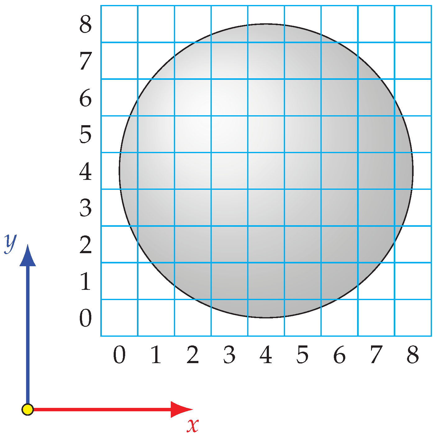
Each frame captured by the camera generates a depth image, where each pixel corresponds to a sampled value. These sampled values form a set of scattered data points. To accurately reconstruct the 3D shape of the excavation area, it is essential to transform these scattered points into a mathematical model that can represent the surface at any location.

Each pixel, illustrated in Figure 1, in the image taken from Figure 2 is associated with two integer values representing its position $(x,y)$ in pixel coordinate frame and a measured value representing the sampled data. For instance, in the depth image, the measured value corresponds to the distance between the camera and the object’s surface at that location.

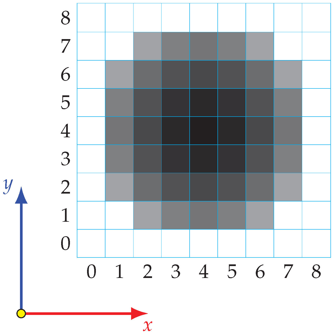
As shown in Figure 3, each pixel’s measured value represents the distance between the camera and the object’s surface. These values are visually represented in shades of gray, with black and white denoting the minimum and maximum distances, respectively. Since data are captured only at integer pixel positions, intermediate values between neighboring pixels are absent. To address this, a curve approximation algorithm is applied to transform scattered data into an analytical equation, allowing interpolation at any coordinate (x, y).

3.2. Continuity

Captured data often deviate from ground truth due to factors such as external infrared light sources, reflections, particulates, and sensor imperfections. These issues result in invalid data and outliers that disrupt the coherence of depth images.

Outliers are particularly problematic, as the soil does not exhibit sharp, isolated points distant from other points in the point cloud. Thus, points that significantly deviate from their neighbors are identified as outliers and filtered out. Enhancing the continuity of data is essential for accurately reconstructing the excavation area. Due to the inherent characteristics of soil, its surface tends to be smooth with minimal sharp edges. Therefore, enforcing continuity in the reconstruction process allows the simulated soil surface to better retain its original shape, leading to a more accurate representation of real-world data.

3.3. Curve Approximation

To simultaneously address interpolation and continuity, a curve approximation algorithm is proposed. This approach generates a smooth mathematical representation of the data, eliminating outliers and enabling evaluation at any point. Each row of the depth image is treated as an independent signal, where the x-axis represents the pixel position and the z-axis corresponds to the depth value. Figure 4 illustrates the fifth row of Figure 3 and its approximated curve.

To approximate signals, a third-degree polynomial spline is chosen as the mathematical model, ensuring both smoothness and computational efficiency. The equations and continuity constraints for the spline are detailed in Equations (1)–(7). The coefficients of the spline are optimized using the Levenberg–Marquardt algorithm (LMA) to minimize the error defined in Equation (8).

$$P:[0,w-1]\to \mathbb{R}$$

(1)

The width of the image, denoted as w, represents the number of pixels in each row.

$$\mathbf{t}=\{[t_0,\dots ,t_k]:t_i\le t_{i+1}\forall i=0,\dots ,k-1\}$$

(2)

The knot vector $\mathbf{t}$ is used in this study with $k=10$, and it is uniformly distributed along the range $[0,w-1]$. Thus, each knot value $t_i$ is defined as $t_i={\displaystyle \frac{i(w-1)}{10}}$, where i ranges from 0 to 10, w is the width of image in pixels, and k is number of knot vectors.

$$[0,w-1]=[t_0,t_1)\cup [t_1,t_2)\cup \dots \cup [t_{k-2},t_{k-1})\cup [t_{k-1},t_k]$$

(3)

In this study, the knot vector $\mathbf{t}$ is defined as $\mathbf{t}=[0,{\displaystyle \frac{(w-1)}{10}},{\displaystyle \frac{2(w-1)}{10}},\dots ,{\displaystyle \frac{9(w-1)}{10}},w-1]$.

$$P\left(t\right)=\left\{\begin{array}{c}{P}_0\left(t\right),t_0\le t<t_1\hfill \\ P_1\left(t\right),t_1\le t<t_2\hfill \\ ⋮\hfill \\ P_{k-1}\left(t\right),t_{k-1}\le t\le t_k\hfill \end{array}\right.$$

(4)

Equation (4) determines the equation based on the span to which t belongs in $\mathbf{t}$.

$$P_i\left(t\right)=\sum _{j=0}^n{a}_{i,j}{t}^j$$

(5)

The polynomial equation of the defined curve is given by Equation (5). For this study, a cubic polynomial curve is formed with $n=2$, so $P_i\left(t\right)=a_{i,0}+a_{i,1}{t}_i+a_{i,2}{t}_i^2$ where $a_{i,j}$ denotes the coefficient associated with the j-th power of t for the i-th curve.

$$P_i\left(t_{i+1}\right)=P_{i+1}\left(t_{i+1}\right)i=0,\dots ,k-1$$

(6)

$${\displaystyle \frac{d{P}_i}{dt}}\left(t_{i+1}\right)={\displaystyle \frac{d{P}_{i+1}}{dt}}\left(t_{i+1}\right)i=0,\dots ,k-1$$

(7)

Continuity criteria applied to splines are defined in Equations (6) and (7). Equation (6) ensures $C^0$ continuity by connecting the curves at the knot vector locations. Additionally, Equation (7) guarantees $C^1$ continuity, which means that there are no sharp points at the knot vector locations.

To approximate this signal, the unknown variables are the coefficients $a_{i,j}$ in Equation (5). Since the equations are non-linear, the LMA is chosen for curve approximation to minimize the deviation between the approximated curve and the initial input data.

$$e=\sum _{i=0}^{w-1}{(z_i-P_i\left(t_i\right))}^2$$

(8)

In Equation (8), $z_i$ represents the discrete data, and $P\left(i\right)$ represents the approximated curve at the same position i as $z_i$.

The deviation, denoted as e, is the quantity that needs to be minimized. The LMA is an iterative method and requires an initial value. In this study, the initial values are set as a vector with value of 1, and the iteration continues until a certain threshold is reached.

3.4. Surface Reconstruction

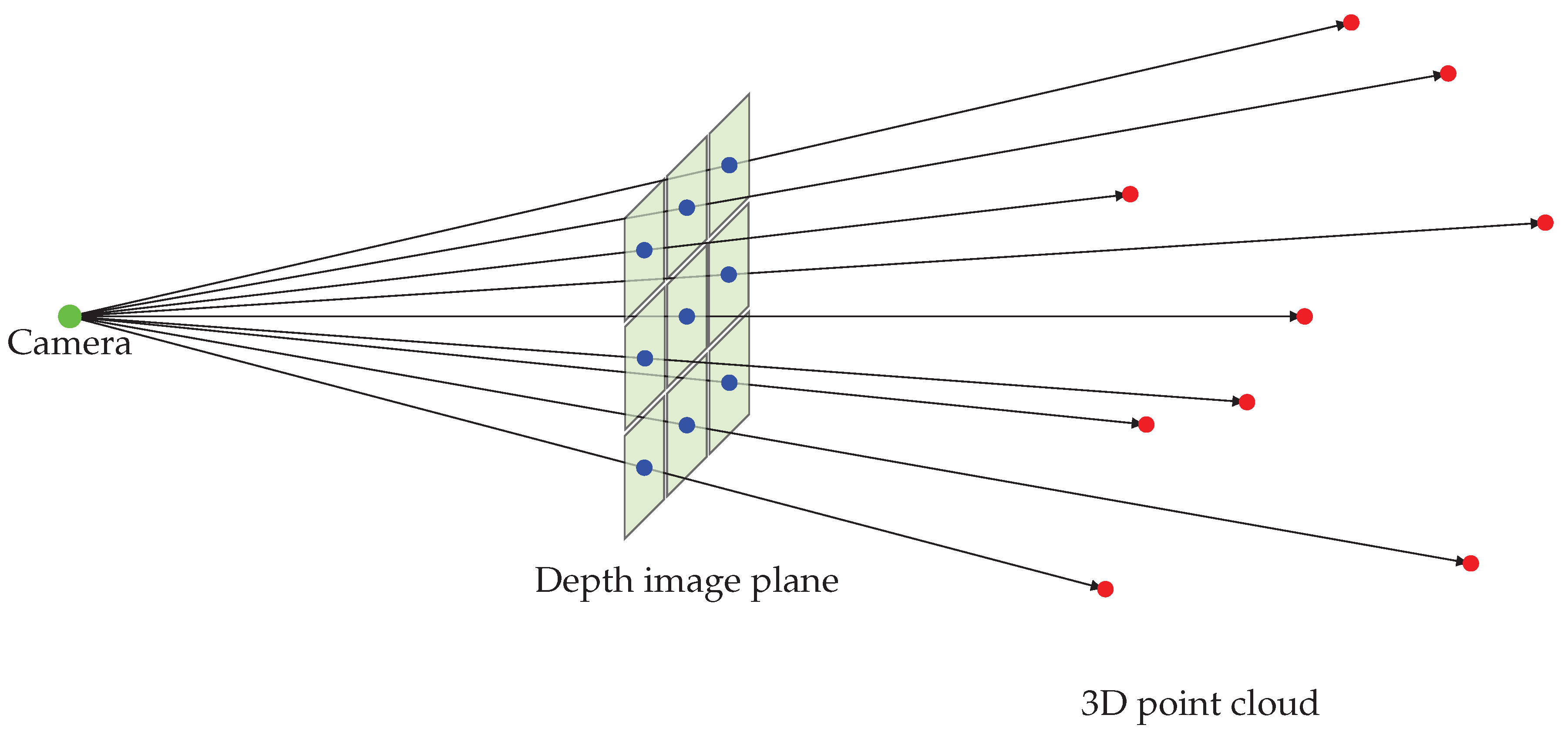
After approximating each row of the depth image as a curve, it becomes possible to evaluate the surface value at any given point. To assess the surface at coordinates (x, y), the first step is to determine the two neighboring rows of the depth image using Equation (10). The deprojection of the 3D point cloud into the depth image is shown in Figure 5.

$$y=\{y\in \mathbb{R}\mid 0\le y\le h\}$$

(9)

Here, h represents the height of the depth image.

$$j=\lfloor y\rfloor$$

(10)

The point at (x, y) lies between the j-th and $(j+1)$-th rows of the depth image. Consequently, the values of the approximated curves for these two rows are evaluated at position x. A linear interpolation is then performed between the two estimated values to obtain the interpolated measured value r at the specified point (x, y). Therefore, the interpolated value of the depth image at any given point (x, y) can be obtained using Equation (11).

$$r(x,y)=r_j\left(x\right)+(y-j)(r_{j+1}\left(x\right)-r_j\left(x\right))$$

(11)

Hence, the evaluation of the scatter depth image captured by a depth camera can be performed at any desired resolution, ensuring that outliers and invalid data are not a concern.

Although the interpolated data exists in the depth image space, it needs to be transformed into (x, y, z) space to represent a 3D point cloud for further utilization. To achieve this transformation, a mapping function provided by the manufacturer of the depth camera is employed.

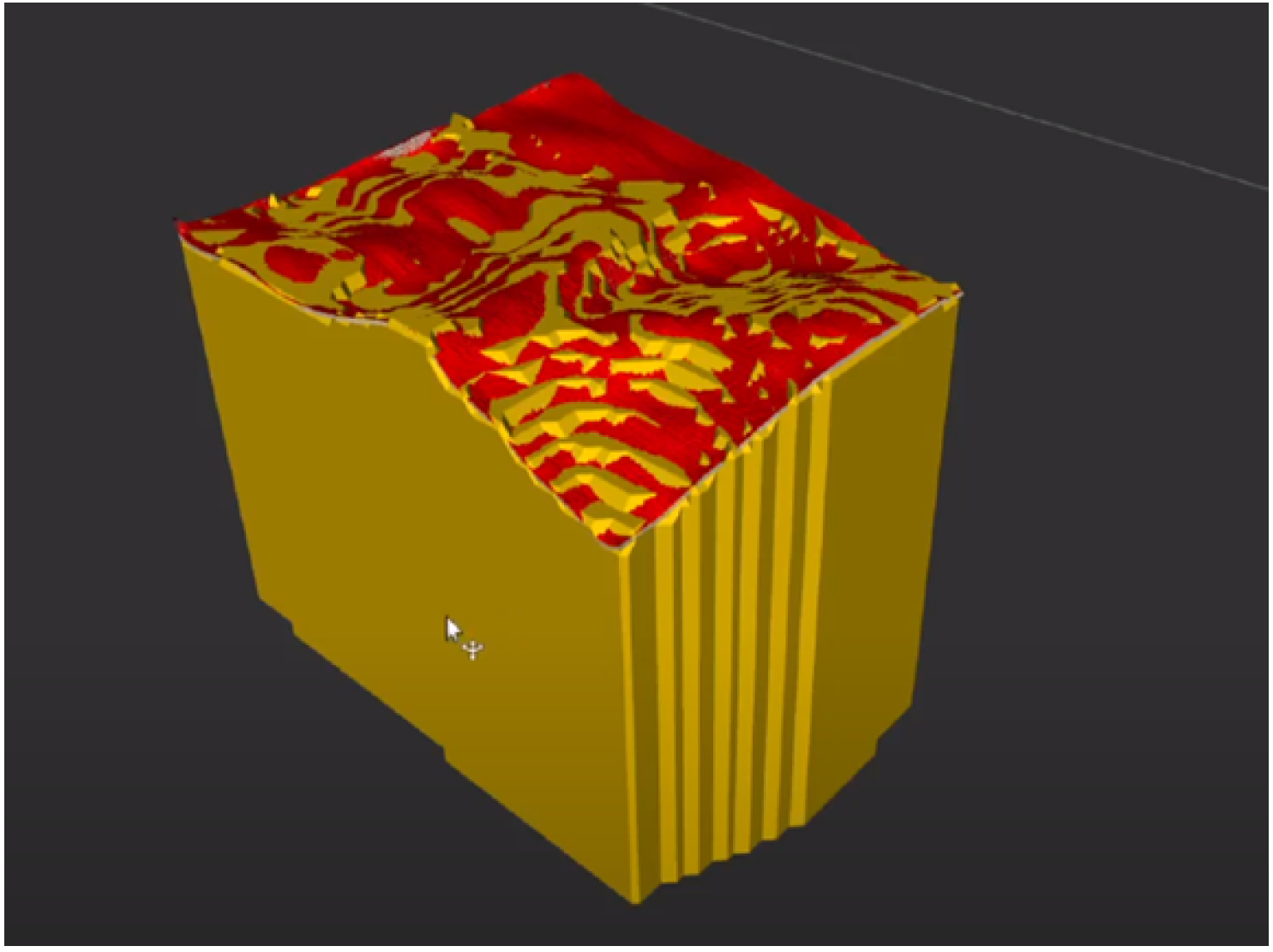
Subsequently, the points must be connected to form a cohesive surface. Each pixel in the depth image corresponds to a point in the 3D point cloud, and the connectivity data between neighboring points is preserved from the depth image. Consequently, it is possible to identify neighboring points in the depth image and establish a quad in 3D space. It is worth noting that the pixels (i, j), ($i+1$, j), ($i+1$, $j+1$), and (i, $j+1$) constitute a rectangle in the depth image. Consequently, their representation in the 3D point cloud also forms a quad in the same sequential order. By combining these quads, a continuous and hole-free surface of the area captured by the depth camera is constructed, effectively representing the shape of the soil in the excavation area as shown in Figure 6.

The proposed method offers a high-speed approach to surface reconstruction as it operates without the need for optimization. Moreover, it is reliable and deterministic, relying solely on a series of mathematical formulas rather than random numbers for optimization. Consequently, it consistently produces the same results for a given input. Additionally, it guarantees that the generated surface is free of holes, which is a crucial characteristic of this surface reconstruction approach.

3.5. Marching Cubes

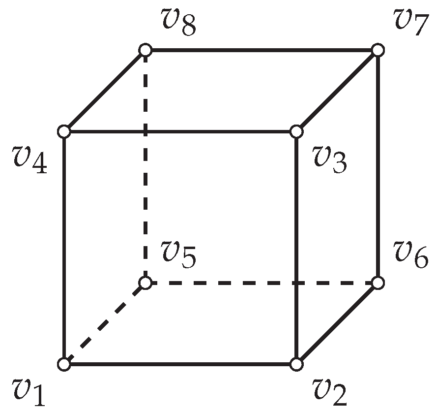
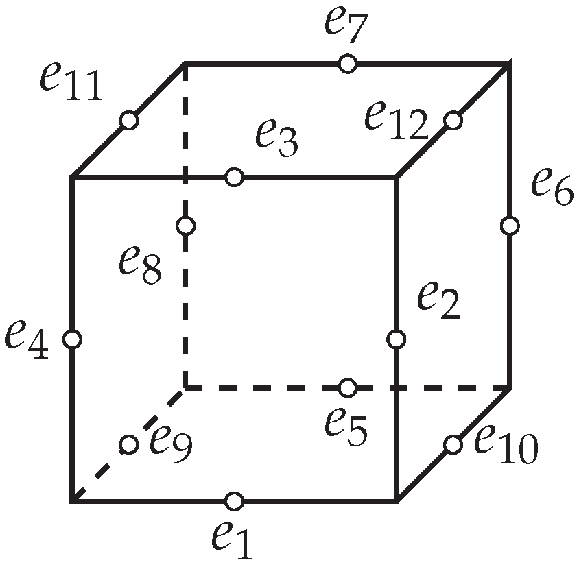
The surface reconstruction generates a mathematical model that the marching cubes algorithm can utilize to estimate the soil volume in the excavation area. Each marching cube consists of eight vertices and twelve edges, as shown in Figure 7 and Figure 8 from [14], respectively. Figure 9 illustrates the vertex indexing scheme for a single marching cube, also adapted from [14].

The marching cubes algorithm employs a three-dimensional discrete scalar field to extract a 3D mesh from an iso-surface. In this particular case, the iso-surface is constructed from the surface reconstruction detailed in Section 3.4. Each vertex includes a Boolean value that indicates whether it lies inside the soil or not. The z coordinate of the reconstructed surface is calculated at the same (x, y) coordinates of the vertex. If the z value of the vertex is lower than that of the reconstructed surface, it signifies that the vertex lies below the soil surface.

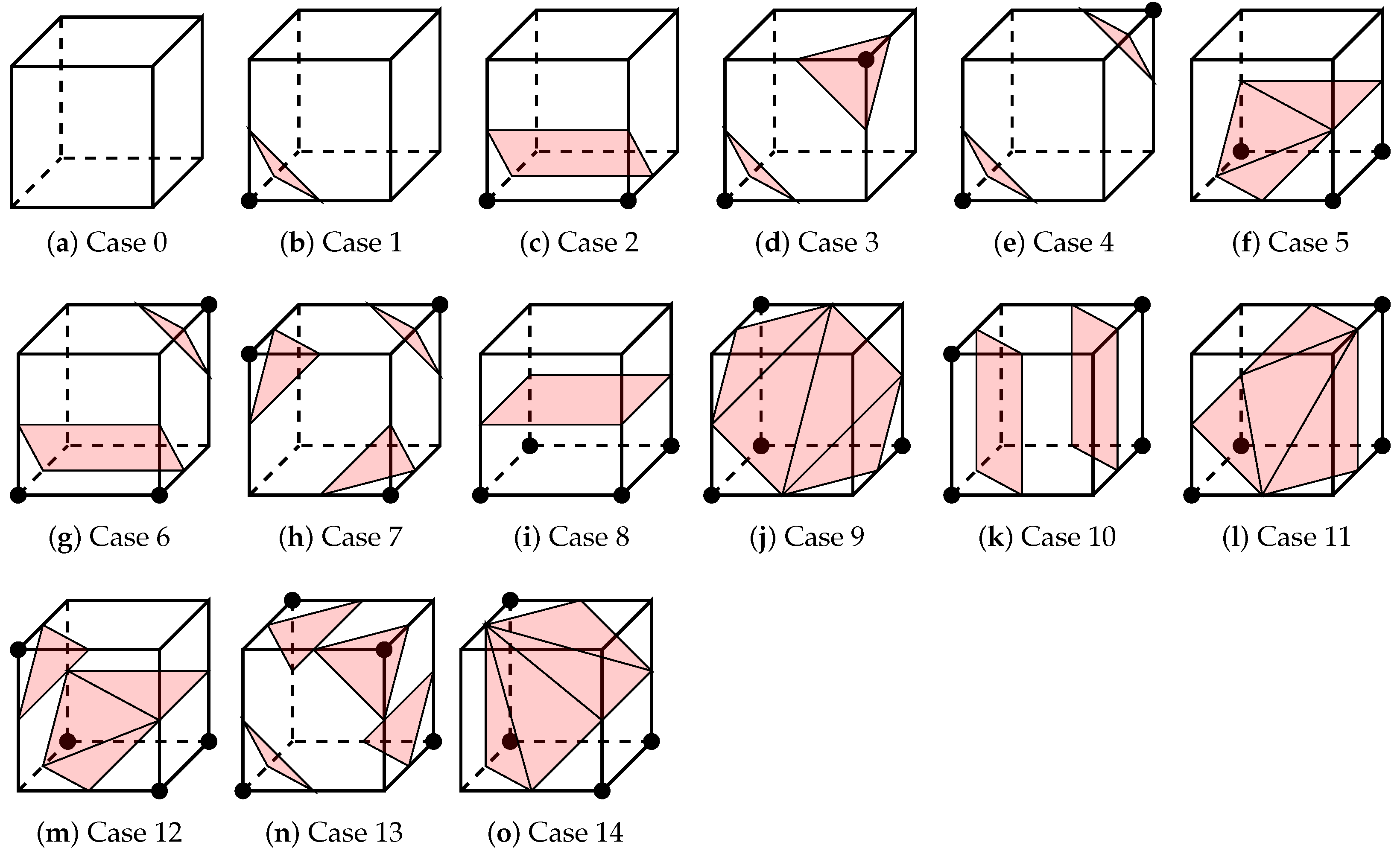
As a marching cube consists of eight vertices, each with two possible states, there are a total of $2^8=256$ different cases. However, only 15 cases are unique, while the remaining cases are simply a combination of inverted, rotated, or flipped variations of the unique instances. The 15 unique variations of a 3D marching cube are depicted in Figure 10 [14].

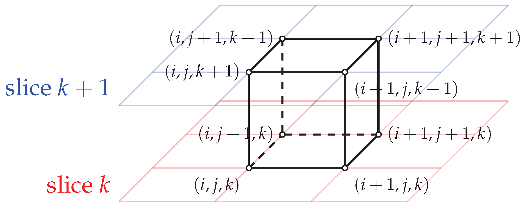
By generating a 3D array of marching cubes in the vicinity of the excavation area as shown in Figure 11, it becomes possible to convert the soil surface into a soil volume. The volume of each marching cube can be pre-calculated, as there is only a finite number of cases. The volume for each case is defined in

Table 1. Volume of the unique cases of marching cubes.

Case No.	Volume	Case No.	Volume	Case No.	Volume
Case 0	0.0000	Case 5	0.3542	Case 10	0.2500
Case 1	0.0208	Case 6	0.1458	Case 11	0.5000
Case 2	0.1250	Case 7	0.0625	Case 12	0.3750
Case 3	0.0417	Case 8	0.5000	Case 13	0.0833
Case 4	0.0417	Case 9	0.5000	Case 14	0.5000

. It is worth noting that in case of inverted variation, the weight would be complement of the given values in Table 1. Summing up the volumes of all the marching cubes enables estimation of the total soil volume within the excavation area. By multiplying the volume by the density of the soil, it is possible to estimate the total weight of the soil as well.

The results obtained from this method are reliable, deterministic, and computationally efficient, ensuring accurate reconstruction and volume estimation for excavation planning.

4. Implementation

A key criterion for selecting approaches for the proposed algorithm is ensuring computational feasibility for real-time implementation. To this end, the authors aimed to design algorithms that leverage parallel computation extensively, achieving significant performance improvement by utilizing GPU computations wherever possible, rather than relying solely on the CPU.

For the curve approximation, each row of the depth image is approximated independently of the others. This characteristic allows the depth image to be divided into hundreds or even thousands of parallel computations, depending on its size. These computations can be assigned to the same GPU simultaneously, enabling efficient processing.

Similarly, the marching cubes algorithm can evaluate and estimate cubes as separate entities, making it highly suitable for parallel computation on a GPU. This approach significantly accelerates the process compared to sequential CPU-based implementations.

To implement the developed algorithm, the authors combined efficient C++ code with CUDA, taking full advantage of the GPU’s parallel processing capabilities.

Figure 12 represents the overall flowchart of the developed algorithm, and the hardware assigned for each task. It is shown that the majority of the computation is done on GPU alone and CPU is only used for transmitting data back and forth from system and GPU memory while needed. In this study, A laptop from Lambda, based in San Francisco, US, featuring an Intel Core i7-8750H processor, 32 GB of DDR4 RAM, and an Nvidia GeForce RTX 2070 Max-Q GPU was used to perform the implemented algorithm.

5. Results and Discussion

This section describes the experiments conducted to validate the performance, accuracy, and efficiency of the proposed algorithm, as outlined in Section 4.

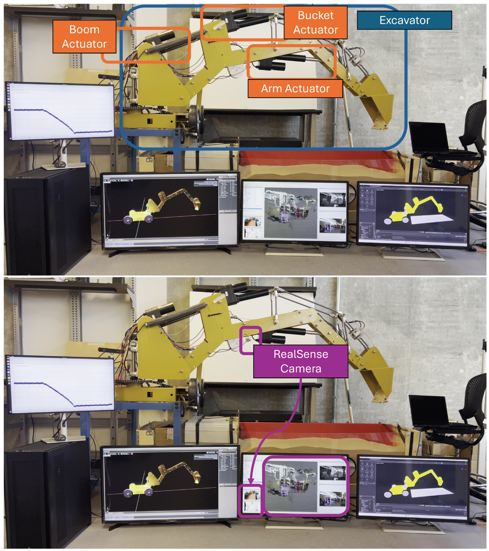
The experiments were performed on an electric excavator, as shown in Figure 13. The depth camera was mounted on the excavator’s boom link to provide an unobstructed view of the excavation area. The camera used in this experiment was the Intel^® RealSense™ Depth Camera D455 from US.

The experimental procedure involved capturing a depth image of the soil surface. The excavator then performed a single digging cycle, and the excavated soil collected in the bucket was weighed to obtain ground truth data. This procedure was repeated twice consecutively.

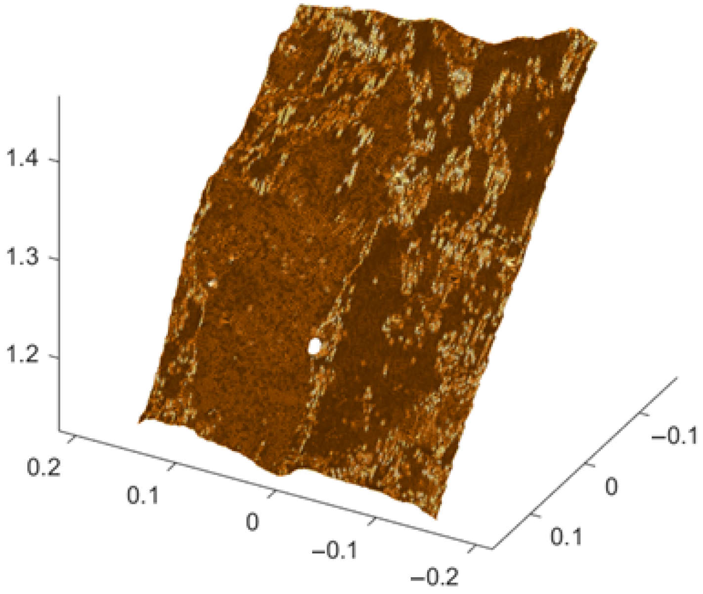
To validate the accuracy of the curve approximation, the raw data points and the approximated curves were plotted to visualize the results of the developed surface reconstruction algorithm. This validation performed before the first digging cycle, after the first digging cycle, and after the second digging cycle. The results for all three datasets are presented in Figure 14.

As illustrated in Figure 14, the reconstructed surface smooths out outliers and provides an accurate mathematical representation based on Equations (5) and (11) for the soil surface.

In order to compare the proposed method with traditional approaches, the same data is used with the Poisson surface reconstruction. This method generates a 3D surface from a point cloud and the normal vector at each point by solving a Poisson equation. It estimates a scalar field whose divergence matches the input normal field. If normals are not provided, they must be estimated, typically using local surface approximations or principal component analysis, which further increase the computation time. The results are shown in Figure 15.

One critical drawback of the traditional approaches is the lack of guarantee that the resulting surface is hole-free. The Poisson method fails to maintain the continuity of the soul surface resulting in a hole as shown in Figure 16.

In addition to the Poisson method, the Crust algorithm also suffers from critical limitations in hole-filling. Although it is designed to reconstruct surfaces from unorganized point clouds, it fails to robustly recover topological consistency in regions with sparse sampling or complex geometry. This often results in incomplete reconstructions with visible holes, as highlighted in Figure 17.

In addition, the Poisson method and Crust algorithm are more resource intensive. The computation time for the proposed approach, Poisson method, and Crust algorithm is presented in

Table 2. Surface reconstruction computation time.

Data No.	Proposed	Poisson	Crust
Data 1	0.08 s	25.27 s	3.2 s
Data 2	0.08 s	25.24 s	3.3 s
Data 3	0.07 s	24.72 s	3.2 s

.

Subsequently, marching cubes models were generated for each of the three datasets based on their corresponding reconstructed surfaces. The soil volumes were calculated at each step. By subtracting the volumes before and after each digging cycle, the volume of removed soil was estimated. Multiplying the estimated volume by the soil density yields the equivalent mass of the excavated soil. These results were compared with the measured weight of the soil collected during the tests and presented in

Table 3. Estimated and actual mass, relative error, and computation time of excavated soil.

Digging No.	Estimated Mass	Actual Mass	Relative Error	Marching Cubes Computation Time
Cycle 1	2.752 (kg)	2.888 (kg)	%4.92	0.05 (s)
Cycle 2	4.791 (kg)	4.723 (kg)	%1.42	0.05 (s)

.

To evaluate the accuracy of surface reconstruction, the raw point cloud generated by the depth camera was compared against the reconstructed surface produced by the proposed method. Additionally, the same raw point cloud was processed using the Poisson method, and the results were compared to assess relative performance.

Finally, to validate the accuracy of the marching cubes method, the soil volume before and after digging was estimated using the marching cubes approach. The difference between these volumes was expected to match the amount of soil collected by the bucket during the excavation.

6. Conclusions

This paper proposes a fast, efficient, accurate, and flexible approach to convert the noisy sensory depth image information of the soil into a surface and volume representation. It is shown that the proposed method is less computationally heavy in comparison with conventional methods by more than 300 times. Also, it provides an efficient method to calculate the metrics such as surface area, volume, and mass of the soil which are important metrics in the earth moving applications. The proposed method efficiently reconstructs surfaces by leveraging connectivity data from neighboring points in the depth image, eliminating the need for additional optimization. Furthermore, it extensively utilizes parallel computation during the curve approximation and marching cubes to further enhance performance.

In addition, the nature of the proposed algorithm can make benefit of parallel computations by accelerating the computational speed by using a GPU. The low computation time also make the proposed algorithm suitable for simulation and machine learning applications.