1. Introduction
In recent decades, the urgency of the climate change-induced increase in the frequency and severity of extreme weather events, particularly floods, has become increasingly evident. The IPCC Sixth Assessment Report (AR6) confirms with high confidence that anthropogenic climate change has already intensified heavy precipitation events in many regions, thereby elevating the risk of both pluvial and fluvial flooding [IPCC, 2021] [
1]. This is further corroborated by recent studies such as that by Lakshmi, V. [
2] which analyzed the Eastern Shore in Virginia using CMIP6-based projections and found a significant increase in flood frequency and severity; an up to 8.9% higher peak flood intensity compared to the 2003–2020 baseline. Their findings also underscore the growing vulnerability of low-lying coastal areas to sea-level rise and hydroclimatic extremes, reinforcing the need for adaptive planning and risk mitigation strategies.
These events pose significant threats to community safety and environmental sustainability, causing substantial damage to infrastructure, ecosystems, and human lives [
3]. This urgency underscores the need to develop practical predictive tools for risk management. Numerous studies, including those from the IPCC, have demonstrated that the intensification of natural disasters, especially floods, is closely linked to human activities [
1]. Uncontrolled urbanization, deforestation, soil sealing, and greenhouse gas emissions all contribute to alterations in the natural hydrological cycle, increasing the frequency and severity of extreme events. The Climate Change 2021 report investigates this relationship’s scientific and physical basis, thoroughly addressing short-term climate forcings in the atmosphere [
4]. This interaction between natural factors and anthropogenic pressures makes flood risk forecasting a complex but essential challenge for enhancing territorial resilience.
In Italy, recent events, including the floods in Emilia-Romagna and an increase in intense weather phenomena in 2024, have underscored the region’s vulnerability. Floods, one of the most common natural disasters, are driven by various factors: heavy rainfall, rising sea levels, inadequate drainage systems, and increasing urban development. The consequences can be devastating, impacting human lives, infrastructure, the economy, and the environment.
To address these issues, both the European Union and Italy have implemented regulatory measures such as Flood Risk Management Plans (FRMPs) [
5] and the Hydrogeological Asset Plan (PAI). These tools aim to prevent and mitigate hydrogeological risks through integrated and up-to-date planning.
Scientific research has produced numerous forecasting models for risk areas. Traditional hydrological models, such as deterministic models based on physical equations, have been extensively used to simulate how watersheds respond to meteorological events [
6,
7]. However, these models require a detailed understanding of the territorial characteristics and often struggle to adapt to complex and dynamic scenarios.
To address these limitations, numerical and probabilistic models have been increasingly adopted. Numerical models, like HEC-RAS, TUFLOW, and OpenFOAM, enable one-dimensional, two-dimensional, or three-dimensional simulations of water flow, offering a more realistic depiction of water propagation [
8,
9,
10]. On the other hand, probabilistic models, such as Bayesian networks and the Analytic Hierarchy Process (AHP), facilitate the quantification of uncertainty while integrating multiple criteria into risk assessments [
11,
12,
13].
Concurrently, artificial intelligence (AI) has introduced transformative methodologies in environmental modeling, particularly in the domain of flood risk assessment. Machine learning (ML) algorithms such as Random Forest (RF), Support Vector Machines (SVMs), and deep neural networks have demonstrated strong capabilities in processing large-scale, heterogeneous environmental datasets, including meteorological time series, topographic features, land use classifications, and hydrological indicators. These models are particularly effective in capturing complex, nonlinear interactions among variables, enabling the classification of flood-prone areas and the forecasting of extreme events with enhanced accuracy. For instance, RF is widely adopted for its robustness, interpretability, and suitability for spatial risk mapping, while deep learning architectures such as Long Short-Term Memory (LSTM) networks and Convolutional Neural Networks (CNNs) are increasingly employed to model temporal dependencies and spatial patterns in flood dynamics. These AI-driven approaches are reshaping predictive modeling in environmental sciences by offering scalable, data-driven solutions that complement or surpass traditional hydrological models [
14,
15,
16,
17,
18].
Additionally, the integration of sequential models, such as Long Short-Term Memory (LSTM) [
19], has enhanced temporal event prediction by capturing long-term dependencies in historical data. However, these models require significant computational resources and a complex training phase.
In this context, flood risk forecasting is crucial in spatial planning and civil protection. However, the current state of traditional forecasting models that rely on hydrological or statistical approaches is not without its limitations. These models often struggle with accuracy and adaptability to complex and dynamic scenarios, highlighting the need for a new approach.
This study proposes an innovative approach that could potentially revolutionize flood risk forecasting. It integrates machine learning algorithms, specifically Random Forest, with Markov chains. It utilizes high-resolution data derived from LIDAR, lithological maps, land use, and precipitation to improve the accuracy of flood risk assessments and support informed decision-making in land management.
The main contributions of this work include the following:
Developing a hybrid RF–Markov predictive model for the dynamic simulation of flood risk.
The use of LIDAR data to generate high-resolution digital terrain models.
A quantitative comparison with LSTM models to validate the effectiveness of the proposed method.
Creating flood susceptibility maps to aid urban planning and mitigation strategies.
The recent literature has explored employing deep learning techniques and probabilistic models for flood prediction. However, the effective integration of spatial accuracy and temporal modeling is often lacking. Our approach bridges this gap by combining the robustness of tree-based models with the capability of Markov chains to model the temporal evolution of risk.
Our challenge is the difficulty of accurately predicting flood-prone areas in complex urban environments. Our model addresses this issue by integrating geospatial and temporal data into a predictive framework that is interpretable, efficient, and adaptable to various territorial contexts.
3. Materials and Methods
In recent years, the increasing frequency and intensity of floods have highlighted the urgent need for more effective forecasting models. Research on flood monitoring and mapping has expanded, not to directly mitigate the impacts of land and urban changes, but rather to provide essential support for informed decision-making and targeted actions to address these challenges. Models have evolved over the past three decades. Time series models (TSMs) were dominant in flood prediction until 2010, while machine learning (ML) models, especially artificial neural networks (ANNs), have been the most dominant since 2011. Despite significant advancements, there remains potential for further integration of machine learning algorithms with other techniques to enhance predictive accuracy.
This study contributes to this effort by introducing an innovative approach that combines Random Forest with Markov chains, leveraging LIDAR data and geospatial information to enhance flood risk prediction. Developed in Python 3.11.2, this model delivers high spatial accuracy, which is crucial for identifying vulnerable areas and guiding proactive interventions. Rather than acting as a direct solution to flood-related challenges, this system serves as a valuable resource for local authorities, empowering them to make informed land management and urban planning decisions to mitigate risks effectively.
Figure 1 presents a graphical representation of the phases and data involved in flood risk assessment. Each process step, from data collection to modeling and validation, is outlined to emphasize the integrated and multidisciplinary approach adopted. This methodology considers various topographical and environmental factors influencing flooding, ensuring a more accurate and reliable risk assessment. The outcome of this process is the flood susceptibility map (FSM), which serves as a crucial tool for spatial flood risk assessment. It aids in identifying areas at risk and facilitates the planning of mitigation measures
. The Random Forest model was chosen for its proven accuracy and robustness compared to other machine learning algorithms [
29,
30]. While more advanced models, such as deep neural networks, exist, Random Forest strikes an optimal balance between interpretability, training speed, and predictive performance. This makes it particularly suitable for applications requiring a clear understanding of model decisions. Additionally, its lower susceptibility to overfitting enhances its reliability, making it a preferred choice for predictive analytics in complex environments.
The integration of advanced technologies, such as machine learning and Markov chains, facilitates the identification of high-risk areas and supports more informed land management decisions. These tools enable the analysis of large volumes of historical and current data, helping to identify patterns and trends that contribute to more accurate flood forecasting. Ultimately, this approach aids in disaster mitigation and community protection.
The Random Forest model introduces an element of randomness in selecting features for each tree, which helps reduce the correlation between trees and enhances the overall robustness of the model (
Figure 2).
The process can be broken down into the following phases:
Generating Subsets of Features: A random subset of features is selected from the original dataset for each node in a tree. This subset is much smaller than the available features, ensuring tree diversity.
Determining the Optimal Feature: Among the randomly selected features, the one that best optimizes data separation is identified using quality metrics such as entropy or the Gini index.
Iterating the Process: This process is repeated for every node in every tree, ensuring that each tree is constructed using a unique set of features. This ensemble approach enhances the model’s ability to generalize to unseen data.
Before starting the model training, it is essential to configure several key hyperparameters.
A hyperparameter search technique should be applied to determine the parameters that optimize the model’s predictive performance. The proposed study selected Grid Search for its comprehensiveness, simplicity, and reliability.
The specific hyperparameter considered in this study was:
- -
n_estimators: This refers to the number of trees in the forest. A higher number of trees enhances the model’s performance by reducing variance.
- -
max_features: This parameter specifies the number of features to consider when splitting each node. By using ‘sqrt,’ you ensure that each tree is trained on a distinct subset of characteristics, which enhances diversity and minimizes the risk of overfitting.
- -
max_depth: This defines the maximum depth of each tree. A greater depth allows for the capture of more complex patterns, but intense trees can lead to overfitting. It is important to find a balance when selecting the depth.
- -
min_samples_leaf: This parameter sets the minimum number of samples required to form a leaf. It helps prevent the creation of overly specific subdivisions that may contribute to overfitting.
- -
min_samples_split: This indicates the minimum number of samples to split a node. Similarly to min_samples_leaf, this parameter aims to reduce excessive subdivisions.
The rationale for choosing these hyperparameters is based on achieving a balance between model accuracy and computational efficiency. Increasing the number of trees (n_estimators) improves model performance by reducing variance, but too many trees can increase computation time without significant performance gains.
A value of 300 was chosen as a good compromise between accuracy and computational efficiency. The limitation in its choice is dictated by computational constraints and the need to contain training times.
Setting max_features to ‘sqrt’ ensures that each tree is trained on a different subset of features, increasing diversity among the trees and reducing their correlation. This enhances the model’s robustness.
Selecting a max_depth of 30 enables the model to capture complex patterns while preventing overfitting. Min_samples_leaf and min_samples_split help prevent overly specific subdivisions, improving the model’s generalization.
The hyperparameter search was conducted using Grid Search, which explores all possible combinations of a predefined set of hyperparameters (
Table 1). This technique ensures that no potentially optimal combination is overlooked. The study used the fit method to train the model on different combinations of hyperparameters as part of the Grid Search process. This method is crucial because it enables the model to learn from the data and adjust its internal parameters to minimize prediction error.
Cross-validation was used to evaluate the model’s performance on different sections of the dataset. A 3-fold cross-validation was employed, dividing the dataset into three parts and training and validating the model three times for each combination of hyperparameters. The dataset consisted of spatial units (grid cells) characterized by environmental and topographic features: elevation, land use, lithology, and average rainfall. These features were extracted from LIDAR, CORINE Land Cover, and ARPACAL rainfall data (2014–2024). The target variable (predictand) was the flood risk class assigned to each unit, categorized into four ordinal levels (low, moderate, high, very high), derived from PCA-based classification. The expression “different sections” refers to the three subsets created during 3-fold cross-validation. The dataset was randomly partitioned into three equal parts. In each iteration, two-thirds were used for training and one-third for validation, rotating the folds across three runs.
After completing the Grid Search, the best-performing model is selected based on the chosen evaluation metric, which in this case was accuracy, equal to 0.87 during the hyperparameter optimization phase. This value represents the proportion of correctly predicted flood risk classes across the validation folds and was used exclusively to guide the selection of the optimal parameter combination during Grid Search. The optimal parameters identified were n_estimators = 300, max_depth = 30, min_samples_split = 2, min_samples_leaf = 1 and max_features = ‘sqrt’ (
Table 2). The total number of hyperparameter combinations is calculated as the product of the number of candidate values for each parameter:
n_estimators: 3 values ([100, 200, 300])
max_depth: 4 values ([None, 10, 20, 30])
min_samples_split: 3 values ([2, 5, 10])
min_samples_leaf: 3 values ([1, 2, 4])
max_features: 2 values ([log2, ‘sqrt’])
The total number of combinations would be: 3 × 4 × 3 × 3 × 2 = 216. The parameter ‘sqrt’ in the context of Random Forest refers to the number of features to consider when looking for the best split; ‘sqrt’ indicates that the number of features considered in each split is the square root of the total number of features. This approach balances the diversity of individual trees and the reduction of overall model variance. The log2 parameter indicates that, for each split of a tree, the maximum number of features to consider is the base 2 logarithm of the total number of available features. This value reduces the number of features evaluated at each node, increasing diversity between trees and improving model generalization. These are standard options in the Random Forest implementation in Python and are used to control the number of features considered at each split, balancing model diversity and variance reduction.
To ensure reproducibility, we have made the full dataset structure, preprocessing steps, and model code publicly available at:
http://github.com/Luigi2020357/Flood-Forecast. This includes the scripts used for feature extraction, model training, and evaluation. For further details, please refer to
Appendix A.
Markov chains are widely used for modeling probabilistic systems that evolve over time, providing insights into environmental and anthropogenic interactions [
31]. In flood forecasting, each state represents a different level of risk, transitioning probabilistically based on current conditions rather than past history, an attribute known as the Markov property or “short memory” [
32,
33].
A transition matrix
P is used to describe these transitions mathematically. Each element of the matrix,
Pij, indicates the probability of moving from state
i to state
j in a single step. The transition matrix is defined as follows:
where
Pij is the probability of transition from state
i to state
j. The sum of the probabilities of transition from a state must be equal to 1, i.e.,
In homogeneous Markov chains, (P) remains constant, and the stationary probability distribution π satisfies the equation πP = π, ensuring equilibrium over time.
Conversely, non-homogeneous Markov chains allow for transition probabilities to vary over time or due to external influences [
34]. This adaptability enables the definition of multiple transition matrices (
P_t) for different time intervals, reflecting environmental changes.
An important concept in Markov models is absorbent states, which represent situations in which, once reached, the system remains indefinitely, such as extreme flood risk scenarios.
Markov chains can be classified as regular or ergodic:
- -
Regular chains ensure that any state can be reached within a finite number of steps.
- -
Ergodic chains exhibit stable long-term behavior, converging toward a unique stationary distribution, irrespective of the initial state. For further details, please refer to
Appendix B.
The Long Short-Term Memory (LSTM) model was used as a benchmark comparator to evaluate the predictive performance of RF against a more complex, sequence-oriented deep learning model. Our goal was to compare the following two fundamentally different approaches:
- -
Random Forest: a robust, interpretable, and computationally efficient model, well-suited for heterogeneous environmental data.
- -
LSTM: a deep learning model capable of capturing temporal dependencies, but more computationally intensive and less interpretable.
This comparison enabled us to highlight the strengths and limitations of each model in the context of flood risk prediction. The results showed that RF achieved higher accuracy (0.89 vs. 0.85), better precision and recall, and significantly faster training times, confirming its suitability for the task, especially when interpretability and efficiency are important.
LSTM is a specialized recurrent neural network (RNN) designed to process sequential data while overcoming the limitations of traditional RNNs in capturing long-term dependencies. This capability makes LSTM particularly effective for analyzing time series, such as meteorological and hydrological forecasts.
Its architecture incorporates memory cells that regulate data retention through the following three fundamental components:
- -
Input gate—which updates the cell state with relevant new information.
- -
Forget gate—which discards unnecessary data.
- -
Output gate—which selects the most relevant information for prediction.
By integrating multimodal data sources (e.g., satellite imagery, meteorological records, and hydrological datasets), LSTM enhances predictive accuracy by reducing biases and errors.
Training the model involves Backpropagation Through Time (BPTT), an advanced optimization method that unrolls the network over time, mitigating vanishing and exploding gradients issues common in traditional RNNs.
Despite its effectiveness, LSTM is computationally demanding and requires careful hyperparameter tuning to achieve optimal performance. In this study, the LSTM model was not used with default parameters. Instead, it was systematically optimized using GridSearchCV in combination with TimeSeriesSplit cross-validation. The following hyperparameters were explored:
Batch size: [16, 32, 64].
Epochs: [50, 100].
Optimizers: [‘adam’, ‘rmsprop’].
Dropout rates: [0.2, 0.3, 0.4].
This resulted in a total of 36 combinations, each evaluated using 5-fold time series cross-validation, for a total of 180 training runs. The model was wrapped using KerasRegressor to ensure compatibility with GridSearchCV. The best-performing configuration was selected based on validation loss, and the final model was retrained using the optimal parameters. The training and performance metrics (MSE, RMSE, R2) were computed and visualized accordingly.
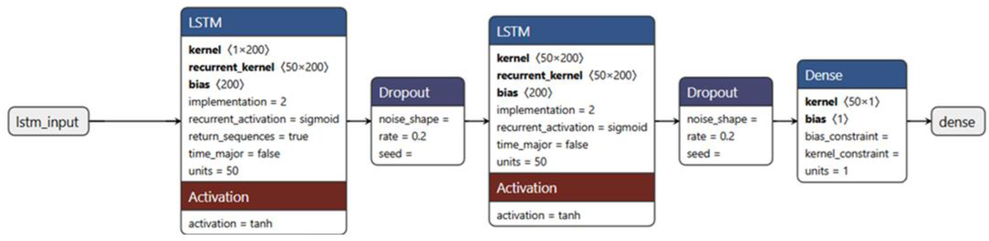
The architecture of the optimized network, illustrated in
Figure 3, includes several layers.
This means that the model takes as input sequences of 60 timesteps, each with a single characteristic.
return_sequences=True: This parameter indicates that the LSTM layer returns the entire output sequence for each timestep input, which is used as input for the next LSTM layer.
This layer helps prevent overfitting by randomly turning off 20% of neurons during training.
return_sequences=False: This parameter indicates that the LSTM layer returns only the last output of the sequence, which is used as input for the final dense layer.
Similarly to the first Dropout layer, it helps prevent overfitting.
This is the output layer that produces a single prediction.
Filling in the Model.
In this study, we utilized LIDAR (Light Detection and Ranging) data.
LIDAR is a high-resolution remote sensing technology used to model flood-prone areas with remarkable precision [
35]. It employs an IMU (Inertial Measurement Unit) platform, emitting laser pulses to measure distances between the sensor and ground objects, enabling three-dimensional georeferencing.
By scanning terrain, LIDAR generates a point cloud, distinguishing digital terrain models (DTMs) from digital surface models (DSMs). This data allows for precise elevation mapping, with a detection density exceeding 1.5 points/m2 and an altimetric accuracy within 15 cm.
LIDAR-derived digital elevation models (DEMs) play a critical role in hydraulic modeling, particularly in urban environments where high-resolution topography is necessary for assessing flood susceptibility. DEM resolution directly impacts flood propagation accuracy, with research confirming LIDAR-generated DEMs outperform other models [
36,
37].
This methodology provides a reliable framework for hydrological predictions, aiding in the identification of risk areas and supporting effective land management strategies.
3.1. Integration of RF and Markov Chain Models
The integration of the Random Forest (RF) model with the Markov chain presents a sophisticated and complementary approach to flood risk prediction. The RF model utilizes environmental and topographic data, including information derived from LIDAR, to accurately forecast flood-prone areas. Following this, the Markov chain models the temporal evolution of flood risk, simulating the transitions between different hazard levels (low, moderate, high, and very high).
This combination offers a dynamic perspective on risk. The transition matrix, constructed from the RF model’s predictions, quantifies the probabilities of transition between risk states, providing a probabilistic outlook on the future progression of flood risks. The unit of time used for observing transitions between flood risk states is monthly. The dataset spans 11 years, and each year is divided into 12 monthly intervals resulting in a total of 132 time steps. Each time step corresponds to a monthly observation of flood risk classification (low, moderate, high, and very high); an “observation” refers to the monthly flood risk classification assigned to each spatial unit (DEM cell) in the study area. Each unit is characterized by environmental features and receives a predicted risk class at each time step. With 132 time steps (11 years × 12 months), each unit contributes 132 observations to the temporal sequence used in the Markov chain analysis.
In this study, states are used to symbolize different flood risk classes rather than directly representing meteorological or hydrological conditions. These classes are derived from predictions made by the Random Forest model, which incorporates various environmental variables to categorize each spatial unit into one of four distinct risk levels. This method provides a clear understanding of transition processes over time by utilizing a Markov chain to model the evolution of risk. Statistical validation has confirmed the homogeneity of this matrix, indicating that transition probabilities remain stable over time, which reinforces the reliability of the integrated model.
To verify the temporal stability of the transitions between risk classes, we analyzed the homogeneity of the Markov chain by means of G
2 statistics, as proposed by Anderson and Goodman [
38] in their classic treatment of hypothesis testing for Markov chains. In particular, the null hypothesis tested is:
H0:
The transition matrix P describes a homogeneous Markov chain, i.e., the transition probabilities do not vary over time.
To this end, the observation period was divided into two distinct ranges: T1 (2014–2018) and T2 (2019–2024). For each interval a transition matrix (P1 and P2) was calculated, while the aggregate matrix P3, covering the entire period (T1 + T2), was used to estimate the expected frequencies eij below H0.
The
G2 statistic was calculated according to the formula
nij represents the observed frequency of transition from state ii to state jj in periods
T1 and T2;
eij is the expected frequency calculated on the basis of the aggregate matrix P3;
r = c = 4 represents the number of states (risk levels: low, moderate, high, and very high).
The degrees of freedom are equal to (r − 1) × (c − 1) = 9. The G2 test was used to compare the P1 and P2 matrices against the P3 aggregate matrix. The critical value of the chi-square distribution at the significance level of 5% is 16.92. The calculated value of G2 was 2.16, well below the critical threshold, confirming the homogeneity of the Markov chain and the stability of the transition probabilities over time.
This verification reinforces the validity of the integrated RF–Markov predictive model, demonstrating that the observed risk dynamics are statistically consistent over the entire study period.
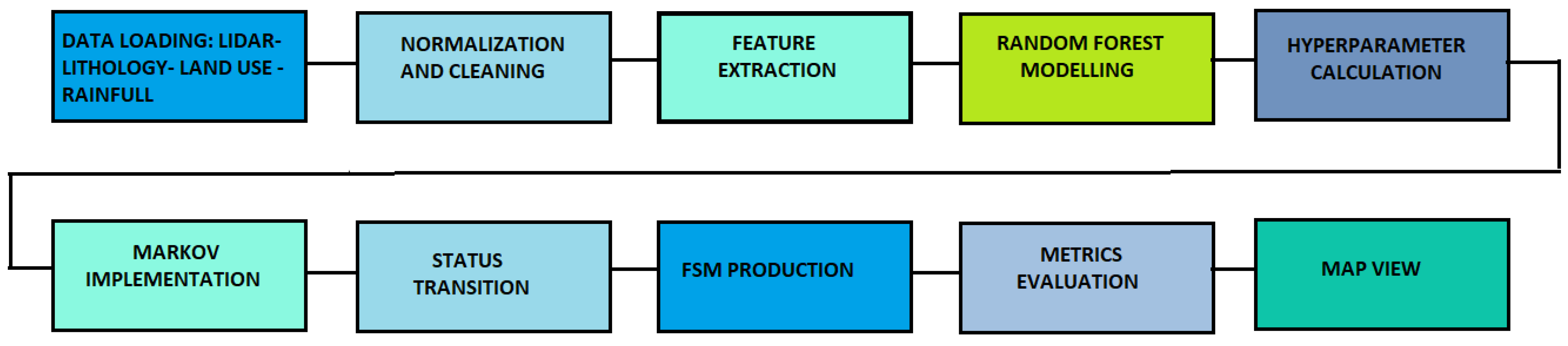
The flood risk forecasting process is structured into several phases, incorporating machine learning techniques, geospatial analysis, and stochastic modeling:
CSV files containing daily rainfall data from the ARPACAL gauge network (Calabria, Italy) were collected for the period 2014–2024. The original data, recorded at hourly intervals, were aggregated to daily totals. Non-numeric values (e.g., sensor errors, missing transmissions) were converted to NaN. Approximately 7.3% of the data were missing, with spatial and temporal variability. Rows with simultaneous NaNs across multiple stations were removed, while isolated gaps were filled using linear temporal interpolation. Stations with excessive missing data were excluded. TIFF files containing elevation data (DEM) are loaded and resized to increase resolution. Land use and lithology maps are loaded and resized to increase resolution. StandardScaler is used, which is a scikit-learn module used to standardize the characteristics of a dataset before being used for model training.
Feature extraction. Feature extraction was performed by combining spatial data on elevation, land use, lithology, and long-term average rainfall. Rainfall data were averaged by first computing the annual mean daily precipitation for each station over the period 2014–2024. These values were then spatially interpolated using ordinary kriging to generate a continuous raster of average rainfall. Each pixel in the study area was assigned the corresponding interpolated rainfall value. All features were then transformed into a structured array for model input. This data is then transformed into an array of features.
To reduce redundancy and improve computational efficiency, Principal Component Analysis (PCA) was applied to the input feature matrix, which included elevation (from LIDAR-derived DEM), land use (from Copernicus CORINE), lithology (from geological maps), and long-term average rainfall (from ARPACAL data). Each raster was spatially aligned and flattened, resulting in a dataset of 84,656 spatial units (pixels), each described by four standardized variables.
PCA was applied globally to the entire feature matrix, rather than separately by feature group, in order to capture the joint variance structure and potential interactions among topographic, geological, and meteorological variables. The transformation was performed after standardization using StandardScaler, ensuring equal contribution from all features regardless of scale.
The number of principal components was determined by setting n_components=0.95, retaining only those components necessary to explain at least 95% of the total variance. This resulted in the retention of seven principal components. The first three components alone accounted for approximately 95% of the variance, with PC1 dominated by lithological variables (especially clay and sandstone), PC2 by limestone, and PC3 by land use classes (notably forest and urban areas).
The Parallel function of joblib is applied to perform operations in parallel, leveraging multiple processors or threads to improve performance and reduce execution time.
Creating the machine learning model. A Random Forest model is trained on training data (80%) to classify areas into different risk classes.
Implementation of the Markov model. A Markov chain is created to predict transitions between risk classes.
Flood risk classification.
Creation of the flood susceptibility map. The model’s forecasts are used to generate a flood risk map, with different risk classes (Low, Moderate, High, Very High).
Maps view. The map is displayed using a color map to highlight the different risk classes.
Figure 4 illustrates the development phases of the RF–Markov model.
Predicting the evolution of flood risk over time is crucial for emergency management and resource allocation. The integrated model provides valuable insights for developing effective mitigation and response strategies, supporting decision-making to protect communities and minimize impacts. Understanding flood timing and progression enhances resource management during emergencies, improving early warning systems and information accuracy. Long-term forecasts aid in creating effective flood risk management plans, including preventive measures like flood barriers and advanced drainage systems.
3.2. Dataset
The flood risk forecasting model is based on four main categories of data: geospatial, environmental, meteorological, and LIDAR, offering an integrated view of the territory.
- -
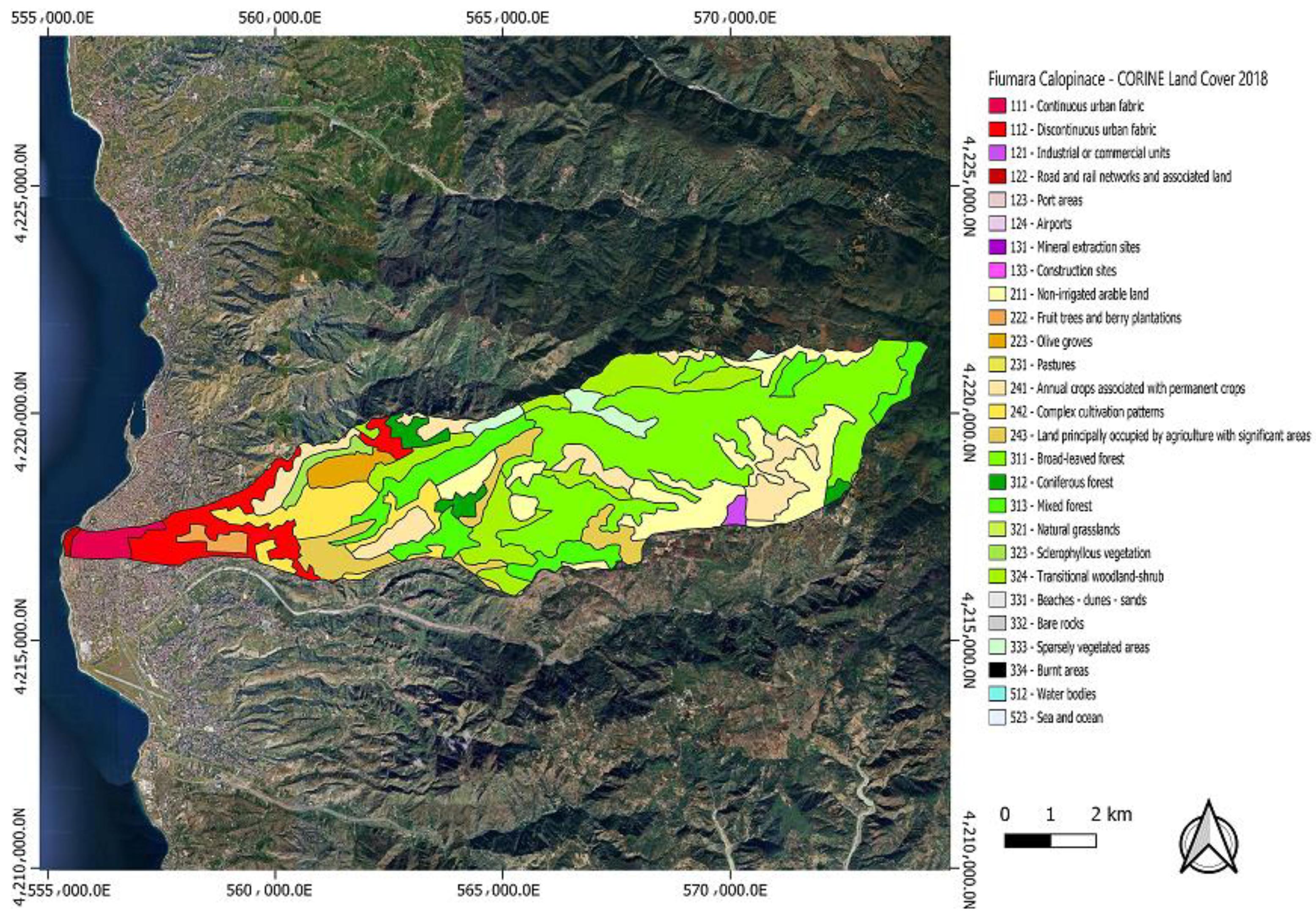
Geospatial Data and Land Use: The geological information comes from the Geological Map of Italy, with a focus on the Calabria Region, to assess soil permeability.
- -
Land use data comes from the CORINE Land Cover project, with a geometric accuracy of 25 m, and is critical for estimating the impact of urbanization on surface runoff. (LIDAR).
- -
Elevation and slope data are obtained from digital elevation models (DEMs) derived from LIDAR surveys, provided by the MASE Extraordinary Remote Sensing Plan (PST). With an elevation accuracy of less than 15 cm, this data makes it possible to identify depressed areas, slopes and water storage areas.
- -
Meteorological Data: Based on eleven years of observations, the rainfall data were obtained from ARPACAL (Agenzia Regionale per la Protezione dell’Ambiente della Calabria), which operates a network of ground-based rain gauges across the region. The spatial distribution of stations is denser in coastal and urban areas, with sparser coverage in mountainous zones. Data were accessed via formal request and processed in compliance with ARPACAL’s data usage guidelines. Limitations include spatial gaps and occasional sensor outages, which were addressed through data cleaning and interpolation strategies as described above.
The integration of meteorological, geological, LIDAR, and land use data was carried out through a methodological approach that leverages the distinct characteristics of each dataset. Meteorological data, collected daily over 11 years, represent the dynamic component of the model, capturing rainfall variability, one of the main drivers of flood events. This variability is modeled using Markov chains to simulate transitions between different risk states over time. In contrast, geological and LIDAR data provide a high-resolution, static representation of the territory’s physical and morphological features, such as lithology, elevation, and slope. These datasets are fundamental for defining the intrinsic susceptibility of the territory to water accumulation and outflow. Land use data, while spatially detailed, are not strictly static. Changes in land cover due to urban expansion, deforestation, or agricultural transformation can significantly alter surface runoff and infiltration capacity over time. Therefore, land use is treated as a semi-dynamic variable, whose influence is modeled in combination with meteorological variability.
The integration of these datasets occurs within the Random Forest model, which combines spatial information (e.g., lithology, elevation, land use) with dynamic meteorological data (precipitation) to classify areas into different flood risk categories. While lithology and elevation remain constant over the 11-year simulation period, land use and rainfall introduce variability—rainfall through monthly time series, and land use through its spatial heterogeneity and potential for change.
This temporal component is further modeled using a Markov chain, which simulates the probabilistic evolution of flood risk over time based on the initial classifications provided by the Random Forest model.
In summary, static data define the spatial predisposition to risk, while rainfall and land use dynamics drive temporal and spatial variability. This synergy enables the model to capture both structural and evolving aspects of flood risk, enhancing strategic understanding and forecasting capabilities.
The results of the application of this methodology, presented in the following section, demonstrate the model’s effectiveness and accuracy in identifying high-risk areas.
5. Results
The data used in our study consisted of rainfall data collected by ARPACAL over the past eleven years, from 2014 to 2024, lithological and land use data. Additionally, the LIDAR data relevant to the study area were sourced from the PST (Extraordinary Remote Sensing Plan) database [
39]. This database, provided by the Ministry of the Environment and Energy Security (MASE), contains geospatial and earth observation information that can be utilized to monitor and predict environmental and territorial phenomena.
Although there is no specific and universally recognized standard for selecting causal factors of floods that influence flood events [
40], the interaction between various topographical and environmental factors plays a crucial role in flood risk assessment. The following factors were taken into account in the study:
Rainfall Data: This provides the amount, intensity, and duration of rainfall. Heavy, prolonged rainfall can saturate soils and increase surface runoff, thereby heightening flood risk.
Land Use: Urbanized areas with impermeable surfaces (e.g., roads, buildings) reduce water infiltration, while regions with natural vegetation absorb more water, lowering flood risk.
Lithology Map: The composition and structure of subsurface rocks and sediments affect water absorption. Porous materials like sand absorb more water than compact ones like clay, influencing runoff behavior.
LIDAR Data and DEMs: High-precision LIDAR data supplies detailed topographic information (elevation and slope) crucial for modeling water flow. Digital Elevation Models (DEMs) derived from LIDAR data help predict water accumulation and identify flood-prone areas. Two types of models are commonly used:
DSMFirst: Captures the first return of the laser, including buildings, trees, and other surface objects.
DSMLast: Captures the last return, focusing on the bare ground to produce a more accurate terrain representation. By removing surface features, a precise Digital Terrain Model (DTM) is obtained.
These data are integrated to simulate floods: LIDAR files are loaded to create the DEM, features are extracted, and all the information feeds into the Random Forest–Markov chain forecasting model. This model analyzes the combined topographical and environmental factors to assess flood risk accurately.
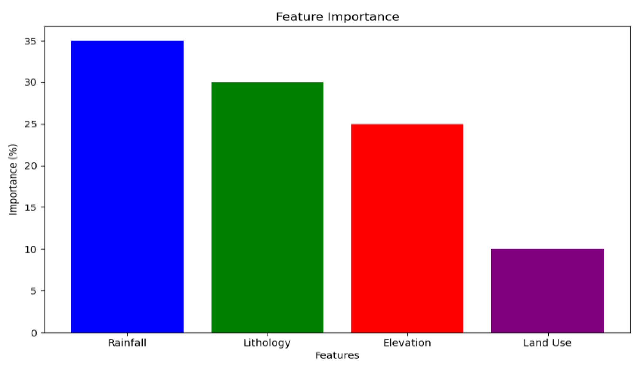
The feature importance values shown in
Figure 8 are derived from the Random Forest model and are expressed as percentages. These values represent the relative contribution of each feature to the model’s predictive performance, typically calculated using the mean decrease in impurity (Gini importance) across all decision trees in the ensemble. In this case, rainfall contributes approximately 35%, lithology 30%, elevation 25%, and land use 10% to the classification of flood risk.
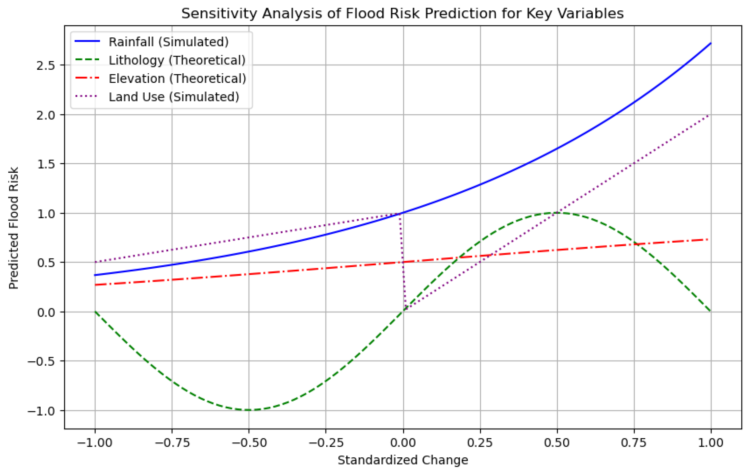
Along with feature importance plots, a sensitivity analysis was performed to assess how changes in input variables affect model predictions. The results of this analysis are illustrated in
Figure 9, which displays the model’s response to changes in key variables.
While lithology and elevation are static variables, both rainfall and land use can vary over time and space. In particular, land use changes due to urbanization, deforestation, or agricultural practices can significantly alter surface runoff and infiltration capacity.
Figure 9 reflects this distinction by showing simulated sensitivity curves for rainfall and land use, and theoretical curves for lithology and elevation. This approach enables us to capture both the dynamic and structural components of flood risk, providing a more realistic and comprehensive understanding of how each factor contributes to flood hazard.
Sensitivity analysis is essential for understanding and managing flood risk.
The figure illustrates how standardized changes in four key variables, Rainfall, Land Use, Lithology, and Elevation, affect predicted flood risk. Rainfall (solid blue line) and Land Use (dotted purple line) are treated as dynamic variables, with curves derived from model-based simulations. Lithology (dashed green line) and Elevation (red dash–dot line) are considered static variables, and their curves represent theoretical relationships based on hydrological reasoning and their contribution to the model’s classification. All curves are plotted on a uniform y-axis scale to enable the direct comparison of their influence on flood risk.
These variables interact complexly, making an integrated analysis of all the essential factors in flood risk assessment. The assignment of weights to environmental factors in our model was determined through a sensitivity analysis, which identified the variables with the greatest impact on flood susceptibility. Rather than directly applying these weights, we employed Principal Component Analysis (PCA) to synthesize the information from the most influential variables into a reduced set of uncorrelated components. PCA allows for dimensionality reduction by eliminating redundancies and generating principal components that represent optimal linear combinations of the original variables.
To classify flood susceptibility levels, we employed a synthetic index derived from the first principal component (PC1) of the PCA. The classification into four susceptibility classes (Low, Moderate, High, and Very High) was based on quartile thresholds of the PC1 scores. This statistical approach was adopted to ensure objectivity and comparability across spatial units in the absence of consistent hydrological benchmarks or flood incidence records. Importantly, this classification was used solely for spatial interpretation and visualization purposes, and not as a target variable in model training.
PCA loadings were carefully interpreted to retain physical meaning, and a sensitivity analysis was conducted to assess the influence of individual variables (see
Figure 9). The resulting susceptibility map represents a relative environmental predisposition to flooding, not an absolute hazard measure. Limitations of this approach are acknowledged, and future work will focus on calibrating the classification using hydrodynamic models, historical flood data, and, where feasible, ground-truthing.
This approach makes it possible to identify the most vulnerable areas with objective criteria, avoiding distortions resulting from an arbitrary choice of classification parameters.
Through this strategy, the model is able to integrate the relative importance of features with a robust aggregation method, improving the accuracy of flood risk prediction and facilitating the interpretation of results.
The risk classes identified are as follows:
Low: R < T1;
Moderate: T1≤R<T2;
High: T2≤R<T3;
Very High: R≥T3.
Risk class thresholds (quartile-based)
Class|Risk index range
Low| ≤ −0.34
Moderate|−0.34 to 0.01
High|from 0.01 to 0.34
Very High| > 0.34
Negative values indicate environmental conditions that are less favorable to flooding than average. Positive values indicate more risk-prone conditions.
The classification into quartiles does not imply that 50% of the territory is at absolute risk, but that in relation to the sample, half of the areas have more favorable conditions for flooding.
The classification of flood susceptibility was performed independently from the model training phase. A synthetic index was computed for each area using a weighted combination of environmental variables (rainfall, lithology, land use, and altitude), based on their relative importance. This index was then divided into quartiles to identify areas with different levels of susceptibility: Low, Moderate, High, and Very High.
This classification was not used as a target variable for model training. The Random Forest model was trained separately using 80% of the dataset, with meteorological data and environmental variables.
The quartile-based classification serves as a complementary tool for spatial interpretation, allowing for the identification of areas with similar environmental conditions that are more or less favorable to water accumulation and runoff. This approach ensures objectivity and reproducibility in the absence of historical flood records, and is grounded in real, observed data.
The predictions of the model are used to construct the transition matrix.
Figure 10 presents the transition probability matrix derived from the full time series of historical flood risk classifications. The matrix captures the stochastic dynamics of flood risk evolution across all available monthly observations. Each cell represents the normalized probability of transitioning from one risk state to another (Low, Moderate, High, Very High) based on observed transitions over time. This matrix is spatially aggregated and reflects the average behavior across the entire study area.
The transition matrix is a square matrix in which each element (i, j) represents the number of transitions observed from state i to state j in the model’s predictions.
The predictions generated with the Markov chain are obtained starting from the initial state (first prediction of the model) and for each subsequent step, the transition matrix is used to determine the probability of transition to the subsequent states. The next state is chosen based on the probability of transition. The transition matrix obtained represents the probabilities of transition between different states of flood risk: low, moderate, high, and very high. Numeric values are displayed within cells for clarity. The values are represented with different colors to identify the level of risk.
Analyzing the data reveals that low-risk areas have a 22.2% chance of remaining in their current state. However, they also have a 22.2% probability of transitioning to a moderate-risk state. Additionally, there is a slightly higher probability of 27.8% that these areas will move to a high or very high-risk state.
Moderate-risk areas have a 10.7% chance of improving and moving to a low-risk state. They also have a 28.6% probability of remaining in the moderate-risk category. However, the likelihood of worsening and transitioning to a high-risk state is 35.70%, and 24.0% for escalating to a very high-risk state.
It is important to note that while the probability of worsening from moderate to high is significant, the reverse transition, from high to moderate, has an even higher likelihood (46.4%). This suggests that high-risk areas are statistically more likely to improve than moderate-risk areas are to deteriorate, highlighting the dynamic and potentially reversible nature of flood risk in certain zones.
High-risk areas show a 14.3% chance of improving and transitioning to a low-risk state. They have a significant 46.4% probability of moving to a moderate-risk state. The probability of staying in the high-risk category is relatively low, at 17.9%, while there is a notable 22% chance of moving to a very high-risk state.
Lastly, areas categorized as very high-risk have a 28.0% chance of improving and transitioning to a low-risk state and a 16.0% chance of moving to a moderate-risk state. The probability of moving to a high-risk state or remaining in the very high-risk category is 32.0% and 24.0%, respectively.
For instance, the probability that a moderate-risk area may escalate to a high-risk state (35.7%) indicates the need for prioritized monitoring and preventive measures. Thus, the transition matrix serves not only as a descriptive tool but also as a valuable resource for informed decision-making in proactive risk management.
This analysis helps us better understand the transition dynamics between different flood risk states, allowing for more targeted interventions to mitigate risks in the most vulnerable areas.
To verify the validity of the Random Forest model, standard performance metrics (e.g., accuracy, precision, recall) were calculated by comparing the predicted flood risk categories with the expected outcomes derived from the model’s structure and input data.
These expected outcomes are not based on historical flood event records, which are not available in a consistent and georeferenced form for the study area, but rather on the anticipated risk levels associated with specific combinations of environmental and meteorological conditions.
The units of measurement used in the evaluation are consistent with the risk categories and reflect the degree of agreement between the model’s predictions and the expected classification under given input conditions:
The model achieved an RMSE of 0.118 and an MSE of 0.014, indicating a low average prediction error. The R2 value of 0.80 suggests that the model explains 80% of the variance in the observed flood risk levels, confirming its strong predictive performance on the ordinal classification task.
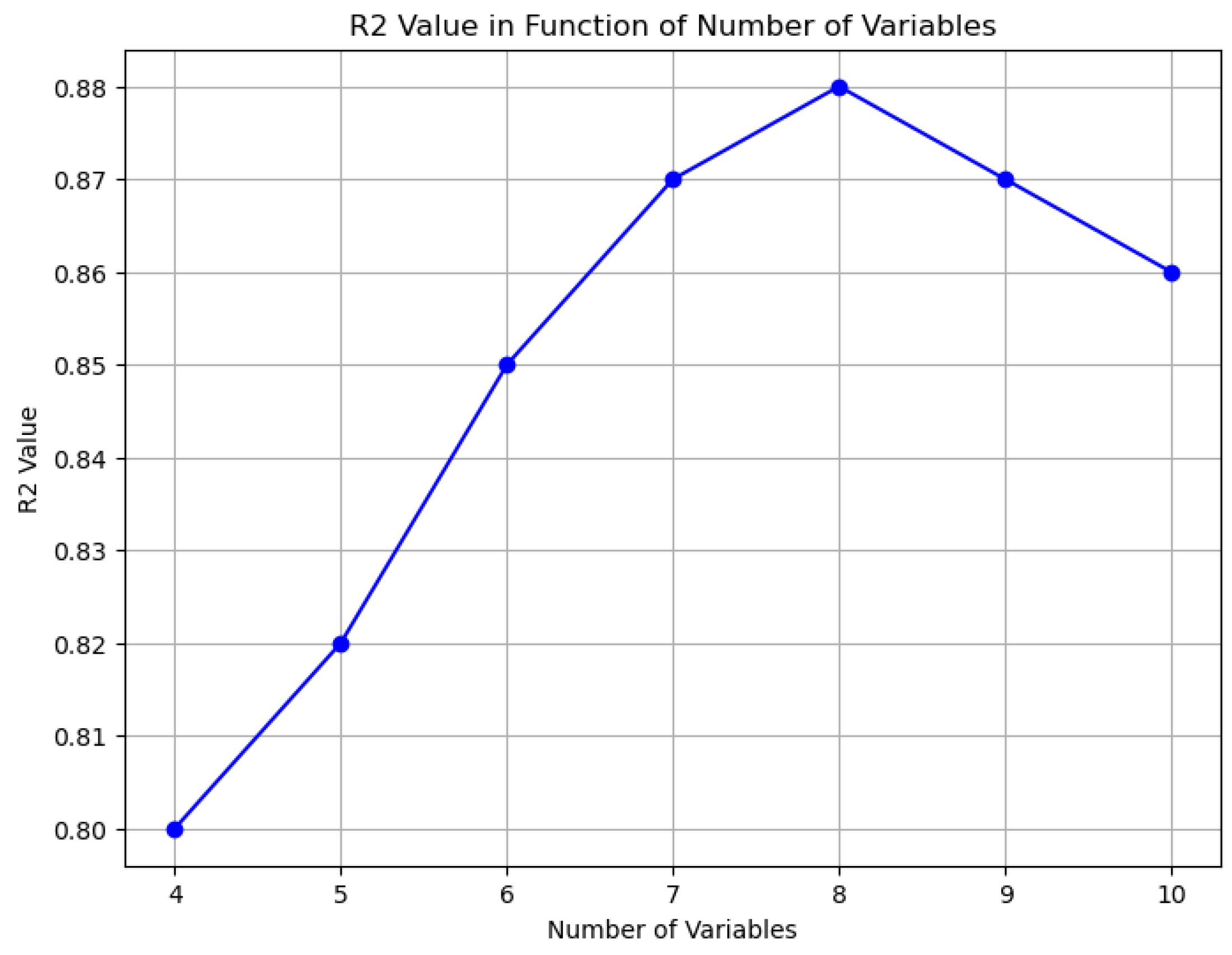
A sensitivity analysis was conducted to evaluate how the value of R2 changes with the number of variables in the Random Forest model and the results were shown in the following graph (
Figure 11). The radar diagram (
Figure 12) was also produced, which provides a clear and immediate view of the relative importance of variables in the model. Together, these diagrams provide a comprehensive understanding of the model’s performance, both in terms of individual variable contributions and overall model improvement.
Figure 12 illustrates the trend of model accuracy (measured by R
2) as a function of the number of explanatory variables. This analysis is theoretical and simulates the progressive inclusion of additional variables, some of which are hypothetical and not explicitly listed in the manuscript, to evaluate the model’s sensitivity to increasing complexity. The curve shows that accuracy improves with the addition of relevant variables up to a certain point (around eight variables), after which further additions lead to marginal gains or even slight decreases due to the potential introduction of noise or redundancy.
It is important to note that this analysis is not based on data from individual monitoring stations, but on spatially distributed variables applied across the study area. The graph in
Figure 11 represents a behavior in which the accuracy of the model (measured by R
2) increases with the addition of relevant variables up to a certain point, after which the addition of additional variables does not lead to significant improvements and may even cause a slight decrease in accuracy due to the introduction of noise or irrelevant variables. The radar diagram (
Figure 12), in addition to highlighting the relative importance of the variables, clearly showing which factors have the greatest impact on flood risk forecasts, shows the constancy of the R2 value considering all the variables together. It also suggests that the model is effective in predicting flood risk based on these variables.
A flood susceptibility map (FSM) is a crucial tool for spatial flash flood risk assessment. This map was generated using the Random Forest (RF) model, which represents a systematic approach for flood risk assessment within the study area. The risks were classified into four distinct categories: “low”, “moderate”, “high”, and “very high”, which were associated with distinct colors to identify the level of risk (
Figure 13).
Figure 13 shows the spatial distribution of flood susceptibility across the study area, as predicted by the Random Forest model. The model assigns a risk level to each cell of a regular grid based on the values of multiple spatial predictors (e.g., slope, land use, precipitation, drainage density). These predictions are then visualized in QGIS, where the classified risk levels are mapped using a color scale. The contour lines (isohypses) are included for topographic reference only and do not influence the classification. The resulting map highlights areas with varying degrees of flood susceptibility, not limited to the main river corridor. This spatially continuous output provides a valuable tool for identifying critical zones and supporting regional flood risk management strategies.
The green areas, being elevated or well-drained, have a low flood risk, while the yellow zone, characterized by moderate drainage, poses a moderate risk. The orange areas, typically near rivers or in flat, low-lying regions, face a high flood risk, and the red areas are very vulnerable, often requiring preventive measures. This scheme indicates that regions with low slopes in low-lying areas, especially those near river banks, are more susceptible to flash flooding [
41]. Given the number of high-risk zones, urgent flood risk management is essential, including infrastructure improvements, flood barriers, advanced warning systems, defined evacuation procedures, and potential restrictions on new construction.
Flood susceptibility plans are fundamental for spatial planning and disaster mitigation because they accurately map flood risk levels. This detailed information supports informed land management decisions such as building defense infrastructure, creating containment basins, and implementing effective drainage measures to protect people, property, and infrastructure while enhancing public safety. Moreover, informing local authorities and the public about flood risks leads to better resource allocation and coordinated interventions, which, when integrated with other planning tools like water management and urban planning, improve community resilience and reduce the impact of environmental disasters.
Performance Comparison of Random Forest and LSTM
In flood risk forecasting, it is crucial to utilize machine learning models that deliver accurate predictions while also capturing the underlying dynamics of the data. The model employed in this analysis was Random Forest (RF), validated through comparison with Long Short-Term Memory (LSTM), a model widely recognized for time series forecasting.
To ensure a comprehensive evaluation, the model performance was assessed using multiple metrics tailored to both regression and classification approaches. Specifically, Mean Squared Error (MSE), Root Mean Squared Error (RMSE), and R2 were employed to quantify the prediction error and explanatory power of the model, ensuring robust numerical evaluation of risk levels.
Additionally, given the ordinal nature of flood risk categories (low, moderate, high, very high), classification-oriented metrics were integrated, including accuracy, precision, recall, and F1-score. These indicators provide further insights into the model’s ability to correctly classify risk levels, addressing potential misclassifications between adjacent categories and reinforcing the reliability of the predictions.
This approach ensures that the continuous and categorical aspects of flood risk estimation are effectively captured, enhancing model interpretability and robustness.
Valuation metrics such as MSE, RMSE, and R
2 provide important insights into forecasting model performance. The comparison of the metric values between the two models, as shown in
Figure 14, revealed that the following:
The RF model’s mean squared error (MSE) is notably lower than that of the LSTM, indicating that RF makes fewer prediction errors. Similarly, the root mean squared error (RMSE) for RF is lower, confirming its higher accuracy. Moreover, the R-squared (R2) value for the RF model is slightly higher than that of the LSTM, suggesting that RF better explains the variance in the data.
In the light of the fact that more metrics were obtained, it was possible to make a detailed comparison between the Random Forest and LSTM models, the results of which are summarized in
Figure 15.
Accuracy: The Random Forest model (0.89) outperforms the LSTM (0.85), demonstrating a greater overall ability to correctly classify risk levels. This is particularly relevant in real-world scenarios, where any errors can have significant operational consequences.
Precision: Random Forest (0.91) exhibits higher accuracy than LSTM (0.88), reducing the likelihood of false alarms and helping to avoid unnecessary intervention.
Recall: Also in terms of sensitivity, Random Forest (0.87) proves to be more effective than LSTM (0.83), being more suitable for risk management, where it is essential not to underestimate situations of real danger.
F1-score: Random Forest (0.89) maintains a better balance between accuracy and recall than LSTM (0.84), making it more reliable in contexts where it is important to correctly balance false positives and false negatives.
Comparing the Random Forest (RF) and Long Short-Term Memory (LSTM) models, it becomes clear that the RF model significantly outperforms the LSTM regarding predictive accuracy. In the context analyzed, the Random Forest model proves to be more effective in classifying flood risk than the LSTM model.
The comparison between Random Forest and LSTM was conducted with the following three objectives in mind:
To verify the validity of the Random Forest model against a more advanced model like LSTM.
To identify the strengths and weaknesses of each model.
To determine the most suitable model for flood risk prediction in the context of this study.
The performance differences can be attributed to several factors. As an ensemble of decision trees, the RF model effectively captures interactions between variables and handles data variability. Decision trees excel at processing heterogeneous data and managing nonlinearity; characteristics often present in flood risk data. Moreover, RF is less sensitive to overfitting issues than LSTM, thanks to its ensemble nature, which averages predictions from many trees.
Another significant advantage of the RF model is its robustness and stability. Decision trees, the foundation of the RF model, are adept at handling noise and outliers in data. By combining predictions from multiple trees, the RF model further mitigates the impact of anomalies, making it particularly suitable for complex and noisy datasets like those used in flood risk forecasting.
RF’s versatility in handling different variables, be they categorical or numeric, without the need for complex transformations simplifies data preprocessing. This flexibility allows for a broader range of variables to be included in the model, enhancing its interpretability. The decisions made by the trees in the RF model are easily understandable, facilitating the comprehension of the relationships between variables and their impacts on predictions, thereby increasing the model’s transparency.
From a computational standpoint, the RF model is generally more efficient than the LSTM. Despite its complexity, implementing RF typically requires less computational resources and training time than LSTM, which demands larger datasets and more resources to train effectively. This makes RF a more practical and cost-effective choice for numerous applications.
On the other hand, while the LSTM model is robust in capturing time dependencies in data, its limitations can hinder its performance. LSTM may be more prone to overfitting, particularly with smaller datasets or highly correlated variables. Furthermore, the complexity of LSTM can complicate hyperparameter optimization, adversely affecting its ability to generalize well on test data.
In conclusion, the RF model is the superior choice for flood risk forecasting. Its ability to handle variability, robustness, ease of interpretation, and computational efficiency contribute to its superior performance over the LSTM model. This underscores the importance of selecting the right model based on the data’s characteristics and the analysis’s objectives.
A combined model could leverage Random Forest’s robustness and interpretability while utilizing LSTM’s ability to manage long-term dependencies, leading to more accurate predictions.
This combined approach could improve forecast accuracy and provide a more comprehensive understanding of flood risk dynamics. The integration of the two models could be achieved through ensemble learning techniques, where the predictions of both models are combined for a more robust final result. Additionally, employing stacking methods could enable predictions from one model to serve as input for the other, enhancing overall performance. This perspective represents an exciting opportunity for research and development in flood risk forecasting, with the potential to deliver more effective and reliable tools for risk management and mitigation.
6. Discussion
The results obtained demonstrate that the proposed approach, based on the integration between Random Forest and Markov chains, represents a significant step forward in flood risk prediction. The model showed high predictive performance, with an R
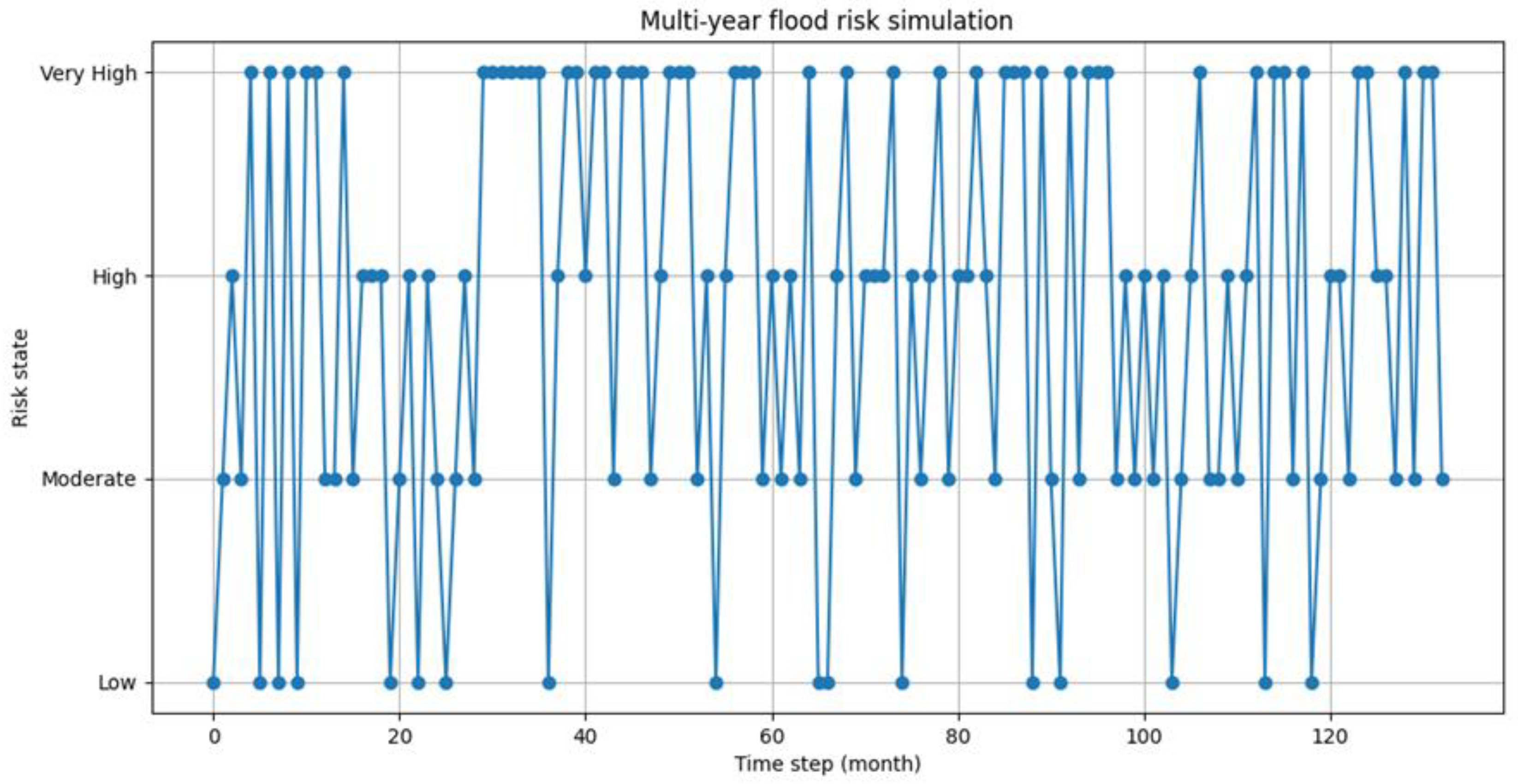
2 of 0.80 and a very low mean squared error (MSE) (0.014), even surpassing an LSTM model used as a reference. These results confirm the validity of the initial objective of the research: to develop a predictive system that was accurate, interpretable, and capable of modeling the temporal dynamics of risk. A distinctive element of our work is the use of the Markov chain to simulate the evolution of risk over time, as illustrated in
Figure 16. This figure, entitled “Simulated Flood Risk Fluctuations Over Time”, represents the temporal evolution of the simulated flood risk through the integration of the Random Forest model with a Markov chain. The simulation was generated starting from an initial state of low risk and iteratively applying the transition matrix calculated from the model predictions. Each time step represents one month, and the entire simulation covers a span of 11 years (132 months), offering a dynamic view of the evolution of risk over time.
Analyzing the results, we observe that the “High” and “Very High” risk states are the most common, accounting for 28.57% and 25.56% of the time, respectively. This indicates a higher overall frequency of elevated flood risk states in the simulation, though no clear temporal trend is visually evident in the time series. In contrast, the “Low” risk status is the least common, representing only 20.30% of the observations. A transition matrix governs the transitions between the risk states. For instance, from the “Low” state, there is a 27.78% chance of moving to either the “High” or “Very High” state. This highlights that even when the risk is low, there is a significant possibility of a rapid increase in risk.
The graph also illustrates monthly fluctuations among the different risk states, indicating considerable variability in flood risk every month. This variability suggests that the risk can change quickly from one month to the next, emphasizing the importance of continuous monitoring.
The figure does not have forecasting purposes, but provides a probabilistic representation useful for strategic purposes, to support the planning of risk mitigation interventions. The time series shows high monthly variability, with frequent transitions between all four risk states (“Low”, “Moderate”, “High”, and “Very High”). Although no net visual trend emerges, the aggregate analysis shows that the “High” and “Very High” states become predominant over time suggesting that, in the absence of interventions, the territory could be subject to an escalation of hydrogeological risk.
The original contribution of this study is divided into three main aspects: (1) the synergistic integration between machine learning models and stochastic models, (2) the use of high-resolution LIDAR data for the generation of digital terrain models, and (3) the ability of the model to provide both spatial and temporal predictions of risk. In particular, the use of LIDAR data with altimetric accuracy of less than 15 cm has made it possible to obtain an extremely detailed topographic representation, superior to that offered by low-resolution digital terrain models commonly used in the literature. This significantly improved the quality of spatial risk classification. In addition, direct comparison with an LSTM model highlighted the higher accuracy of our approach, which resulted in superior predictive metrics with a simpler and more interpretable computational structure. Finally, temporal modeling using Markov chains added a dynamic dimension to the analysis, making it possible to simulate the evolution of risk over time and to support long-term strategic decisions.
This approach not only improves the accuracy of forecasts but also expands the possibilities of operational use of the model, making it a useful tool for early warning systems, spatial planning, and emergency management.
In conclusion, our model does not limit itself to classifying areas at risk, but provides a dynamic and adaptive view of the flood phenomenon, contributing significantly to the evolution of hydrogeological risk forecasting and management tools.
6.1. Comparison with Other Methodologies
The findings underscore the importance of a modeling approach that not only achieves high predictive accuracy but also fosters strong interpretability and actionable insights. In this context, the comparison with other hydrogeological risk prediction methodologies demonstrates how the proposed model effectively balances precision, transparency, and flexibility. It successfully addresses the limitations of more complex approaches, such as LSTM, SVM, and CNN, as discussed below.
In terms of performance, the proposed model achieves excellent results in both classification and regression metrics. Comparisons with algorithms commonly used in the literature further validate the effectiveness of this approach. For instance, while LSTM neural networks are designed to capture time dependencies in sequential data, they exhibit lower performance compared to our model. Similarly, Support Vector Machines (SVMs) and Convolutional Neural Networks (CNNs) show significant limitations.
SVMs can be helpful in linear scenarios or when a well-chosen kernel is applied, but they struggle with heterogeneous and complex datasets, such as those arising from environmental and geospatial contexts. Furthermore, SVMs often lack interpretability, making it difficult to understand the contribution of individual variables to risk predictions. Studies, such as that by Granata et al. [
42], have indicated that while SVMs can effectively model urban runoff, they require careful calibration and might not perform well in dynamic scenarios.
On the other hand, CNNs excel in image processing but require substantial amounts of data and high computational resources. They are not inherently designed to model temporal components of risk unless paired with more complex architectures, such as CNN-LSTMs, which further complicate the system. A study by Wang et al. [
41] utilized CNNs for flood susceptibility mapping; however, the results demonstrated lower interpretability and flexibility compared to tree-based models, such as Random Forest.
In contrast, the proposed model maintains an optimal balance between accuracy, efficiency, and transparency. By utilizing LIDAR data to generate digital terrain models (DTMs), it ensures superior spatial accuracy. Additionally, stochastic modeling through Markov chains enables the simulation of risk evolution over time. This approach not only enhances the quality of forecasts but also serves as a valuable tool for spatial planning and emergency management.
Even when compared to hybrid approaches present in the literature, such as the one proposed by Kim et al. [
43], which combines LSTM and Random Forest for urban flood risk forecasting, the model stands out due to its ease of implementation and greater transparency in decision-making. While Kim’s model necessitates complex numerical simulations to generate training data, the approach used here is grounded in observational and geospatial data, making it more replicable and adaptable to different geographical contexts.
In summary, the proposed model is a robust, advanced, and adaptable solution that effectively overcomes the limitations of existing methodologies, providing a concrete contribution to flood risk management in the face of increasing climate vulnerability.
6.2. The Limitations, Scalability, and Adaptability of the Model
The model was developed and validated using data from a single catchment, the Calopinace River basin in Reggio Calabria. This choice was guided by the availability of high-resolution LIDAR data, detailed land use and lithological maps, and a consistent 11-year meteorological dataset. The basin’s complex topographic and urban characteristics provided a suitable testbed for methodological development.
However, the use of a single basin limits the spatial generalizability of the results. The absence of spatial cross-validation across multiple watersheds or hydroclimatic regimes restricts the assessment of model robustness under varying environmental conditions.
The current study is intended as a proof-of-concept to demonstrate the methodological soundness of the RF–Markov framework. Future research will focus on extending the model to additional catchments in southern Italy, characterized by diverse geomorphological and climatic features.
Moreover, regional climate models, which use historical and current climate data to simulate future weather patterns, are essential for assessing the impacts of climate change at a local scale and for developing effective mitigation strategies.
A limitation of the present study lies in the absence of georeferenced historical flood event data for the Calopinace River basin. While several major flood events have been documented (e.g., 1951, 1953, 1972, 2000, 2015), these records are primarily qualitative or aggregated at the municipal level, lacking the spatial resolution required for pixel-level validation. Consequently, a direct comparison between model predictions and historical flood extents was not feasible.
To address this constraint, we adopted a proxy-based validation strategy grounded in real environmental predictors such as LIDAR-derived elevation, lithology, land use, and long-term rainfall averages and applied Principal Component Analysis (PCA) to derive a synthetic flood susceptibility index. This index, classified into four ordinal risk levels, served as a statistically robust and reproducible proxy for flood risk in the absence of empirical flood labels.
The model’s performance metrics (RMSE = 0.118, MSE = 0.014, R2 = 0.80), obtained via 3-fold cross-validation, reflect its internal consistency and generalization capacity within the study area. While these metrics do not represent real-world predictive accuracy in the strictest sense, they provide a reliable internal benchmark given the available data.
Despite this limitation, the model offers practical value for decision-makers operating in data-scarce environments. It provides a spatially explicit, interpretable, and reproducible framework for identifying areas of high environmental susceptibility to flooding, supporting proactive land use planning and early warning systems.
Future work will focus on accessing and digitizing historical flood archives in collaboration with local authorities and civil protection agencies. This will enable more direct validation and the potential integration of event-based calibration techniques to further enhance model reliability. Finally, to further improve predictive capacity, combining the Random Forest algorithm with LSTM neural networks which excel at processing sequential and temporal data may capture long-term dependencies in climate and hydrological data. This combination promises to enhance flood risk forecasts, making the model more robust and adaptable to varying regional conditions.


