A Multibody Model Calibration Method for Vehicle Misuse Testing

Abstract

This paper proposes a multibody model calibration method for vehicle misuse testing. During misuse tests conducted at high driving speeds, the vehicle’s responses can become highly nonlinear due to certain key model parameters. Direct calibration using a complex multibody model is time-consuming and unstable, as it may fail or diverge due to improper settings of the model parameters. Therefore, a modified quarter-vehicle model is proposed for the analytical calibration of these nonlinear parameters by introducing an additional constraint on the sprung mass to recover the restoring force. The new model features only two degrees of freedom and incorporates key nonlinear parameters, including the suspension’s stiffness and the wheel’s center mass. It is suitable for misuse tests involving tire detachment at high driving speeds. The detailed analytical calibration procedure for the nonlinear parameters is deduced and subsequently validated through numerical simulation using these parameters. When the parameters are sufficiently close to the actual ones or linearly related to the responses, an optimization method such as the least squares method can be applied, along with simulations using complex models in commercial software.

1. Introduction

Misuse tests are crucial for verifying chassis performance and safety in vehicle engineering. They typically involve driving vehicles at high speeds over road obstacles such as speed bumps, deep potholes, square ridges, etc. [1]. Through testing under these extreme driving conditions, critical chassis components can be identified and subsequently optimized.

Vehicle dynamics models [2] can expedite misuse analyses and optimization of critical components [3]. Generally, the initial dynamics model is constructed using designed vehicle data. Once the model is calibrated with field-test data, it can be used for subsequent virtual simulations to optimize the critical chassis components [4]. This approach eliminates the need for repeated manufacturing of damaged and optimized components, as well as repeated preparation for field tests.

However, calibrating vehicle dynamics models is significantly more challenging in misuse tests than in durability tests [5]. As depicted in Figure 1, parameter differences between the tested and designed vehicles may arise from chassis tuning for comfort and clearance, test preparation, and damaged-part replacement. Road obstacles are significantly larger during misuse tests. At high driving speeds, the dynamic responses of displacements, acceleration, and forces are typically highly nonlinear with respect to certain vehicle parameters [6,7].

The state of the art in vehicle misuse tests involving vehicle dynamics models has been summarized in

Table 1. The state of the art in vehicle misuse tests involving vehicle dynamics models.

Items		Garcia-Pozuelo [9]	Zhang [8]	Guo [7]	Haerian [6]	Zhou [5]	Yin [10]	Presented
Years		2014	2020	2022	2022	2023	2024	2025
Obstacles h(×l if given) (cm × cm)	Bump	10 × 90	-	6 × 50	13 × 500	-	5.8 × 37	10 × 46
	Groove	-	-	-	6 × 74	-	-	-
	Curb	-	-	-	14	10	-	-
	Pothole	-	4.5 × 50	-	-	-	5.8 × 37	-
	Sleeper	-	10 × 7.5	-	7 × 15	-	-	-
Driving Speed (km/h)	Bump	70	-	20	55	-	40	40~60
	Groove	-	-	-	50	-	-	-
	Curb	-	-	-	15	50	-	-
	Pothole	-	80	-	-	-	40	-
	Sleeper	-	30	-	36	-	-	-
Vehicle Type (Num. of Wheels)		Car (4)	Car (4)	Car (4)	Motorcycle (2)	Car (4)	Car (4)	Car (4)
Suspension	Spring Type	Helical	Helical	Helical	Helical	Helical	Helical	Air
	Damper Type	Passive	Passive	Passive	Semi-active	Passive	Passive	Passive
Vehicle Model	Analytical Model	Planar full car	-	L-V coupling full-car model	Full motorcycle model	-	Quarter-car model	Modified quarter-car mode
	Software	-	Abaqus /Explicit	-	Adams /Car	Adams /Car	Carsim	Adams /Car
Tire Contact Model		Point contact	FE tire	Finite radial springs	FTire	FTire	Point contact	FTire/ Point contact
Response Direction	Longitudinal	-	√	√	√	√	-	√
	Vertical	√	√	√	√	√	√	√
	Pitch	-	-	√	-	-	-	√
	Lateral	-	-	-	-	-	-	-
Calibration Method		-	-	-	-	-	Genetic algorithm	Analytical+ least square

, along with the case that will be presented in this paper for comparison. In the existing literature, driving speeds exceeding 60 km/h have typically only been considered in the context of small obstacles [8] or gradual road obstacles [9]. For severe obstacles, the driving speed is lower, typically ranging from 15 km/h to 50 km/h, as indicated in references [5,6,7,8,10]. Suspensions are mainly equipped with helical springs, including some references that have used semi-active dampers [6]. No suspensions with air springs have been reported in misuse tests. The vehicles tested have mainly been four-wheel passenger cars, with the exception of one study focusing on a two-wheel motorcycle [6].

Regarding misuse vehicle modeling, multibody dynamics software such as Adams/Car [5,6] and Carsim [10] are primarily utilized, while the finite element software Abaqus/Explicit [8] is occasionally employed. For contact detection between vehicles and road obstacles, tire models must be applied. Adams/Car usually utilizes the Ftire model, while Carsim commonly employs a point-contact tire model. Abaqus/Explicit, on the other hand, naturally adopts a finite element tire model. However, vehicle misuse simulations in commercial software are often laborious, involving time-consuming modeling, calculation, and post-processing stages. Consequently, analytical multibody dynamics models [6,7,9,10] are frequently introduced and executed prior to commercial software calculations and/or as an alternative in control algorithms. In analytical modeling, the point contact model and the finite radial spring model are commonly used due to their ease of implementation and calculation using MATLAB/Simulink, as demonstrated in references [6,7,9]. The most concerning response directions are the vertical and longitudinal directions, followed by the pitch and lateral directions.

In Table 1, only reference [10] details an application of a genetic algorithm to calibrating the vehicle model parameters in misuse tests. Indeed, intelligent algorithms cannot always be applied fully automatically, as improper vehicle parameters may result in failures or divergences within the calculations by commercial software. Therefore, artificial intervention during the optimization process may be necessary. In addition, the responses may be highly nonlinear with respect to uncalibrated vehicle parameters [6,7], such as the axle weight, wheel-hub mass, spring stiffness, damper damping, stopper gap, etc. Only when the model parameters are very close to the actual parameters can iteration-based methods converge effectively.

The traditional quarter-vehicle model has been widely used to simulate vehicle misuse. Florin [11] detailed the quarter-vehicle solution process using MATLAB. Hassaan [12] used the quarter-vehicle model to simulate passage over a harmonic bump. Masino [13] utilized it to estimate road conditions using data mining methods and vehicle-based sensors. Alim [14] combined it with homotopy perturbation and frequency–amplitude methods to analyze the vibrations of a vehicle crossing over a speed bump in recent research.

Various types of tire models have been proposed and utilized in vehicle misuse simulations for vehicle–ground contact simulations. Hanley modeled a tire using finite element methods for misuse scenarios. Gipser [15] proposed the widely used Ftire model for all applications related to vehicle dynamics. Schmeitz [16] proposed the semi-empirical rigid ring tire model for misuse cases, as well as effective height and enveloping models for obstacle contact. Kim [17] proposed a two-dimensional analytical tire model for uneven roads, which consisted of a rigid ring, a six-degrees-of-freedom (6-DOF) spring/damper element, a static circular beam, and radial residual springs. Oertel [18] proposed the RMOD-K 7 tire model for bump and slope pit cases at speeds ranging from 30 to 60 km/h. Baecker [19] used CDTire during severe events with significant tire deformations, where the response amplitudes coincided well, with some error in the vibration periods. Linden [20] studied the influence of the wheel’s bending stiffness on the lateral tire characteristics during misuse tests. Liu [21] proposed a coupled rigid–flexible ring model for simulations on uneven roads. Some tire models were compared in the review by Zhang [22].

Vehicle misuse simulations have been applied in various aspects of vehicle design and improvement. Messana [23] obtained a lightweight design for a multi-material suspension lower control arm. Qin [24] a designed hydropneumatic suspension system for a road–rail vehicle. Leister [25] designed a mobility system for damaged tires and wheels for mobility recovery. Kersten [26] assessed the controllability after chassis component damage using a dynamic driving simulator. Li [27] evaluated the strength performance of the steering system in hybrid off-road vehicles.

This paper proposes a multibody model calibration method for vehicle misuse tests conducted at high driving speeds and using severe obstacles. A modified quarter-vehicle model is proposed for misuse test calibration, incorporating an additional equivalent spring between the sprung mass and an imagined ceiling to restore the force recovery. By considering various tire contact statuses, the process of passing over an obstacle is segmented into three stages and analyzed sequentially. Once the model’s parameters closely align with those for the tested vehicle, the least squares method is utilized to achieve precise results.

This paper is structured as follows: Section 2 presents the overall calibration workflow using commercial software. Here, actual vehicle experiment data are compared against simulation results derived from complex models within commercial software. Subsequently, the parameter sensitivity is calculated, and the model is optimized using the least squares method for linear parameters, as elaborated in Section 3. Section 4 offers a detailed description of the proposed modified quarter-vehicle model, encompassing the analytical calibration method for nonlinear response parameters. The process of the vehicle traversing over a speed bump at high speed is divided into three stages: the obstacle contact stage, the tire detachment stage, and the ground recontact stage. The dynamic characteristics of each stage are theoretically analyzed to calibrate the nonlinear parameters. Subsequently, the validity of the model and method is confirmed through numerical simulation using the calibrated parameters, leading to the conclusion in Section 5.

2. The Overall Calibration Workflow with Commercial Software

In this section, we present an overall calibration workflow that utilizes commercial software for vehicle misuse tests. The workflow, detailed in Section 2.1, primarily consists of three parts: the test processes for the prototype vehicle, complex multibody simulations in Adams(2023)/Car, and a collaborative theoretical auxiliary analysis process. The corresponding simulation model, settings, and parameters for calibration within Adams/Car are introduced in Section 2.2.

2.1. The Overall Calibration Workflow

The overall calibration workflow for vehicle misuse tests is illustrated in Figure 2. Starting from the designed vehicle parameters, the full processes are mainly divided into three phases: (a) road tests of the real vehicle, (b) calibration loops using virtual simulation in Adams/Car, and (c) a theoretical auxiliary analysis using the modified quarter-vehicle model.

During the road test phase, the vehicle is tuned, loaded, tested, and recorded. Chassis tuning should be conducted before testing to ensure the chassis is in the optimal condition for daily use. In the Class II tests, the chassis is raised by an additional 30 mm to facilitate passage over deep potholes. This tuning results in variations in the air spring stiffness, shock absorber damping, and the stopper gap. The loads also need to be adjusted from a half-load to a full-load counterweight for the misuse tests, as the initial vehicle model is typically designed for durability analyses under the former conditions. Next, the altered vehicle is tested by passing over various obstacles at a given speed, and the responses are recorded using sensors and outputted in *.s3t format, which can be processed using experimental data software, such as nCode(11.1).

During the Adams/Car calibration phase, the detailed multibody model is built, simulated, compared, and adjusted. As described above, the Adams/Car model was initially built for durability analyses. Simulating on virtual ground with the given obstacles, as depicted in Figure 3, the numerical results are output in *.rsp format to be read in nCode as well. The simulation results are compared with the test results, and the errors in both the amplitudes and the periods are assessed. If the errors are small, the parameter sensitivity is calculated using the finite difference method, with additional simulations for parameter perturbation. Subsequently, assuming a linear input–output relationship, the vehicle parameters are adjusted using the least squares optimization method. The simulation loop continues until the errors are found to have converged, at which point the calibration process is concluded.

If the errors are large or medium, the input–output relation may become highly nonlinear. Improper setting of the vehicle parameters may result in simulation failure or divergences in Adams/Car, interrupting the parameter iteration loop. In this case, the theoretical analysis is necessary to help calibrate a set of parameters that are sufficiently close to initiate the iteration. As depicted in the workflow in Figure 2, the theoretical analysis method proposes a modified quarter-vehicle model and divides the misuse process into three stages: obstacle contact, free detaching, and ground recontact. Contact and modal analyses are conducted theoretically to calibrate the vehicle parameters by comparing the response amplitudes and periods, a process that will be detailed in subsequent subsections.

2.2. Misuse Test Simulation with Commercial Software

Figure 3 depicts an Adams/Car simulation of the vehicle misuse test where the vehicle passes over a speed bump on a digital road surface. As with the road tests, the time domain responses are recorded. As displayed in

Table 2. Vehicle responses, measurement channels, and corresponding model parameters.

Responses	Description	Measurement Channels	Corresponding Model Parameters
$v$	Driving speed	GPS sensor	Driving speed $v$
$f_{\mathrm{z}}$	The vertical wheel’s center force	Six-component force meter (only used for Class I obstacles)	The vehicle’s total mass $m$, the vehicle’s moment of inertia $J$, the centroid position $(x,y)$
${\ddot{z}}_{\mathrm{w}}$	The wheel’s center acceleration in the z (vertical) direction	Acceleration sensor	The shock absorber’s stiffness $k_{\mathrm{s}}$, damping $c_{\mathrm{s}}$, preload $f_{\mathrm{s}}$, the wheel’s center mass $m_{\mathrm{w}}$
$d$	Shock absorber compression	Cable displacement sensor

, the recorded responses primarily include the driving speed $v$, the vertical wheel center force ${\mathit{f}}_{\mathrm{z}}$, the vertical wheel center acceleration $a_{\mathrm{z}}$, the shock absorber compression $d_{\mathrm{s}}$, and the lower control arm tension $f_{\mathrm{c}}$. With these responses, the vehicle’s driving posture and force distribution are essentially defined. The driving speed can be measured using a GPS sensor, the vertical wheel center force using a six-component force meter, the accelerations using acceleration sensors at a specific positions, the shock absorber compression using a cable displacement sensor, and the arm tensions using strain gauges attached to the components. It is notable that the six-component force meter is utilized exclusively for Class I obstacles and not for Class II obstacles. Class I obstacles include speed bumps [19,28,29,30] and square roadblocks. Class II obstacles include square potholes and slope potholes, with the chassis clearance being 30 mm higher than that for Class I obstacles.

The road test responses allow for calibration of the corresponding model parameters, which are listed in the third column of Table 2. In other words, these parameters directly affect the respective responses. For instance, the recorded driving speed $v$ is itself a model parameter. The vertical wheel’s center force $f_{\mathrm{z}}$ is determined by the vehicle’s total mass $m$, the moment of inertia $J$, and the centroid position $(x,y)$. The subsequent analysis reveals a strong correlation between the vertical wheel’s center acceleration ${\ddot{z}}_{\mathrm{w}}$ and the shock absorber compression $d$, both of which are determined by the shock absorber’s stiffness $k_{\mathrm{s}}$, the damping $c_{\mathrm{s}}$, the preload $f_{\mathrm{s}}$, and the wheel’s center mass $m_{\mathrm{w}}$. Although the GPS sensor records altitude changes, it does not calibrate the vehicle’s vertical height due to its measurement error, which can be as large as 0.1 m.

It is important to note that measurement channels that have failed should be identified and excluded from the experimental data. Sensor failure occurs more frequently in misuse tests than in durability tests due to the harsh response in the vehicle components when they come into contact with obstacles at high driving speeds.

3. Linear Parameter Calibration Using the Least Squares Method

In this section, a linear parameter calibration process utilizing the least squares method is presented for vehicle misuse testing. Certain vehicle parameters, such as its mass and centroid position, exhibit a nearly linear relationship with their corresponding responses. This process can also be applied to nonlinear parameters, provided they are sufficiently close to the actual vehicle values. The calibration process for the vehicle’s mass and centroid position is described in this section as an example.

The vehicle’s mass and centroid position must be calibrated for misuse tests. Generally, the design department can only supply an Adams/Car (or any other vehicle simulation software) model with a half-load counterweight, initially set up for durability analyses. However, misuse tests typically require a full-load counterweight configuration.

To calibrate the vehicle’s mass and centroid position using road test data, the wheel loads are initially calculated from the experimental responses on a flat road segment, as shown in Figure 4a. Prior to encountering the obstacle, the vehicle must maintain a specified speed on the flat road segment. The six-component force meters record the forces acting on the wheel centers, including the vertical forces. Then, the averages of the vertical forces are considered as the loads acting on each wheel—for instance, ${\overline{f}}_{\mathrm{RF}}$ on the right front wheel, ${\overline{f}}_{\mathrm{LF}}$ on the left front wheel, ${\overline{f}}_{\mathrm{RR}}$ on the right rear wheel, and ${\overline{f}}_{\mathrm{LR}}$ on the left rear wheel. For the target vehicle discussed in this paper, the wheel loads are 6.5 kN, 7 kN, 8 kN, and 8 kN, respectively, as indicated in Figure 4b. In fact, these values indicate a discrepancy between the rigid chassis model and the actual vehicle chassis. To explain this, it is hypothesized that the rigid chassis’s descent height $\mathrm{\Delta }h$, caused by the loads, exhibits a bilinear relationship with respect to the chassis’s local longitudinal coordinates $\xi$ and lateral coordinates $\eta$ as follows:

$$\mathrm{\Delta }h=a\xi +b\eta +c.$$

(1)

wherein $a$ and $b$ represent the longitude slope and the lateral slope, respectively, and $c$ is the average descent height of the four wheels.

In the vehicle examined in this paper, the air springs of the front wheels differ from those of the rear wheels both in structure and stiffness. Therefore, let $k_{\mathrm{F}}$ and $k_{\mathrm{R}}$ denote the suspension stiffness of the front and rear wheels, respectively. The reaction force function can be given through Lagrange interpolation as

$$f(\xi ,\eta )=[k_{\mathrm{R}}+{\displaystyle \frac{\xi -{\xi }_{\mathrm{R}}}{{\xi }_{\mathrm{F}}-{\xi }_{\mathrm{R}}}}(k_{\mathrm{F}}-k_{\mathrm{R}})]\left(a\xi +b\eta +c\right),$$

(2)

wherein ${\xi }_{\mathrm{F}}$ and ${\xi }_{\mathrm{R}}$ represent the local longitudinal coordinates of the front and rear wheels, respectively. The force difference between the two front wheels is

$$\mathrm{\Delta }{f}_{\mathrm{F}}=f({\xi }_{\mathrm{F}},{\eta }_{\mathrm{L}})-f({\xi }_{\mathrm{F}},{\eta }_{\mathrm{R}})=k_{\mathrm{f}}\left(a{\xi }_{\mathrm{F}}+b{\eta }_{\mathrm{L}}+c\right)-k_{\mathrm{f}}\left(a{\xi }_{\mathrm{F}}+b{\eta }_{\mathrm{R}}+c\right)=k_{\mathrm{F}}b({\eta }_{\mathrm{L}}-{\eta }_{\mathrm{R}}),$$

(3)

and the force difference between the two rear wheels is

$$\mathrm{\Delta }{f}_{\mathrm{R}}=f(x_{\mathrm{R}},{\eta }_{\mathrm{L}})-f(x_{\mathrm{R}},{\eta }_{\mathrm{R}})=k_{\mathrm{r}}\left(a{x}_{\mathrm{R}}+b{\eta }_{\mathrm{L}}+c\right)-k_{\mathrm{R}}\left(a{x}_{\mathrm{R}}+b{\eta }_{\mathrm{R}}+c\right)=k_{\mathrm{R}}b({\eta }_{\mathrm{L}}-{\eta }_{\mathrm{R}}).$$

(4)

Formulas (3) and (4) illustrate that both $\mathrm{\Delta }{f}_{\mathrm{F}}$ and $\mathrm{\Delta }{f}_{\mathrm{R}}$ are either zero or non-zero simultaneously. However, the recorded average forces of the rear wheels are the same, whereas those of the front wheels are not. This discrepancy reflects the difference between the rigid chassis model and the actual vehicle chassis, due to flexible deformation of the chassis.

By applying the least squares method, the descent height parameters $a$, $b$, and $c$ can be calibrated. However, in practice, the vehicle’s mass $m$ and centroid position $(x,y)$ are used instead of the descent height parameters. On the one hand, $c$ is directly influenced by $m$, while $a$ and $b$ are influenced by $(x,y)$; on the other hand, utilizing $m$ and $(x,y)$ can circumvent the impact of the suspension stiffness on the results.

The actual vehicle experiment data (test data) are taken as the target, and we start with the simulation results for the initial parameters. The parameter sensitivity is computed using the finite difference method, with significant variations $\mathrm{\Delta }m=100 \mathrm{kg}$, $\mathrm{\Delta }x=100 \mathrm{mm}$, and $\mathrm{\Delta }y=100\mathrm{mm}$ to suppress numerical errors in the Adams/Car simulation. As depicted in

Table 3. Calibration of the vehicle’s mass and centroid position using the least squares method: four-wheel load data for the target, the initial model, and the variant models; that predicted using the least squares method; and that for the simulated model (∆m = 100 kg, ∆x = ∆y = 100 mm); the value unit is kN.

Wheel Position	Tested (Test Data)	Initial	Initial +∆m	Initial +∆x	Initial +∆y	Predicted Using Least Squares	Calibrated
	${\mathit{f}}_{\mathrm{test}}$	${\mathit{f}}_0$	${\mathit{f}}_1$	${\mathit{f}}_2$	${\mathit{f}}_3$	${\mathit{f}}_{\mathrm{pred}}$	${\mathit{f}}_{\mathrm{cali}}$
Left Front (LF)	7.03	6.50	6.74	6.22	5.84	6.95	6.93
Right Front (RF)	6.52	6.50	6.74	6.22	7.15	6.59	6.49
Left Rear (LR)	8.00	6.88	7.11	7.16	6.47	8.12	8.20
Right Rear (RR)	8.00	6.88	7.11	7.16	7.30	7.89	7.93

, the sensitivity matrix $\mathit{A}$ with respect to the parameters ${[m,x,y]}^{\mathrm{T}}$ can be computed according to the quotient between the column’s differences and the variation as

$$\mathit{A}=\left[\begin{array}{ccc}{\mathit{f}}_1-{\mathit{f}}_0& {\mathit{f}}_2-{\mathit{f}}_0& {\mathit{f}}_3-{\mathit{f}}_0\end{array}\right]/100.$$

(5)

Then, with the response error

$$e={\mathit{f}}_0-{\mathit{f}}_{\mathrm{test}},$$

(6)

the predicted parameters are computed as

$${\left[m_{\mathrm{c}},x_{\mathrm{c}},y_{\mathrm{c}}\right]}^{\mathrm{T}}={\left[m_0,x_0,y_0\right]}^{\mathrm{T}}+{({\mathit{A}}^{\mathrm{T}}\mathit{A})}^{-1}{\mathit{A}}^{\mathrm{T}}\mathit{e}.$$

(7)

With the calibrated parameters ${\left[m_{\mathrm{c}},x_{\mathrm{c}},y_{\mathrm{c}}\right]}^{\mathrm{T}}$, the Adams/Car simulation results $f_{\mathrm{cali}}$ are very close to the actual data from the vehicle experiment (test data), as shown in Figure 5 and Table 3.

4. Nonlinear Parameter Calibration Using the Modified Quarter-Vehicle Model Analysis

For vehicle parameters that exhibit strong nonlinearity with respect to their dynamic responses, analytical models and methods are essential to determine the initial calibration values. During misuse tests involving traversal over a relatively large speed bump at high speeds, detachment of the tires from the road’s surface is a fundamental characteristic.

In this section, the obstacle negotiation process is divided into three distinct stages: the obstacle contact stage, the tire detachment stage, and the ground recontact stage. The traditional quarter-vehicle model has been adapted to this specific misuse scenario by incorporating an imaginary recovery spring between the sprung mass and an imaginary fixed ceiling. This modification allows the differential equations with two degrees of freedom for the three stages to be theoretically solved, albeit partially. However, this is sufficient to calibrate the unknown vehicle parameters. The process of solving these equations and calibrating the nonlinear parameters is detailed in this section.

4.1. The Modified Quarter-Vehicle Model

Calibration of the shock absorber’s stiffness and the wheel’s center mass is crucial for vehicle misuse tests. These parameters directly influence the responses of the shock absorber compression $d(t)$ and the wheel’s center acceleration ${\ddot{z}}_{\mathrm{w}}(t)$ (in units of standard gravitational acceleration $g$), as depicted in Figure 6b. In the driving attitude, the compression reflects the relative position from the wheel center to the vehicle body, while the acceleration indicates the absolute position of the wheel center determined through two rounds of time integration.

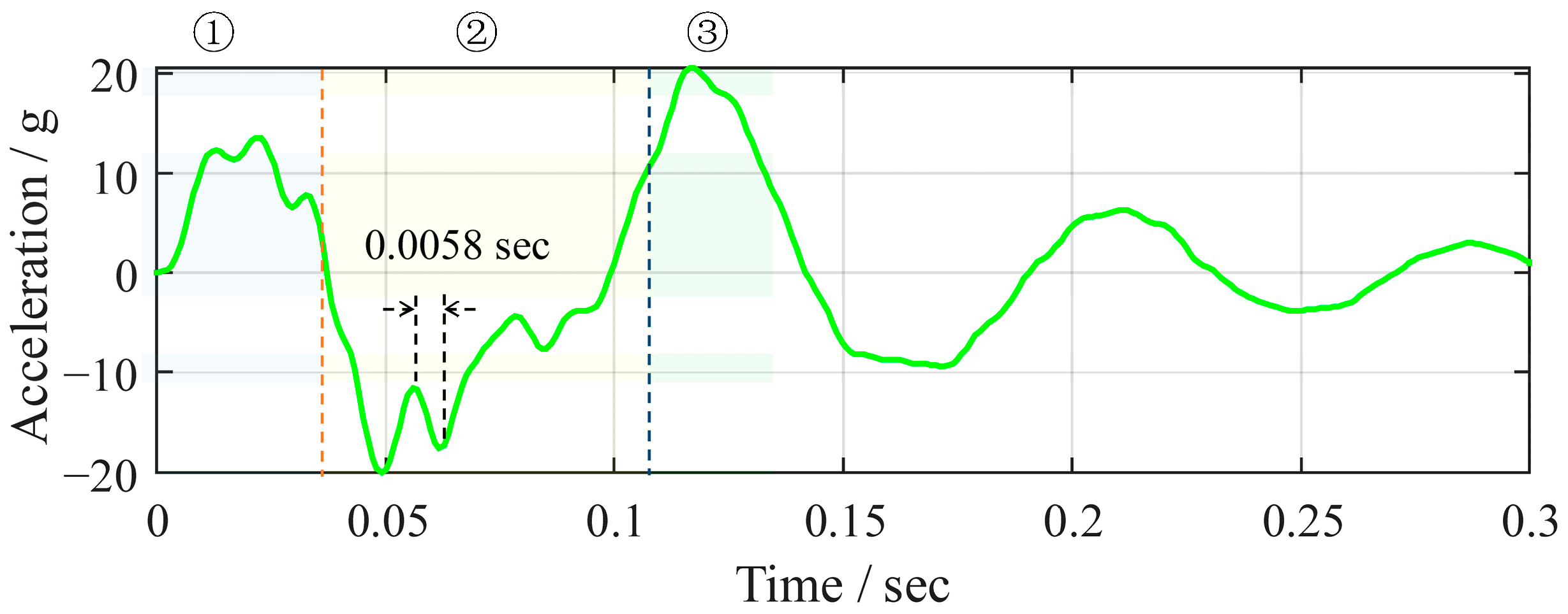
When the vehicle passes over relatively large obstacles at high speeds, the shock absorber’s compression and the wheel center’s acceleration exhibit strong nonlinearity. This is caused by discontinuous changes in the tire–ground contact conditions, which are subsequently reflected in the vehicle’s responses. The contact process is naturally divided into three stages on the timeline, as depicted in Figure 6a: ① $t_1\le t<t_2$, the obstacle contact stage; ② $t_2\le t<t_3$, the tire detachment stage; and ③ $t_3\le t$, the ground recontact stage. The contact status between the tire and the road varies distinctly in these three stages, presenting different dynamic characteristics that result in complex, nonlinear responses.

To analyze the three distinct stages in the process of passing over the speed bump, a modified quarter-vehicle model is proposed in this paper. As depicted in Figure 6c, compared to the traditional quarter-vehicle model used in durability and smoothness tests, an equivalent spring $k_{\mathrm{e}}$ is added between the sprung mass and an imagined ceiling.

The force generated by the equivalent spring represents a “recovery force”. This force originates from the suspension springs and tires at the opposite end of the vehicle and is transferred through the chassis via pitch motion. For instance, when the front wheels of a vehicle traverse over a convex obstacle, the front end of the vehicle is lifted, creating an angle of elevation. If the height of the chassis center is assumed to remain constant, the rear end will descend, and the rear suspension will produce a recovery force to counteract the pitch motion. The converse is also true. Consequently, the equivalent spring maintains the influence of the suspension on the opposite end in the modified quarter-vehicle model. Furthermore, in this manner, the front and rear suspensions are decoupled. With only two degrees of freedom (DOFs) in the modified quarter-vehicle model, it is much easier to theoretically analyze the three distinct stages simultaneously, a task that is significantly more challenging for a half-vehicle model [9] with four DOFs.

Given the brief duration of the contact process, the gravitational force can be disregarded in the theoretical analyses. This model accounts for tire damping, consistent with the references [11,12], whereas it is neglected in others [13,14]. Indeed, the subsequent numerical simulation in Section 4.5 will demonstrate that the tire’s damping ratio is essential to the comparison with the actual vehicle experiment data (test data). In the context of the current misuse scenario, the tire damping is significant, particularly because of the pronounced vehicle response at high driving speeds.

The scheme between $t_2$ and $t_3$ indicates that the tire detaches from the road’s surface during this interval, where the two-DOF system responds in the form of excited free vibration. Since the tire’s mass is neglected in the present paper, the tire spring is inactive during this stage and is represented in gray.

In the modified quarter-vehicle model, the variables are the vertical displacements of the sprung point and the wheel’s center, namely $z_{\mathrm{u}}$ and $z_{\mathrm{w}}$. The front wheels and the rear wheels are decoupled from their respective equivalent stiffness $k_{\mathrm{e}}$. In the following three subsections, the differential equations for each stage will be analyzed in detail. The sequence progresses from stages ② to ③ and then to ①, not in the order of progression, but rather from simple to complex, to determine the vehicle parameters.

4.2. Equivalent Stiffness Calibration by Tire Detaching Stage

It will be demonstrated that the modified model can effectively replicate the obstacle contact process with the equivalent stiffness $k_{\mathrm{e}}$ and thus yield a practical misuse analysis method.

Firstly, the displacement relationship between the sprung mass and the wheel’s center is examined. With the wheel’s center acceleration recorded during the tests, the wheel center’s vertical displacement is computed by integrating twice with respect to time $t$ as

$$z_{\mathrm{w}}(t)={\displaystyle {\int }_0^t({\displaystyle {\int }_0^t{\ddot{z}}_{\mathrm{w}}}\left(\mathrm{t}\right)\mathrm{d}t)}\mathrm{d}t.$$

(8)

Comparing the numerical result from Equation (8) with the shock absorber’s compression response $d(t)$ depicted in Figure 7, an approximate quantitative relationship is identified for the current vehicle as

$$d(t)\approx 0.73\times z_{\mathrm{w}}(t).$$

(9)

Because the shock absorber is nearly vertical, with the compression distance relation

$$d(t)\approx z_{\mathrm{w}}(t)-z_{\mathrm{u}}(t),$$

(10)

the vertical displacements of the sprung point is obtained as

$$z_{\mathrm{u}}(t)\approx 0.27\times z_{\mathrm{w}}(t)$$

(11)

or in the vibration mode formulation as

$$\left[\begin{array}{c}{z}_{\mathrm{u}}(t)\\ z_{\mathrm{w}}(t)\end{array}\right]\approx \left[\begin{array}{c}0.27\\ 1\end{array}\right]z_{\mathrm{w}}(t).$$

(12)

Relation (9) (also Equation (12)) is particularly well satisfied in stage ②, as depicted in Figure 7. In stage ②, the tire detaches from the obstacle, and the wheel’s center vibrates vertically under the action of the shock absorber’s force. Ignoring the constant gravitational forces, the vibration modes in stage ② can be computed using the following eigen equations:

$$\left[\begin{array}{cc}{m}_{\mathrm{u}}& 0\\ 0& m_{\mathrm{w}}\end{array}\right]\left[\begin{array}{c}{\ddot{z}}_{\mathrm{u}}(t)\\ {\ddot{z}}_{\mathrm{w}}(t)\end{array}\right]+\left[\begin{array}{cc}{k}_{\mathrm{e}}+k_{\mathrm{s}}& -k_{\mathrm{s}}\\ -k_{\mathrm{s}}& k_{\mathrm{s}}\end{array}\right]\left[\begin{array}{c}{z}_{\mathrm{u}}(t)\\ z_{\mathrm{w}}(t)\end{array}\right]=0,$$

(13)

wherein $m_{\mathrm{u}}\ge 0$ represents the sprung mass, $m_{\mathrm{w}}$ represents the wheel’s center mass, $k_{\mathrm{e}}\ge 0$ represents the equivalent stiffness of the recovery force, and $k_{\mathrm{s}}$ represents the suspension spring’s stiffness. Since the tire’s mass is neglected in the present paper and the lower end of the tire spring detaches from the ground in this stage, no excitation of the ground is caused by the tire. Consequently, no term related to $k_{\mathrm{t}}$ appears in Equation (13). This stage responds as a free vibration with an initial speed and a position at the lower end.

To simplify Equation (13), let $c_{\mathrm{u}}=m_{\mathrm{u}}/m_{\mathrm{w}}\ge 0$, $c_{\mathrm{e}}=(k_{\mathrm{e}}+k_{\mathrm{s}})/k_{\mathrm{s}}\ge 1$, and divide the equation by $m_{\mathrm{w}}$ to obtain

$$\left[\begin{array}{cc}{c}_{\mathrm{u}}& 0\\ 0& 1\end{array}\right]\left[\begin{array}{c}{\ddot{z}}_{\mathrm{u}}(t)\\ {\ddot{z}}_{\mathrm{w}}(t)\end{array}\right]+{\displaystyle \frac{k_{\mathrm{s}}}{m_{\mathrm{w}}}}\left[\begin{array}{cc}{c}_{\mathrm{e}}& -1\\ -1& 1\end{array}\right]\left[\begin{array}{c}{z}_{\mathrm{u}}(t)\\ z_{\mathrm{w}}(t)\end{array}\right]=0,$$

(14)

Let ${\omega }_0^2=k_{\mathrm{s}}/m_{\mathrm{w}}$ and hypothesize that the solution is $\left[\begin{array}{c}{z}_{\mathrm{u}}(t)\\ z_{\mathrm{w}}(t)\end{array}\right]=\mathit{z}\cdot \sin (\omega t+\phi )$ with the eigenmode $\mathit{z}$, the circular frequencies $\omega$, and the initial phase angle $\phi$; the following algebraic equation is obtained:

$$\left\{-{\omega }^2\left[\begin{array}{cc}{c}_{\mathrm{u}}& 0\\ 0& 1\end{array}\right]+{\omega }_0^2\left[\begin{array}{cc}{c}_{\mathrm{e}}& -1\\ -1& 1\end{array}\right]\right\}\mathit{z}=0.$$

(15)

Solving Equation (15) yields the eigenvectors as

$${\mathit{z}}_{\pm }=\left[\begin{array}{c}{\displaystyle \frac{(c_{\mathrm{u}}-c_{\mathrm{e}})\pm \sqrt{{(c_{\mathrm{u}}-c_{\mathrm{e}})}^2+4c_{\mathrm{u}}}}{2c_{\mathrm{u}}}}\\ 1\end{array}\right].$$

(16)

The corresponding eigen circular frequencies are

$${\omega }_{\pm }^2={\displaystyle \frac{(c_{\mathrm{u}}+c_{\mathrm{e}})\mp \sqrt{{(c_{\mathrm{u}}-c_{\mathrm{e}})}^2+4c_{\mathrm{u}}}}{2c_{\mathrm{u}}}}{\omega }_0^2,$$

(17)

wherein ${\omega }_{+}^2=0$ only if $c_{\mathrm{e}}=1$.

For the traditional quarter-vehicle model without, i.e., the synclastic eigenvector and frequency are, respectively,

$${\mathit{z}}_{+,\mathrm{f}}=\left[\begin{array}{c}1\\ 1\end{array}\right]\mathrm{with} {\omega }_{+,\mathrm{f}}^2=0,$$

(18)

and in the opposite direction, they are, respectively,

$${\mathit{z}}_{-,\mathrm{f}}=\left[\begin{array}{c}-{\displaystyle \frac{1}{c_{\mathrm{u}}}}\\ 1\end{array}\right]\mathrm{with} {\omega }_{-,\mathrm{f}}^2=\left(1+{\displaystyle \frac{1}{c_{\mathrm{u}}}}\right){\displaystyle \frac{k_{\mathrm{s}}}{m_{\mathrm{w}}}}.$$

(19)

Mode results (18) and (19) show that in the traditional quarter-vehicle model, synclastic vibration of $z_{\mathrm{u}}$ and $z_{\mathrm{w}}$ only happens in the rigid-body movement (18). Therefore, the traditional quarter-vehicle model is not applicable to the misuse tests. However, with $c_{\mathrm{e}}>1$ in the modified quarter-vehicle model, Formula (16) gives the synclastic eigenmode with $z_{\mathrm{u}}$ and $z_{\mathrm{w}}$ as

$$z_{+,②}=\left[\begin{array}{c}{\displaystyle \frac{(c_{\mathrm{u}}-c_{\mathrm{e}})+\sqrt{{(c_{\mathrm{u}}-c_{\mathrm{e}})}^2+4c_{\mathrm{u}}}}{2c_{\mathrm{u}}}}\\ 1\end{array}\right],$$

(20)

with the corresponding non-zero circular frequency

$${\omega }_{+,②}^2=\left({\displaystyle \frac{(c_{\mathrm{u}}+c_{\mathrm{e}})-\sqrt{{(c_{\mathrm{u}}-c_{\mathrm{e}})}^2+4c_{\mathrm{u}}}}{2c_{\mathrm{u}}}}\right){\displaystyle \frac{k_{\mathrm{s}}}{m_{\mathrm{w}}}}.$$

(21)

Let $c_{②}\triangleq z_{\mathrm{u}}/z_{\mathrm{w}}$ be the ratio of the synclastic displacements of the sprung mass and the wheel center in stage ②; Equation (20) suggests

$${\displaystyle \frac{(c_{\mathrm{u}}-c_{\mathrm{e}})+\sqrt{{(c_{\mathrm{u}}-c_{\mathrm{e}})}^2+4c_{\mathrm{u}}}}{2c_{\mathrm{u}}}}=c_{②},$$

(22)

so solving this and abandoning the unreasonable solution ($z_{\mathrm{u}}=0$), the ratio $c_{\mathrm{e}}$ is expressed by the ratio $c_{\mathrm{u}}$ as

$$c_{\mathrm{e}}=(1-c_{②})c_{\mathrm{u}}+{\displaystyle \frac{1}{c_{②}}},$$

(23)

and substituting Equation (22) into Equation (21), the ratio between the suspension spring’s stiffness and the wheel’s center mass is written as

$${\displaystyle \frac{k_{\mathrm{s}}}{m_{\mathrm{w}}}}={\displaystyle \frac{{\omega }_{+,②}^2}{1-c_{②}}}.$$

(24)

In the present vehicle, $c_{②}=0.27$ is read from the result (12), and it produces $c_{\mathrm{e}}=0.73c_{\mathrm{u}}+3.70$.

It is important to note that only the synclastic mode is activated during stage ②. Given that the obstacle impact force originates from one side of the mass–spring system, specifically from the tire side, the opposing mode remains inactive. This is evidenced by the alignment of the displacement curve during the half-period of 0.0675 s in stage ②, as illustrated in Figure 7. One might also wonder whether the rapid vibration component of the acceleration response indicates the opposing eigenmode with a higher frequency. However, the answer is no, and the detailed proof is provided in Appendix A.

4.3. Tire Stiffness Calibration by Ground Recontact Stage

After stage ②, the tire makes contact with the road again, causing vibrations in the suspension to generate stage ③. By adding the tire stiffness $k_{\mathrm{t}}$ depicted in Figure 6c, the equation for the modified quarter-vehicle model of stage ③ is

$$\left[\begin{array}{cc}{m}_{\mathrm{u}}& 0\\ 0& m_{\mathrm{w}}\end{array}\right]\left[\begin{array}{c}{\ddot{z}}_{\mathrm{u}}(t)\\ {\ddot{z}}_{\mathrm{w}}(t)\end{array}\right]+\left[\begin{array}{cc}{k}_{\mathrm{e}}+k_{\mathrm{s}}& -k_{\mathrm{s}}\\ -k_{\mathrm{s}}& k_{\mathrm{s}}+k_{\mathrm{t}}\end{array}\right]\left[\begin{array}{c}{z}_{\mathrm{u}}(t)\\ z_{\mathrm{w}}(t)\end{array}\right]=\left[\begin{array}{c}0\\ 0\end{array}\right].$$

(25)

In stage ③, the excitation of the ground is transmitted through the tire stiffness $k_{\mathrm{t}}$ to the system. To simplify this expression, the corresponding term is moved to the left side and incorporated into the stiffness matrix in Equation (25). Let $c_{\mathrm{t}}=(k_{\mathrm{t}}+k_{\mathrm{s}})/k_{\mathrm{s}}\ge 1$, and because $c_{\mathrm{u}}=m_{\mathrm{u}}/m_{\mathrm{w}}\ge 0$, Equation (25) can be rewritten as

$$\left[\begin{array}{cc}{c}_{\mathrm{u}}& 0\\ 0& 1\end{array}\right]\left[\begin{array}{c}{\ddot{z}}_{\mathrm{u}}(t)\\ {\ddot{z}}_{\mathrm{w}}(t)\end{array}\right]+{\displaystyle \frac{k_{\mathrm{s}}}{m_{\mathrm{w}}}}\left[\begin{array}{cc}{c}_{\mathrm{e}}& -1\\ -1& c_{\mathrm{t}}\end{array}\right]\left[\begin{array}{c}{z}_{\mathrm{u}}(t)\\ z_{\mathrm{w}}(t)\end{array}\right]=\left[\begin{array}{c}0\\ 0\end{array}\right].$$

(26)

Similarly to the vibration solution in Equation (16), in stage ③, the following synclastic eigenmode is generated as

$$z_{+,③}=\left[\begin{array}{c}{\displaystyle \frac{(c_{\mathrm{t}}\hspace{0.17em}{c}_{\mathrm{u}}-c_{\mathrm{e}})+\sqrt{{(c_{\mathrm{t}}{c}_{\mathrm{u}}-c_{\mathrm{e}})}^2+4\hspace{0.17em}{c}_{\mathrm{u}}}}{2\hspace{0.17em}{c}_{\mathrm{u}}}}\\ 1\end{array}\right],$$

(27)

and the synclastic circular frequency for stage ③

$${\omega }_{+,③}^2=\left({\displaystyle \frac{(c_{\mathrm{t}}\hspace{0.17em}{c}_{\mathrm{u}}+c_{\mathrm{e}})-\sqrt{{(c_{\mathrm{t}}\hspace{0.17em}{c}_{\mathrm{u}}-c_{\mathrm{e}})}^2+4c_{\mathrm{u}}}}{2c_{\mathrm{u}}}}\right){\displaystyle \frac{k_{\mathrm{s}}}{m_{\mathrm{w}}}}.$$

(28)

Comparing Equation (28) with Equation (21) yields

$${\displaystyle \frac{{\omega }_{+,②}^2}{{\omega }_{+,③}^2}}={\displaystyle \frac{(c_{\mathrm{u}}+c_{\mathrm{e}})-\sqrt{{(c_{\mathrm{u}}-c_{\mathrm{e}})}^2+4c_{\mathrm{u}}}}{(c_{\mathrm{t}}\hspace{0.17em}{c}_{\mathrm{u}}+c_{\mathrm{e}})-\sqrt{{(c_{\mathrm{t}}\hspace{0.17em}{c}_{\mathrm{u}}-c_{\mathrm{e}})}^2+4c_{\mathrm{u}}}}}={\displaystyle \frac{2c_{\mathrm{u}}{c}_{②}}{(c_{\mathrm{t}}\hspace{0.17em}{c}_{\mathrm{u}}+c_{\mathrm{e}})-\sqrt{{(c_{\mathrm{t}}\hspace{0.17em}{c}_{\mathrm{u}}-c_{\mathrm{e}})}^2+4c_{\mathrm{u}}}}},$$

(29)

or rewritten as

$$(c_{\mathrm{t}}\hspace{0.17em}{c}_{\mathrm{u}}+c_{\mathrm{e}})-\sqrt{{(c_{\mathrm{t}}\hspace{0.17em}{c}_{\mathrm{u}}-c_{\mathrm{e}})}^2+4c_{\mathrm{u}}}={\displaystyle \frac{2c_{\mathrm{u}}{c}_{②}{\omega }_{+,③}^2}{{\omega }_{+,②}^2}}.$$

(30)

We solve the upper algebraic equation to obtain

$$c_{\mathrm{t}}={\displaystyle \frac{-c_{\mathrm{u}}\hspace{0.17em}{c}_{②}^2\hspace{0.17em}{\omega }_{+,③}^4+c_{\mathrm{e}}\hspace{0.17em}{c}_{②}\hspace{0.17em}{\omega }_{+,②}^2\hspace{0.17em}{\omega }_{+,③}^2+{\omega }_{+,②}^4}{c_{\mathrm{e}}\hspace{0.17em}{\omega }_{+,②}^4-c_{\mathrm{u}}\hspace{0.17em}{c}_{②}\hspace{0.17em}{\omega }_{+,②}^2{\omega }_{+,③}^2}}.$$

(31)

Upon examining Figure 7, it is evident that for the tested vehicle, ${\omega }_{+,②}={\displaystyle \frac{2\pi }{T_{②}}}={\displaystyle \frac{2\pi }{2 \times 0.0675 \mathrm{s}}}=46.54 \mathrm{rad}/\mathrm{s}$ and ${\omega }_{+,③}={\displaystyle \frac{2\pi }{T_{③}}}={\displaystyle \frac{2\pi }{2 \times 0.0340 \mathrm{s}}}=92.40 \mathrm{rad}/\mathrm{s}$, and thus $c_{\mathrm{t}}=3.86$.

4.4. Equivalent Obstacle Parameter Calibration by Obstacle Contact Stage

As depicted in Figure 6, in comparison to the model from stage ③, the lower point of the tire spring ascends as the vehicle moves forward in stage ①. Considering the potential nonlinearity in the actual tire response, an equivalent method to that presented by Zegelaar in the reference [31] is adopted for the speed bump’s geometry. Instead of an equivalent shape to that in the reference [31], it is assumed that the lower end moves upward with an equivalent vertical velocity $v_{\mathrm{e}}$. Then, the obstacle contact process is described by the following equation (ignoring gravity):

$$\left[\begin{array}{cc}{m}_{\mathrm{u}}& 0\\ 0& m_{\mathrm{w}}\end{array}\right]\left[\begin{array}{c}{\ddot{z}}_{\mathrm{u}}(t)\\ {\ddot{z}}_{\mathrm{w}}(t)\end{array}\right]+\left[\begin{array}{cc}{k}_{\mathrm{e}}+k_{\mathrm{s}}& -k_{\mathrm{s}}\\ -k_{\mathrm{s}}& k_{\mathrm{s}}+k_{\mathrm{t}}\end{array}\right]\left[\begin{array}{c}{z}_{\mathrm{u}}(t)\\ z_{\mathrm{w}}(t)\end{array}\right]=\left[\begin{array}{c}0\\ k_{\mathrm{t}}{v}_{\mathrm{e}}t\end{array}\right].$$

(32)

The difference between stage ① and stage ③ is that the former features a slope on the speed bump. When the tire rolls onto the slope, the ground ascends relative to the wheel’s center. Therefore, in addition to the term $k_{\mathrm{t}}$ on the left side, as seen in Equation (25), there is an additional excitation force $k_{\mathrm{t}}{v}_{\mathrm{e}}t$ on the right side due to the “ascending” ground.

Divide the two sides by $m_{\mathrm{w}}$, and use the relation $c_{\mathrm{t}}=(k_{\mathrm{t}}+k_{\mathrm{s}})/k_{\mathrm{s}}$, $c_{\mathrm{e}}=(k_{\mathrm{e}}+k_{\mathrm{s}})/k_{\mathrm{s}}$; the above equation is simplified as

$$\left[\begin{array}{cc}{c}_{\mathrm{u}}& 0\\ 0& 1\end{array}\right]\left[\begin{array}{c}{\ddot{z}}_{\mathrm{u}}(t)\\ {\ddot{z}}_{\mathrm{w}}(t)\end{array}\right]+{\displaystyle \frac{k_{\mathrm{s}}}{m_{\mathrm{w}}}}\left[\begin{array}{cc}{c}_{\mathrm{e}}& -1\\ -1& c_{\mathrm{t}}\end{array}\right]\left[\begin{array}{c}{z}_{\mathrm{u}}(t)\\ z_{\mathrm{w}}(t)\end{array}\right]={\displaystyle \frac{k_{\mathrm{t}}}{m_{\mathrm{w}}}}\left[\begin{array}{c}0\\ v_{\mathrm{e}}t\end{array}\right].$$

(33)

When an effort is made to solve the two-DOF equation theoretically using Laplace transformation, the expression of the result becomes somewhat complex, making it difficult to extract the necessary information for calibration. Therefore, a single-DOF vibrational model, as depicted in Figure 8, is considered to extract useful information from its theoretical solution.

The equivalence is as follows: If two systems have the same natural frequencies, modes, and boundary conditions, their responses will be identical, and thus they will be equivalent. If the main response components of the original system can be preserved in a system with fewer DOFs, then the latter can be regarded as a simplified version of the original system. In fact, only one of the two modes in the two-DOF mass–spring system has principally been excited by the slope of the speed bump. This can be illustrated by the frequency and mode analyses in Equations (16) and (17), where the natural frequencies and directions of motion are distinct for the two modes. Only the synclastic mode is likely to be excited; the opposite cannot be the main one. Therefore, with the same boundary conditions at the lower end and the same natural frequency, the single-DOF vibrational model can be considered a simplification of the original two-DOF system.

For the model in Figure 8 with the mass $m$, the structural spring stiffness $k$, and the tire stiffness $k_{\mathrm{t}}$, the system equation is written as

$$m\ddot{z}+(k+k_{\mathrm{t}})z=k_{\mathrm{t}}{v}_{\mathrm{e}}t.$$

(34)

Suppose the initial condition is $\ddot{z}(0)=\dot{z}(0)=0$; we apply the Laplace transformation [32] to Equation (34) and obtain

$$(m{s}^2+k+k_{\mathrm{t}})Z={\displaystyle \frac{k_{\mathrm{t}}{v}_{\mathrm{e}}}{s^2}},$$

(35)

wherein $Z(s)=\mathcal{L}(z(t))$ is the Laplace image of the displacement $z(t)$. With the natural circular frequency of the system ${\omega }_0=\sqrt{\left(k+k_{\mathrm{t}}\right)/m}$ with two springs, $Z$ is solved as

$$Z={\displaystyle \frac{k_{\mathrm{t}}{v}_{\mathrm{e}}}{s^2(m{s}^2+k+k_{\mathrm{a}})}}={\displaystyle \frac{k_{\mathrm{t}}{v}_{\mathrm{e}}}{m{s}^2(s^2+{\omega }_0^2)}}={\displaystyle \frac{k_{\mathrm{t}}{v}_{\mathrm{e}}}{m{\omega }_0^2}}\left({\displaystyle \frac{1}{s^2}}-{\displaystyle \frac{1}{s^2+{\omega }_0^2}}\right)={\displaystyle \frac{k_{\mathrm{t}}{v}_{\mathrm{e}}}{k+k_{\mathrm{t}}}}\left({\displaystyle \frac{1}{s^2}}-{\displaystyle \frac{1}{{\omega }_0}}{\displaystyle \frac{{\omega }_0}{(s^2+{\omega }_0^2)}}\right),$$

(36)

According to the relation $z(t)={\mathcal{L}}^{-1}(Z(s))$, the solution of the forced vibration is obtained as

$$z={\displaystyle \frac{k_{\mathrm{t}}{v}_{\mathrm{e}}}{k+k_{\mathrm{t}}}}\left(t-{\displaystyle \frac{1}{{\omega }_0}}\sin ({\omega }_{0}t)\right)=\left(1-{\displaystyle \frac{1}{c_{\mathrm{t}}}}\right)v_{\mathrm{e}}\left(t-{\displaystyle \frac{1}{{\omega }_0}}\sin ({\omega }_{0}t)\right).$$

(37)

The maximum acceleration of the mass is then

$${\ddot{z}}_{\max }=\left(1-{\displaystyle \frac{1}{c_{\mathrm{t}}}}\right)v_{\mathrm{e}}{\omega }_0.$$

(38)

The displacement $z(t)$ also occurs at the upper point of the tire spring. Therefore, in the modified quarter-vehicle model, we utilize the maximum acceleration of the wheel’s center as the value for ${\ddot{z}}_{\max }$ Equation (38) instead. As ${\omega }_0$ is the natural circular frequency of the system, we take ${\omega }_0={\omega }_{+,③}$ in the modified quarter-vehicle model instead. That is,

$$v_{\mathrm{e}}={\displaystyle \frac{{\ddot{z}}_{\max ,①}}{{\omega }_{+,③}}}\cdot {\displaystyle \frac{c_{\mathrm{t}}}{c_{\mathrm{t}}-1}}.$$

(39)

Upon examining the acceleration response curve for stage ① in Figure 6b, the current vehicle obtains ${\ddot{z}}_{\max ,①}\approx 12g$, where $g=9.8 \mathrm{m}/\mathrm{s}$ is the unit gravity acceleration. With $c_{\mathrm{t}}=3.86$ and ${\omega }_{+,③}=92.40 \mathrm{rad}/\mathrm{s}$, $v_{\mathrm{e}}=1.57 \mathrm{m}/\mathrm{s}$ is obtained. During the obstacle contact time interval of 0.035 s, the equivalent vertical displacement of the wheel’s center is 55 mm, which is 55% of the speed bump’s height.

4.5. Method Validation via Numerical Simulation

The complete progression of the present misuse scenario has been divided into three stages according to different tire–ground contact conditions, where stages ① through ③ are described by ODEs (32), (13), and (25), respectively. The systematic ODEs are summarized here in a combined formulation as follows:

$$\left[\begin{array}{cc}{m}_{\mathrm{u}}& 0\\ 0& m_{\mathrm{w}}\end{array}\right]\left[\begin{array}{c}{\ddot{z}}_{\mathrm{u}}(t)\\ {\ddot{z}}_{\mathrm{w}}(t)\end{array}\right]+\left[\begin{array}{cc}{k}_{\mathrm{e}}+k_{\mathrm{s}}& -k_{\mathrm{s}}\\ -k_{\mathrm{s}}& k_{\mathrm{s}}\end{array}\right]\left[\begin{array}{c}{z}_{\mathrm{u}}(t)\\ z_{\mathrm{w}}(t)\end{array}\right]=\left\{\begin{array}{l}\left[\begin{array}{c}0\\ k_{\mathrm{t}}{v}_{\mathrm{e}}t-k_{\mathrm{t}}{z}_{\mathrm{w}}(t)\end{array}\right], \mathrm{for} t_1\le t<t_2,\\ \left[\begin{array}{c}0\\ 0\end{array}\right], \mathrm{for} t_2\le t<t_3,\\ \left[\begin{array}{c}0\\ -k_{\mathrm{t}}{z}_{\mathrm{w}}(t)\end{array}\right], \mathrm{for} t_3\le t.\end{array}\right.$$

(40)

wherein $t$ represents the time variable; $z_{\mathrm{u}}(t)$ and $z_{\mathrm{w}}(t)$ represent the vertical displacement of the sprung mass and the wheel center, respectively; $m_{\mathrm{u}}$ represents the sprung mass; $m_{\mathrm{w}}$ represents the wheel’s center mass; $k_{\mathrm{s}}$ represents the suspension spring’s stiffness; $k_{\mathrm{t}}$ represents the tire’s stiffness; $k_{\mathrm{e}}$ represents the equivalent stiffness between the sprung mass and the imagined ceiling; and $v_{\mathrm{e}}$ represents the equivalent vertical velocity of the ground during tire–obstacle contact.

Divide the two sides by $m_{\mathrm{w}}$ and take $c_{\mathrm{u}}=m_{\mathrm{u}}/m_{\mathrm{w}}\ge 0$, $c_{\mathrm{e}}=(k_{\mathrm{e}}+k_{\mathrm{s}})/k_{\mathrm{s}}\ge 1$, and $c_{\mathrm{t}}=(k_{\mathrm{t}}+k_{\mathrm{s}})/k_{\mathrm{s}}\ge 1$, as in Section 4.2, Section 4.3 and Section 4.4; i.e., with the ODEs (33), (14), and (26), the systematic ODEs to be solved are combined as follows:

$$\left[\begin{array}{cc}{c}_{\mathrm{u}}& 0\\ 0& 1\end{array}\right]\left[\begin{array}{c}{\ddot{z}}_{\mathrm{u}}(t)\\ {\ddot{z}}_{\mathrm{w}}(t)\end{array}\right]+{\displaystyle \frac{k_{\mathrm{s}}}{m_{\mathrm{w}}}}\left[\begin{array}{cc}{c}_{\mathrm{e}}& -1\\ -1& 1\end{array}\right]\left[\begin{array}{c}{z}_{\mathrm{u}}(t)\\ z_{\mathrm{w}}(t)\end{array}\right]=\left\{\begin{array}{l}{\displaystyle \frac{k_{\mathrm{t}}}{m_{\mathrm{w}}}}\left[\begin{array}{c}0\\ v_{\mathrm{e}}t-z_{\mathrm{w}}(t)\end{array}\right], \mathrm{for} t_1\le t<t_2,\\ \left[\begin{array}{c}0\\ 0\end{array}\right], \mathrm{for} t_2\le t<t_3,\\ -{\displaystyle \frac{k_{\mathrm{t}}}{m_{\mathrm{w}}}}\left[\begin{array}{c}0\\ z_{\mathrm{w}}(t)\end{array}\right], \mathrm{for} t_3\le t.\end{array}\right.$$

(41)

In Equations (40) and (41), the nonlinearity resulting from varying tire–ground contact conditions is clearly evident and ultimately leads to nonlinearity in the vehicle’s response. The key parameters of the modified quarter-vehicle model, namely $c_{\mathrm{e}}$, $c_{\mathrm{t}}$, and $v_{\mathrm{e}}$, have been provided by Expressions (23), (31), and (38), respectively. Then, the systematic responses of the quarter-vehicle model can be computed using a time integration function in software, such as MATLAB(2022)’s ode15s, a numerical integration solver for stiff problems with 1–5-order polynomials, or MATLAB(2022)’s ode45, a widely used efficient solver for non-stiff problems using the Runge–Kutta method.

The systematic parameters for numerical simulation are listed in

Table 4. The systematic parameters of the modified quarter-vehicle model for numerical simulation.

Parameter	Value	Unit	Description
$c_{\mathrm{u}}$	10.00	-	$m_{\mathrm{u}}/m_{\mathrm{w}}$
$c_{②}$	0.27	-	$z_{\mathrm{u}}/z_{\mathrm{w}}$ in stage ②
$c_{\mathrm{e}}$	11.00	-	$(k_{\mathrm{e}}+k_{\mathrm{s}})/k_{\mathrm{s}}$
$c_{\mathrm{t}}$	3.86	-	$(k_{\mathrm{t}}+k_{\mathrm{s}})/k_{\mathrm{s}}$
$v_{\mathrm{e}}$	1.57	m/s	Equivalent vertical speed of the tire moving upwards
${\omega }_{+,②}$	46.54	rad/s	Circular frequency in stage ②
${\omega }_{+,③}$	92.40	rad/s	Circular frequency in stage ③
$t_2$	0.035	s	Time for which the tire disconnects from the obstacle
$t_3$	0.1023	s	Time for which the tire reestablishes contact with the ground
Damping ratio	0.002	N·s/m	Rayleigh damping proportional to the stiffness

, where a Rayleigh damping of 0.002, proportional to the stiffness, is added to the simulation model to obtain the damped results. The numerical results were computed using ode15s in MATLAB and subsequently compared with the actual vehicle experiment data (test data), as shown in Figure 9. For the shock absorber’s compression $d(t)$, the results are well coincident in stage ② and the initial part of stage ③.This is ensured by the calibration processes of the parameters $c_{\mathrm{e}}$$c_{\mathrm{t}}$, respectively. The results for the wheel’s center acceleration $\ddot{z}(t)$ are well coincident during the periods for stages ① through ③, but the simulation results exhibit smaller amplitudes than those in the tested data. More intense nonlinearity is observed in the test data, and fast vibration components with much higher frequencies than those in the simulated results are present in stages ① and ②. The fast component present in stage ① is primarily due to the tire deformation during and after contact with the obstacle. The simulation model does not include tire vibration, which accounts for the amplitude errors. The fast component present in stage ② primarily results from the contact with the stop-block, which serves to prevent excessive compression of the absorber. This element has not yet been incorporated into the simulation model. The simulation results show sudden changes in the wheel’s center acceleration at the specific moments $t_2$ and $t_3$, which are also evident in the corresponding curve for the test data.

In general, the simulation results maintain the fundamental characteristics of the misuse test data. As a result, the effectiveness of the proposed calibration method for vehicle misuse tests is validated. This method is particularly well suited to misuse tests involving high driving speeds, where the tire–ground detachment phase occurs. The absence of tire deformation vibrations and contact with the stop-block may result in inaccuracies in the wheel’s center acceleration response. Future work should also consider nonlinear stiffness to enhance the simulation accuracy.

5. Conclusions

In this paper, a novel multibody model calibration method for vehicle misuse testing is proposed, utilizing a modified quarter-vehicle model.

A severe obstacle contact process has been calibrated, where the experimental vehicle passed over relatively large speed bumps at high driving speeds and generated nonlinear responses. The complete process is divided into three stages because of the varying tire–ground contact conditions, rather than being a continuous progression influenced by minor road obstacles or slow driving speeds. The traditional quarter-vehicle model has been modified to adapt to severe misuse scenarios. An equivalent spring is added between the sprung mass and an imagined fixed ceiling to capture the recovery effect caused by the vehicle’s pitch motion. Then, the three-stage, two-degree-of-freedom ordinary differential equations are analyzed theoretically to calibrate the nonlinear vehicle parameters, even without proper initial values. The effectiveness of the presented modified quarter-vehicle model and the nonlinear parameter calibration method has been validated through numerical simulation using the calibrated parameters.

For parameter calibration involving nearly linear responses or appropriate initial values, the least squares method is employed. A comprehensive calibration workflow, encompassing actual vehicle experiments, commercial software simulation, and a theoretical analysis, is also introduced.

The proposed model does not account for tire deformation vibration, stop-block contact, or the nonlinearity of the suspension stiffness. Subsequent research may consider incorporating these factors into the modified quarter-vehicle model to enhance the simulation accuracy and obtain more precise calibrated parameters.