1. Introduction
At present, the two major problems facing human society are environmental pollution and the energy crisis. As awareness grows about the severity of environmental pollution and the transformation of economic society, countries around the world are seeking clean energy such as electricity, solar energy, and wind energy to address these issues [
1,
2].
The most widely used clean energy at present is electricity. With the popularization of electric vehicles, mobile devices, and renewable energy storage systems, the importance of lithium-ion batteries in various fields has become increasingly prominent [
3]. In the field of power batteries, lithium-ion batteries are core components of new energy vehicles, power tools, and electric bicycles, and their cost accounts for 30–40% of the total item cost [
4,
5]. With the continuous improvement of electric vehicle range and charging technology, higher requirements are also put forward for battery technology [
6]. The battery pack of electric vehicles is composed of hundreds to thousands of single cells in series, and the SOH difference between cells can lead to a decrease in energy utilization [
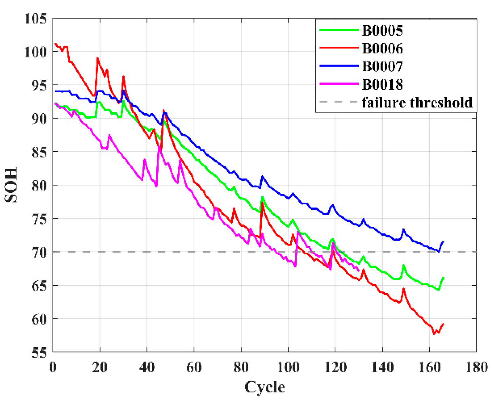
7]. For instance, if the capacity of a single cell degrades to 70%, the effective capacity of the entire battery pack will be limited by the “short board effect”, resulting in energy waste [
8]. At the same time, for end users, overcharging, over-discharging, or local overheating of the battery may cause thermal runaway, or even fire and explosion. As the battery ages, capacity decay will also cause a significant decrease in vehicle range. SOH prediction is not only a technical indicator of battery management but also a core link between safety, economy, and environmental protection. Real-time and accurate prediction of battery SOH is essential [
9].
Battery health state (SOH) is a core indicator for measuring battery performance degradation, usually defined as the ratio of the current maximum capacity or internal resistance to the initial value [
10]. At present, SOH estimation methods can be divided into model-based methods and data-driven methods, which have significant differences in principles, implementation, and applicable scenarios [
11]. First, the model-based method describes the internal dynamic process of the battery by establishing physical or electrochemical equations, and it uses the difference between observable external parameters (such as voltage, current, temperature) and model output to estimate the state. Its core is to associate the microscopic aging mechanism of the battery with the macroscopic behavior through mathematical modeling. There are two typical models: the electrochemical model and the equivalent circuit model. The principle of the electrochemical model is based on porous electrode theory (Pseudo-Two-Dimensional, P2D model), which describes the diffusion, insertion, or extraction process of lithium ions in positive and negative electrode materials by coupling mass conservation, charge conservation, and reaction kinetics equations [
12]. Its advantage lies in accurately characterizing the internal aging mechanism of the battery (such as SEI film growth and active material loss), which is suitable for mechanism research. However, the model has several disadvantages, including high model complexity (requiring the solution of high-dimensional partial differential equations), time-consuming calculations (with a single simulation taking several hours); difficulty in parameter identification (e.g., diffusion coefficients and reaction rate constants); and challenges in real-time online application. The principle of the equivalent circuit model is to use circuit elements such as resistors and capacitors to simulate the dynamic response of the battery [
13]. Common models usually include the following: (1) Rint model: only contains ohmic internal resistance; (2) Thevenin model: series RC network simulates polarization effect; (3) Dual Polarization (DP) model: dual RC network distinguishes between fast and slow polarization processes. The advantages and disadvantages of this model are also obvious. The advantage is that the calculation is simple (high real-time performance) and suitable for BMS online estimation [
14]. One disadvantage is that it cannot describe the internal aging mechanism of the battery and can only reflect the changes in macroscopic parameters. In order to solve the problem of inconsistency of electrochemical parameters caused by differences in battery manufacturing, Zhang et al. [
15] characterized individual differences through initial cycle state data and constructed a physical information dual neural network (PIDNN) to achieve dual functions: dynamic estimation of electrochemical parameters (such as lithium ion diffusion coefficient, reaction rate constant, etc.) and synchronous simulation of lithium ion concentration distribution in solid electrodes and electrolytes. The electrochemical model based on physical principles is combined with the deep learning model to break through the limitations of traditional data-driven methods that lack physical interpretability. It provides a new paradigm for SOH estimation with few samples, high precision, and clear interpretability. Liu et al. [
16] designed the battery physical information neural network (BatteryPINN) based on the mathematical model of solid electrolyte interface (SEI) film growth, and they embedded physical laws such as SEI film thickness evolution into the network structure. By explicitly modeling the SEI film growth process, the quantitative relationship between capacity decay and SEI film thickness is revealed, providing physical insights into the prediction results and overcoming the limitations of the “black box model”. In addition, the improved composite multi-scale Hilbert cumulative residual entropy algorithm is used to automatically extract high-quality health features directly from battery voltage and current data, providing a new idea for accurate, interpretable, and easy-to-deploy battery SOH estimation. Tran et al. [
17] continuously monitored Thevenin ECM (equivalent circuit model) parameters through cycle aging experiments and quantified their evolution with SOH degradation. After integrating the SOH factor, the voltage prediction error of the Thevenin model on the aged battery was reduced by about 40%, and the average accuracy of the whole life cycle was more than 99%. The system revealed the quantitative influence of SOH on Thevenin ECM parameters and realized the efficient prediction of ECM parameters under the synergy of multiple factors. It provided a core algorithm for adaptive ECM parameter update for smart BMS. Li et al. [
18] constructed an enhanced equivalent circuit model (ECMC) by adding capacitor elements to the classic ECM to improve the fitting ability of full-band EIS data. Optimization algorithms such as the nonlinear least squares method were used to identify ECMC model parameters and capture the evolution of parameters with battery aging. This provides a high-precision and highly adaptable SOH estimation scheme for BMS, particularly for actual working conditions under severe temperature fluctuations.
Compared with the above methods, the data-driven method analyzes the characteristics of battery aging cycle data in a simple way and establishes a relationship model between battery characteristics and SOH [
19]. The principle of the data-driven method is that the data-driven method abandons physical modeling and directly mines the statistical association between battery aging characteristics and SOH from historical data. The nonlinear mapping relationship between input (health features) and output (SOH) is constructed through machine learning algorithms [
20,
21]. The core steps of this data-driven model are health feature (HF) extraction, typical algorithm selection, and model training and verification. Among them, common traditional machine learning includes support vector regression (SVR): mapping high-dimensional space through kernel functions (such as RBF) to construct regression hyperplanes; random forests: integrating multiple decision trees to reduce the risk of overfitting. Deep learning includes long short-term memory networks (LSTM): capturing the temporal dependence of capacity decay; convolutional neural networks (CNNs): extracting local aging features from charge and discharge curve images [
22,
23,
24,
25]. The above models have the advantages of not requiring prior physical knowledge, adapting to complex nonlinear relationships, and being able to integrate multi-source data (such as temperature, current, and voltage series) [
26]. However, they rely on a large amount of labeled data (complete aging cycle data is required); the model has poor interpretability (the “black box” feature limits engineering trust); and the generalization ability for unseen working conditions (such as extreme temperature and fast charging strategy) is insufficient [
27]. Xu et al. [
28] proposed a CNN-LSTM-Skip hybrid model. The CNN extracts local time series features, LSTM captures long-term dependencies, and skip connections achieve cross-layer feature complementarity, enhancing the model’s ability to characterize battery aging patterns. The method was verified on a public dataset, covering different battery types, charging and discharging conditions, and aging trajectories. It provides an efficient, robust, and scalable SOH estimation solution for battery health management. Sun et al. [
29] used CNN-LSTM-Attention tri-modal fusion to extract the local spatiotemporal features of the battery capacity/voltage curve (such as charging and discharging platform fluctuations); the LSTM layer captured the long-term sequence dependencies of capacity decay, and the attention mechanism dynamically focused on key degradation stages (such as capacity inflection points and mutation intervals). Through attention weight allocation, the model’s sensitivity to capacity regeneration phenomena was enhanced, and noise interference was suppressed. This approach improves the ability to characterize nonlinear degradation trajectories, providing a highly robust and generalizable prediction scheme for achieving more accurate SOH prediction and estimation of batteries.
Combining the advantages and disadvantages of the above models, this paper focuses on analyzing and studying the key challenges in health feature construction and algorithms in response to the insufficient research on existing lithium-ion battery aging prediction trajectories. This paper innovatively adds the four-vector (FVIM) optimization algorithm to CNN-LSTM-Attention and integrates multiple health factors to predict and estimate battery SOH. First, HFs with high correlation with SOH are extracted from the battery charging cycle, then the Pearson and Spearman correlation coefficients are used to evaluate the correlation between health factors and SOH. Next, a data-driven model is constructed, and the model parameters are optimized using the four-vector optimization algorithm. Subsequently some key network layers are fine-tuned to adapt to the dataset used. The prediction results are then compared with other deep learning methods to verify the superiority and applicability of this study.
3. Algorithm Principle Explanation
3.1. Explanation of Basic Models: CNN, LSTM, and Attention
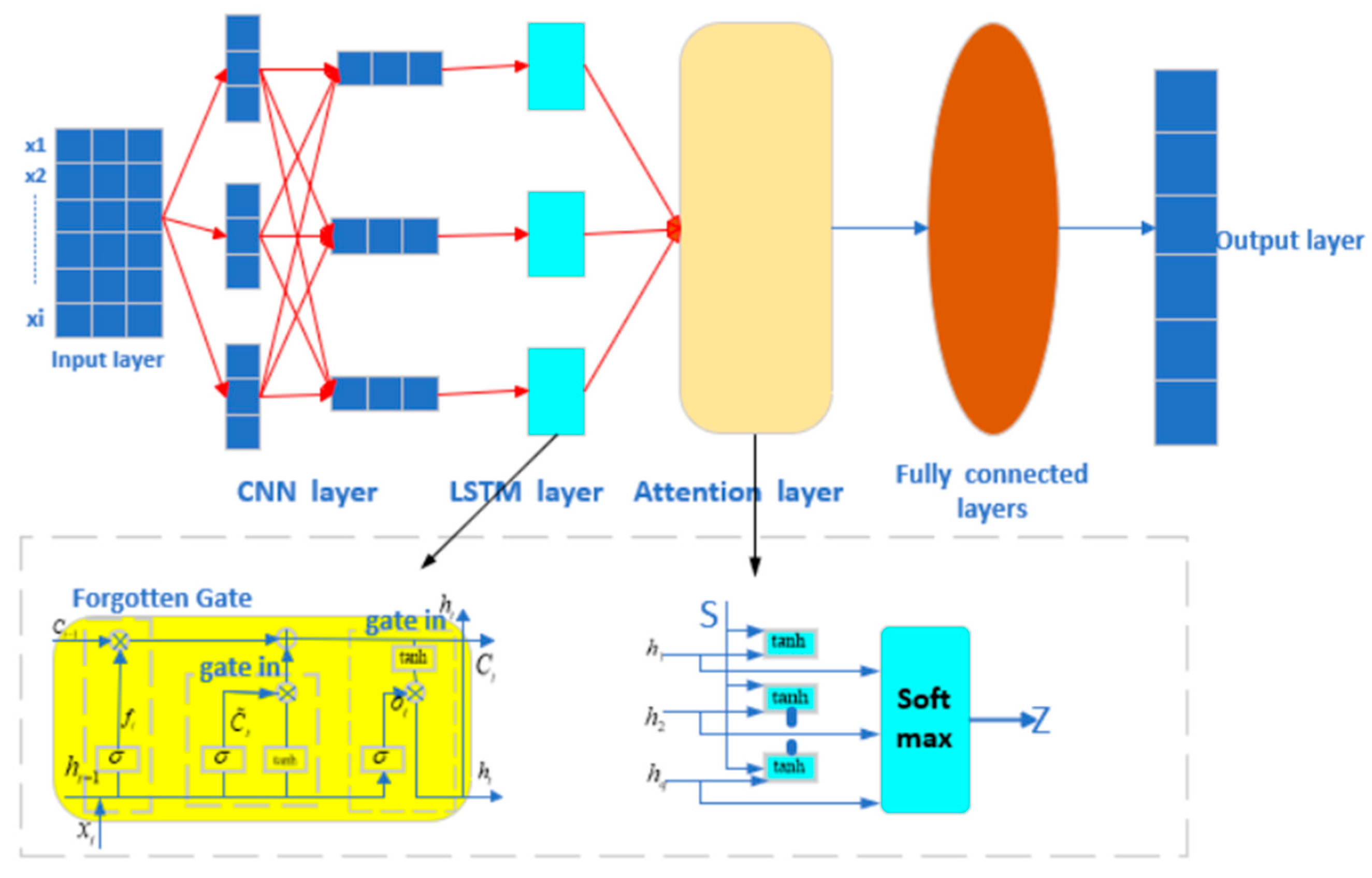
We developed a CNN-LSTM-Attention-FVIM multi-input single-output regression prediction network model that integrates CNN, LSTM, Attention, and FVIM mechanisms. The model converts the original input data into a form suitable for CNN processing. The spatial features in the data are extracted through the convolution layer. The size of the feature value is reduced through the pooling layer, and the important features are further extracted. The features extracted by the CNN are input into the LSTM network through the LSTM layer to capture the long-term dependencies in the time series data. Then, the attention mechanism is applied to the output of the LSTM through the Attention layer, the attention weight of each time step is calculated, and the weighted sum is calculated. By adjusting the key parameters such as the learning rate, hidden layer nodes, and regularization coefficient in the four-vector optimization algorithm, the model achieves the best prediction accuracy for this dataset. The main working mechanisms of the three basic models of CNN, LSTM, and Attention are as follows.
3.2. Convolutional Neural Networks
A CNN (Convolutional Neural Network) is composed of a convolution layer, activation function, pooling layer, fully connected layer, and other auxiliary layers. The function of convolution layer is to extract local features and perform dot product operation on local area with input data through sliding window (filter). The purpose of activation activation function is to introduce nonlinearity and enhance the expressiveness of the model. The role of the pooling layer is to reduce spatial dimensions, enhance translation invariance, and prevent overfitting. The functions of the fully connected layer and other auxiliary layers are to map high-level features to the sample label space (such as classification output), standardize each layer input, accelerate training, and improve generalization ability. The core of the CNN is to deconstruct spatial hierarchical feature patterns from high-dimensional data through local perception and parameter sharing. Its essence is to perform local window sliding calculation on input data through the convolution kernel (filter) to generate a feature map. By connecting convolution kernels of different sizes in parallel (such as 1 × 3, 3 × 3, 5 × 3), the CNN can capture fine-grained local features (such as instantaneous fluctuation of battery voltage) and coarse-grained global trends (such as overall capacity decay curve) at the same time. In lithium-ion battery SOH prediction, this capability enables the model to identify small distortions (early signs of degradation) and long-term trends (aging rates) in the charge and discharge curves [
35]. In traditional CNNs, the weights of each channel feature are equal, while modern variants (such as SENet) introduce channel attention mechanisms to dynamically adjust the importance of each channel. For example, in battery data, the voltage channel may be more informative than the temperature channel at a specific cycle stage, and the model can adaptively enhance the contribution of key channels.
3.3. Long Short-Term Memory Network
Long Short-Term Memory (LSTM) is a special recurrent neural network (RNN) designed to solve the problem of gradient vanishing or exploding in a traditional RNN when processing long sequence data. Its main advantages are as follows. First, LSTM effectively captures long-term dependencies in the sequence through the gating mechanism, which compensates for the problem of exponential gradient decay or explosion caused by chain derivation in traditional RNNs. Second, through the synergy of the forget gate, input gate, and output gate, LSTM dynamically controls the storage, forgetting, and output of information to avoid interference from irrelevant information. At the same time, the excellent performance in various tasks also reflects the wide applicability of the LSTM neural network model. For example, it has shown excellent predictive ability in other lithium-ion battery SOH research. Third, through the sparse activation of the gated unit, some neurons selectively participate in the calculation, creating an implicit regularization effect, which helps to alleviate overfitting. The LSTM gating mechanism includes a forget gate, input gate, update memory unit state, and output gate [
36].
- 1.
Forget gate: The main function of the forget gate is to decide which old information to discard from the cell state. The output of the forget gate is a value between 0 and 1, indicating the degree to which each piece of information is retained. The formula is as follows.
is the sigmoid activation function.
is the output of the forget gate.
is the connection between the hidden state of the previous moment and the current input.
is the weight matrix of the forget gate.
is the bias term of the forget gate.
- 2.
Input gate: The main function of the input gate is to decide what new information to store in the cell state. The sigmoid layer is used to determine the information that needs to be updated, and the tanh layer generates new candidate memory cells. The formula is as follows.
is the output of the input gate.
is the new candidate memory cell.
and are the bias term of the input gate and the candidate memory cell.
and are the weight matrix of the input gate and the candidate memory cell.
- 3.
The current memory unit is updated using the forget gate and the first two components of the input gate. The formula is as follows.
is the output of the forget gate, controlling the proportion of old memory retention,
the output of the input gate, controlling the proportion of new memory writing.
is the state of the memory unit at the current moment.
is the state of the memory unit at the previous moment.
- 4.
Output gate: The output gate controls which parts of the memory cell state will be output; that is, it determines the hidden state output at the current moment. The formula is as follows.
is the bias term of the output gate.
is the hidden state at the current moment.
is the output of the output gate.
is the weight matrix of the output gate.
The main workflow of LSTM is divided into three stages. The first is to analyze the current input xt and the previous hidden state ht−1 in the forget gate and to determine the part of the cell state that needs to be forgotten, which is the forget stage. Then, in the second stage, the memory stage, the input gate selects the key features of the input, forms candidate memories, and updates the cell state. Finally, the output gate generates the current hidden state based on the cell state updated in the previous step. This is the output stage. LSTM’s excellent ability to capture and process long-term dependencies allows it to handle complex types of sequence data, and LSTM has high flexibility. When dealing with different problems and data, it can achieve the purpose of accurate prediction by adjusting the network structure and hyperparameters.
3.4. Attention Mechanism
The core of the attention mechanism is to give the model the ability to dynamically select information so that when processing sequence data, it can independently decide which parts of the input should be focused on in the current step, rather than treating all information equally; that is, extracting the key value. First, we need to clarify a few concepts. Query is the feature representation of the current processing target (such as the hidden state of the decoder at the current moment). Key is the feature identifier of the input element, which is correlated with the query. Value is the actual content of the input element, which is weighted to generate a context vector. When receiving an input query, Attention will treat it as a query, then Attention will search for information related to the query in the given information. At this stage, it can be considered that the query is searching among many keys. After the query and a series of calculations, an output will be obtained. This involves finding the value according to the key and performing some calculation according to the value [
37]. When Attention searches for keys related to the query, it uses three weight matrices to input information to construct a multi-dimensional semantic space, and it realizes dynamic information screening through differentiated feature mapping, thereby outputting the optimal value.
is a learnable parameter for the key, used to project the key to be stored in the key space.
is a learnable parameter for query, used to project the vector to be queried into the query space.
is a learnable parameter for values, used to project the value to be stored into the value space.
is the hidden state of the encoder at time step t.
is the hidden state of the decoder at time step j.
Before obtaining the output, the query and key will be analyzed for correlation. The size of the weight is the size of the correlation value, and the correlation score is normalized by softmax:
Then, the weighted sum of the values is used to obtain the output of Attention.
where
L represents the length of the encoder input sequence, and the desired result is finally obtained. The overall process mechanism of the three models is shown in
Figure 4.
3.5. Four-Vector Optimization Algorithm
The Four-Vector Intelligent Metaheuristic (FVIM) is a new type of metaheuristic algorithm (intelligent optimization algorithm) proposed by Hussam N. Fakhouri et al. [
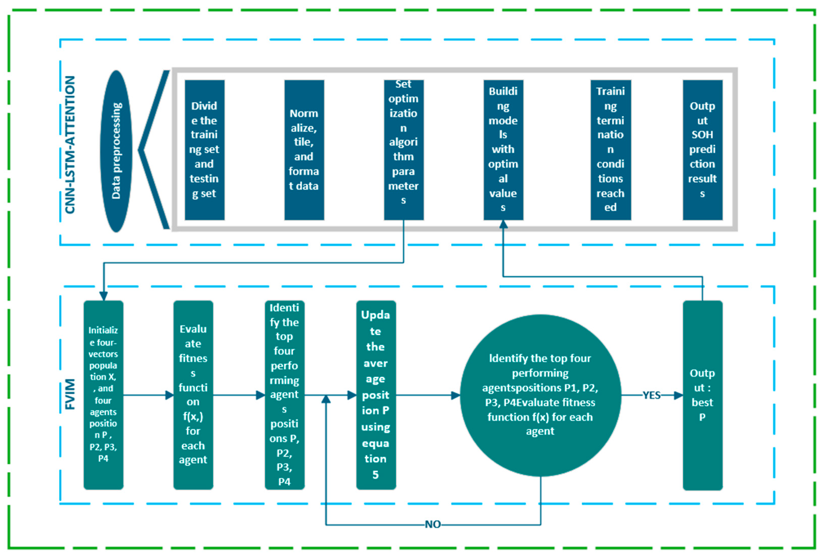
38] in 2024, which is inspired by the mathematical modeling of four vectors. The FVIM optimization process mainly consists of three stages, namely the initialization stage, the iteration stage, and the stage of finding the optimal solution. It uses the four best points in the group to determine the direction of movement of the entire group. The FVIM algorithm first identifies the four best individuals in the current group, then it calculates the average position of these four individuals to obtain a new vector position. This new position may provide a better solution for the previously determined solution, thereby guiding the group to move in a better direction. The specific stages of FVIM are as follows:
Initialize four vector populations X and four agent positions, P1, P2, P3, P4. Define and randomly initialize basic FVIM parameters. To maintain efficiency, FVIM sets upper and lower limits for each problem to limit the search space. At the same time, the number of algorithm iterations and the number of particles used by the algorithm are determined according to the complexity, size, dimension, and other characteristics of the optimization problem. Additionally, the reference fitness value is assigned 0 to assess the performance of different solutions. Certain variables are assigned extreme values to guarantee algorithm adaptability, enabling it to address both minimization and maximization objectives.
This phase is the core of FVIM, and the main steps are as follows.
Step 1: Evaluate the fitness function f(xi) for each agent,
Step 2: Identify the positions of the top four agents with the best performance, P1, P2, P3, P4,
Step 3: Update i in X(1,2,3,4) using Equations (1)–(4), and update the average position P using Equation (5), which can be described by the mathematical model as follows:
where
Xn,i represents the updated position of the nth best individual in the
i-th dimension.
Pn,i represents the current position of the nth best individual in the
i-th dimension.
Pi represents the current average position of all individuals in the
i-th dimension. α is an adaptive coefficient, which is equivalent to the search step size.
ξ1,
ξ2,
ξ3 represent random numbers uniformly distributed in the interval [0,1] [
38].
Step 4: Identify the positions of the top four agents with the best performance, P1, P2, P3, and P4, and evaluate the fitness function f(x) for each agent. If this step fails to find the best point for the four agent positions, return to step 3 and re-evaluate the fitness function f(x) for each agent. Otherwise, proceed to the next step to output the best P and end.
In the FVIM algorithm, the adaptive parameter α serves a homologous purpose to the inertia weight (W) in Particle Swarm Optimization (PSO), specifically engineered to bridge the exploration–exploitation trade-off. Exploration denotes the algorithm’s capacity to probe diverse regions for potential optima, whereas exploitation emphasizes refining search precision within promising domains to enhance solution quality. This parameter undergoes linear decay as agents approach the optimal solution. During FVIM initialization, α is strategically initialized at a substantial value of 1.5 to prioritize expansive search space exploration. Subsequently, it systematically diminishes to zero through progressive iterations as the algorithm transitions toward exploitation-dominant phases near convergence-critical regions.
The parameter is used to balance global exploration and local optimization. When is too large, the adjustment range increases, which may cause the solution to deviate from the optimal area; when is too small, it focuses on local optimization but limits the exploration ability. The specific adjustment needs to be determined according to the characteristics of the problem.
The Four-Vector Optimization Algorithm (FVIM) significantly improves the optimization performance by introducing a four-guide point strategy and a dynamic adaptive mechanism. Its core advantages include: (1) using four optimal individuals to guide the search direction, enhancing population diversity and effectively avoiding local optimal traps; (2) dynamically balancing global exploration and local development through adaptive coefficients and random perturbation parameters ξ, scanning the solution space extensively in the early stage, and focusing on fine optimization in the later stage; (3) employing a mean vector mechanism to integrate multi-guide point information and improve global convergence efficiency; (4) achieving fast convergence speed and strong robustness, especially in multimodal and high-dimensional scenarios, significantly outperforming traditional algorithms (such as PSO, GWO) and providing an efficient and reliable optimization solution for practical applications. The time series prediction model of the CNN-LSTM-Attention hybrid neural network model with FVIM added is mainly divided into the following parts: CNN-LSTM-Attention training and prediction, FVIM optimization, and various error calculations. In the initialization stage of FVIM optimization, the basic FVIM parameters are randomly initialized, and upper and lower limits are set for each problem. By setting the parameter range, randomly generating the initial population, determining the number of iterations and particle size, and assigning the baseline fitness value and extreme value variables, the algorithm is provided with a flexible search starting point to ensure that it can adapt to the optimization needs of minimization or maximization problems. In the iteration stage, the algorithm guides the movement of particles based on the dynamic motion equation and gradually converges to the global optimal solution by continuously evaluating the quality of the solution and comparing it with the objective function, finally outputing the best solution consistent with the optimization goal when the stop condition is met. The entire process aims to efficiently solve the global optimization challenges of complex problems through systematic parameter configuration and iterative optimization mechanisms while avoiding falling into local optimality.
Then, the initial parameters of the CNN-LSTM-Attention model are set, including the number of hidden layer nodes, regularization coefficients, and the selection of activation functions. This allows the neural network to have sufficient learning ability, and after finding the optimal initial parameters in the optimization algorithm, the model is constructed with the optimal weights and parameters, and then the SOH is predicted and estimated. The flowchart of the overall model is shown in
Figure 5.


 ,
, 
