Abstract
Lithium-ion batteries play a vital role in human society. Therefore, it is of critical significance to reliably predict the evolution of State of Health (SOH) degradation patterns in order to improve the high accuracy and stability of lithium-ion battery SOH prediction. This paper proposes a novel SOH predication method by combing the four-vector intelligent metaheuristic (FVIM) with the CNN-LSTM-Attention basic model. The model adopts the collaborative architecture of a convolutional neural network and time series module, strengthens the cross-level feature interaction by introducing a multi-level attention mechanism, then uses the FVIM optimization algorithm to optimize the key parameters to realize the overall model architecture. By analyzing the charging voltage curve of lithium-ion batteries, the health factors with high correlation are extracted, and the correlation between the health factors and battery capacity is verified using two correlation coefficients. After the model is verified on a single NASA battery aging dataset, the model is compared with other models under the same relevant parameters and environmental settings to verify the high-precision prediction of the model. During the analysis and comparison process, CNN-LSTM-Attention-FVIM achieved a high fitting ability for battery SOH prediction estimation, with the mean absolute error (MAE) and root mean square error (RMSE) within 0.99% and 1.33%, respectively, reflecting the model’s high generalization ability and high prediction performance.
1. Introduction
At present, the two major problems facing human society are environmental pollution and the energy crisis. As awareness grows about the severity of environmental pollution and the transformation of economic society, countries around the world are seeking clean energy such as electricity, solar energy, and wind energy to address these issues [1,2].
The most widely used clean energy at present is electricity. With the popularization of electric vehicles, mobile devices, and renewable energy storage systems, the importance of lithium-ion batteries in various fields has become increasingly prominent [3]. In the field of power batteries, lithium-ion batteries are core components of new energy vehicles, power tools, and electric bicycles, and their cost accounts for 30–40% of the total item cost [4,5]. With the continuous improvement of electric vehicle range and charging technology, higher requirements are also put forward for battery technology [6]. The battery pack of electric vehicles is composed of hundreds to thousands of single cells in series, and the SOH difference between cells can lead to a decrease in energy utilization [7]. For instance, if the capacity of a single cell degrades to 70%, the effective capacity of the entire battery pack will be limited by the “short board effect”, resulting in energy waste [8]. At the same time, for end users, overcharging, over-discharging, or local overheating of the battery may cause thermal runaway, or even fire and explosion. As the battery ages, capacity decay will also cause a significant decrease in vehicle range. SOH prediction is not only a technical indicator of battery management but also a core link between safety, economy, and environmental protection. Real-time and accurate prediction of battery SOH is essential [9].
Battery health state (SOH) is a core indicator for measuring battery performance degradation, usually defined as the ratio of the current maximum capacity or internal resistance to the initial value [10]. At present, SOH estimation methods can be divided into model-based methods and data-driven methods, which have significant differences in principles, implementation, and applicable scenarios [11]. First, the model-based method describes the internal dynamic process of the battery by establishing physical or electrochemical equations, and it uses the difference between observable external parameters (such as voltage, current, temperature) and model output to estimate the state. Its core is to associate the microscopic aging mechanism of the battery with the macroscopic behavior through mathematical modeling. There are two typical models: the electrochemical model and the equivalent circuit model. The principle of the electrochemical model is based on porous electrode theory (Pseudo-Two-Dimensional, P2D model), which describes the diffusion, insertion, or extraction process of lithium ions in positive and negative electrode materials by coupling mass conservation, charge conservation, and reaction kinetics equations [12]. Its advantage lies in accurately characterizing the internal aging mechanism of the battery (such as SEI film growth and active material loss), which is suitable for mechanism research. However, the model has several disadvantages, including high model complexity (requiring the solution of high-dimensional partial differential equations), time-consuming calculations (with a single simulation taking several hours); difficulty in parameter identification (e.g., diffusion coefficients and reaction rate constants); and challenges in real-time online application. The principle of the equivalent circuit model is to use circuit elements such as resistors and capacitors to simulate the dynamic response of the battery [13]. Common models usually include the following: (1) Rint model: only contains ohmic internal resistance; (2) Thevenin model: series RC network simulates polarization effect; (3) Dual Polarization (DP) model: dual RC network distinguishes between fast and slow polarization processes. The advantages and disadvantages of this model are also obvious. The advantage is that the calculation is simple (high real-time performance) and suitable for BMS online estimation [14]. One disadvantage is that it cannot describe the internal aging mechanism of the battery and can only reflect the changes in macroscopic parameters. In order to solve the problem of inconsistency of electrochemical parameters caused by differences in battery manufacturing, Zhang et al. [15] characterized individual differences through initial cycle state data and constructed a physical information dual neural network (PIDNN) to achieve dual functions: dynamic estimation of electrochemical parameters (such as lithium ion diffusion coefficient, reaction rate constant, etc.) and synchronous simulation of lithium ion concentration distribution in solid electrodes and electrolytes. The electrochemical model based on physical principles is combined with the deep learning model to break through the limitations of traditional data-driven methods that lack physical interpretability. It provides a new paradigm for SOH estimation with few samples, high precision, and clear interpretability. Liu et al. [16] designed the battery physical information neural network (BatteryPINN) based on the mathematical model of solid electrolyte interface (SEI) film growth, and they embedded physical laws such as SEI film thickness evolution into the network structure. By explicitly modeling the SEI film growth process, the quantitative relationship between capacity decay and SEI film thickness is revealed, providing physical insights into the prediction results and overcoming the limitations of the “black box model”. In addition, the improved composite multi-scale Hilbert cumulative residual entropy algorithm is used to automatically extract high-quality health features directly from battery voltage and current data, providing a new idea for accurate, interpretable, and easy-to-deploy battery SOH estimation. Tran et al. [17] continuously monitored Thevenin ECM (equivalent circuit model) parameters through cycle aging experiments and quantified their evolution with SOH degradation. After integrating the SOH factor, the voltage prediction error of the Thevenin model on the aged battery was reduced by about 40%, and the average accuracy of the whole life cycle was more than 99%. The system revealed the quantitative influence of SOH on Thevenin ECM parameters and realized the efficient prediction of ECM parameters under the synergy of multiple factors. It provided a core algorithm for adaptive ECM parameter update for smart BMS. Li et al. [18] constructed an enhanced equivalent circuit model (ECMC) by adding capacitor elements to the classic ECM to improve the fitting ability of full-band EIS data. Optimization algorithms such as the nonlinear least squares method were used to identify ECMC model parameters and capture the evolution of parameters with battery aging. This provides a high-precision and highly adaptable SOH estimation scheme for BMS, particularly for actual working conditions under severe temperature fluctuations.
Compared with the above methods, the data-driven method analyzes the characteristics of battery aging cycle data in a simple way and establishes a relationship model between battery characteristics and SOH [19]. The principle of the data-driven method is that the data-driven method abandons physical modeling and directly mines the statistical association between battery aging characteristics and SOH from historical data. The nonlinear mapping relationship between input (health features) and output (SOH) is constructed through machine learning algorithms [20,21]. The core steps of this data-driven model are health feature (HF) extraction, typical algorithm selection, and model training and verification. Among them, common traditional machine learning includes support vector regression (SVR): mapping high-dimensional space through kernel functions (such as RBF) to construct regression hyperplanes; random forests: integrating multiple decision trees to reduce the risk of overfitting. Deep learning includes long short-term memory networks (LSTM): capturing the temporal dependence of capacity decay; convolutional neural networks (CNNs): extracting local aging features from charge and discharge curve images [22,23,24,25]. The above models have the advantages of not requiring prior physical knowledge, adapting to complex nonlinear relationships, and being able to integrate multi-source data (such as temperature, current, and voltage series) [26]. However, they rely on a large amount of labeled data (complete aging cycle data is required); the model has poor interpretability (the “black box” feature limits engineering trust); and the generalization ability for unseen working conditions (such as extreme temperature and fast charging strategy) is insufficient [27]. Xu et al. [28] proposed a CNN-LSTM-Skip hybrid model. The CNN extracts local time series features, LSTM captures long-term dependencies, and skip connections achieve cross-layer feature complementarity, enhancing the model’s ability to characterize battery aging patterns. The method was verified on a public dataset, covering different battery types, charging and discharging conditions, and aging trajectories. It provides an efficient, robust, and scalable SOH estimation solution for battery health management. Sun et al. [29] used CNN-LSTM-Attention tri-modal fusion to extract the local spatiotemporal features of the battery capacity/voltage curve (such as charging and discharging platform fluctuations); the LSTM layer captured the long-term sequence dependencies of capacity decay, and the attention mechanism dynamically focused on key degradation stages (such as capacity inflection points and mutation intervals). Through attention weight allocation, the model’s sensitivity to capacity regeneration phenomena was enhanced, and noise interference was suppressed. This approach improves the ability to characterize nonlinear degradation trajectories, providing a highly robust and generalizable prediction scheme for achieving more accurate SOH prediction and estimation of batteries.
Combining the advantages and disadvantages of the above models, this paper focuses on analyzing and studying the key challenges in health feature construction and algorithms in response to the insufficient research on existing lithium-ion battery aging prediction trajectories. This paper innovatively adds the four-vector (FVIM) optimization algorithm to CNN-LSTM-Attention and integrates multiple health factors to predict and estimate battery SOH. First, HFs with high correlation with SOH are extracted from the battery charging cycle, then the Pearson and Spearman correlation coefficients are used to evaluate the correlation between health factors and SOH. Next, a data-driven model is constructed, and the model parameters are optimized using the four-vector optimization algorithm. Subsequently some key network layers are fine-tuned to adapt to the dataset used. The prediction results are then compared with other deep learning methods to verify the superiority and applicability of this study.
2. Lithium-Ion Battery Data Explanation and Health Factor Selection
2.1. Battery Data Description
This paper uses the well-known NASA lithium-ion battery dataset as the research object, in which the battery model is the 18,650 lithium iron phosphate battery. The following experimental operations are performed on B0005, B0006, B0007, and B0018 batteries at a battery experimental temperature of 24 °C and a rated capacity of 2 Ah. The first step is to charge the four batteries with constant current and constant voltage. Under the current environmental conditions, they are first charged with a constant current of 1.5 A. When the battery voltage reaches 4.2 V, they are charged with constant voltage and current. When the current reaches 20 mA, the first step ends; that is, the charging stage ends. The second step is to discharge the battery with a constant current of 2 A and discharge B0005, B0006, B0007, and B0018 to cut-off voltages of 2.7 V, 2.5 V, 2.2 V, and 2.5 V, respectively [30]. At this point, a charge and discharge experiment is completed. Then, in order to accelerate battery aging, the above operation is repeated. When the actual capacity of each battery is less than 1.4 Ah, the end-of-life condition is reached. The capacity degradation curves generated by the four batteries are shown in Figure 1. The corresponding parameters are shown in Table 1.
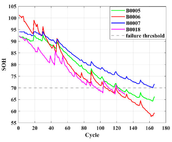
Figure 1.
Capacity degradation curve.

Table 1.
Relevant battery parameters.
2.2. Selection of Health Factors
Since SOH cannot be measured directly, and the raw data of the battery such as voltage and current are generated during the battery charging and discharging process, but they will be affected by the operation of the battery itself, causing these data to be disturbed. Therefore, using them to predict battery SOH is not accurate. In contrast, HF (health factor) is extracted from these voltage and current data [31]. By properly selecting HF as the model input, the above-mentioned interference factors can be effectively weakened or eliminated, and the inherent characteristics and changing trends of the battery can be more realistically revealed, thereby improving the reliability and accuracy of the prediction.
In practice, lithium-ion batteries are more stable when charging than when discharging. To this end, the current–time curve, voltage–time curve, and temperature–time curve of the B0005 battery under different cycles of charging and discharging are compared, as shown in Figure 2a–f. To clearly illustrate the state of charge and discharge of each battery over time, the curves in the figure are presented in a gradual gradient from light to dark. The charging process of lithium-ion batteries is generally divided into a constant current charging stage (CC) and a constant voltage charging stage (CV). The battery is charged with constant current to the voltage charging limit, then it enters constant voltage charging to maintain a constant charging current. The charging time of the battery is essentially determined by the available capacity. When the battery health state (SOH) decreases, the reduction in its actual available capacity will directly shorten the duration of the constant current charging stage. It is worth noting that in the case of capacity decay, in order to achieve a fully charged state, the subsequent constant voltage charging stage may require additional extended operation time. As shown in Figure 2a–f, the constant current charging time of the battery and the time when the cut-off voltage and temperature reach the peak value show a trend of gradually shortening when charging under different cycle periods, and the time when the charging temperature reaches the peak value is gradually advanced, showing a certain regularity and stability. At the same time, the current–time, voltage–time, and temperature–time curves during discharge are affected by various factors and have poor stability [32]. Taking all factors into consideration, we selected five health factors, namely equal pressure rise charging time, constant current charging time, constant voltage charging time, corresponding time of temperature peak during charging, and constant current charging time ratio, as the characteristics of this SOH characterization. In addition, the above five health factors are marked as HF1, HF2, HF3, HF4, and HF5 in order to facilitate subsequent research and description.
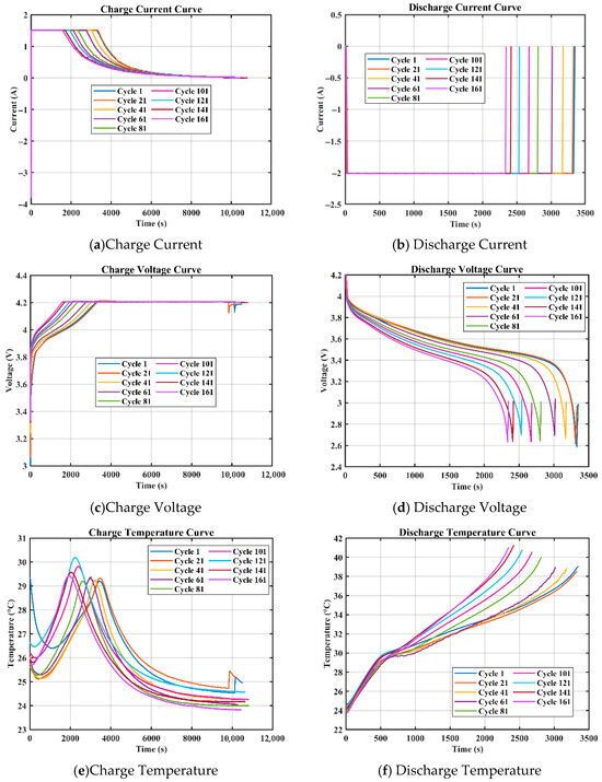
Figure 2.
Battery charge and discharge status.
In this study, we extracted five health factors (HFS) of the B0005 battery, and in order to make the data distribution more reasonable, improve the robustness of the algorithm, and accelerate convergence, we normalized it. As shown in Figure 3, there is information overlap in the five extracted health factors [33,34]. It can be seen that in order to reduce the computing cost, normalization is necessary.
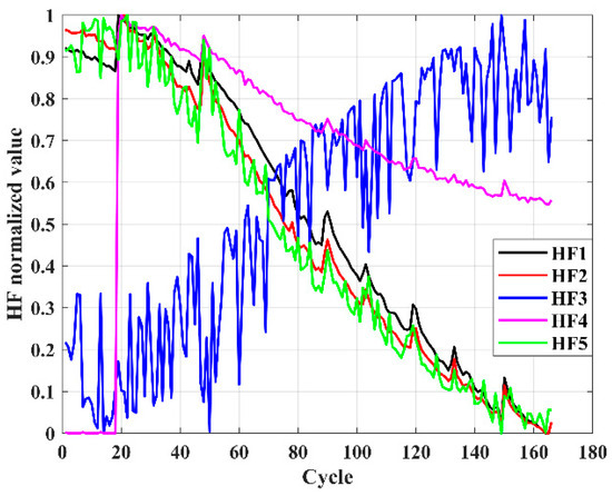
Figure 3.
Health factor curves of B0005 battery.
2.3. Correlation Between Health Factor and Battery SOH
In order to verify whether there was a correlation between HFS and SOH, we used Pearson and Spearman correlation coefficients as evaluation criteria. The main difference between the two is that Pearson focuses on linearity, while Spearman focuses on monotony. The former requires continuity and a normal distribution, while the latter has low requirements for data and can be ordered. Pearson may be more sensitive to outliers, while Spearman has less influence because of the use of ranks. The value range of the Pearson correlation and Spearman correlation coefficients is between −1 and 1. The closer the absolute value is to 1, the higher the correlation between the variables. If the value is close to 0, it indicates that the linear correlation is weak. Using two correlation coefficients simultaneously can make the correlation results more convincing. The following is the specific calculation formula.
Here, X and Y represent the entire sample, and xi and yi represent individuals in the sample. It can be seen from Table 2 that, except for the low correlation of the constant voltage charging time of the B0018 battery, the other five HFS used have a high correlation with SOH, which is above 0.9 or near 0.9, and its HFS has a good representation of the SOH. Therefore, when predicting and estimating the B0018 battery, we exclude the HF3 constant voltage charging time of the B0018 battery and only use the other four health factors with the higher correlation.
Table 2.
Results of HFS and SOH correlation index.
3. Algorithm Principle Explanation
3.1. Explanation of Basic Models: CNN, LSTM, and Attention
We developed a CNN-LSTM-Attention-FVIM multi-input single-output regression prediction network model that integrates CNN, LSTM, Attention, and FVIM mechanisms. The model converts the original input data into a form suitable for CNN processing. The spatial features in the data are extracted through the convolution layer. The size of the feature value is reduced through the pooling layer, and the important features are further extracted. The features extracted by the CNN are input into the LSTM network through the LSTM layer to capture the long-term dependencies in the time series data. Then, the attention mechanism is applied to the output of the LSTM through the Attention layer, the attention weight of each time step is calculated, and the weighted sum is calculated. By adjusting the key parameters such as the learning rate, hidden layer nodes, and regularization coefficient in the four-vector optimization algorithm, the model achieves the best prediction accuracy for this dataset. The main working mechanisms of the three basic models of CNN, LSTM, and Attention are as follows.
3.2. Convolutional Neural Networks
A CNN (Convolutional Neural Network) is composed of a convolution layer, activation function, pooling layer, fully connected layer, and other auxiliary layers. The function of convolution layer is to extract local features and perform dot product operation on local area with input data through sliding window (filter). The purpose of activation activation function is to introduce nonlinearity and enhance the expressiveness of the model. The role of the pooling layer is to reduce spatial dimensions, enhance translation invariance, and prevent overfitting. The functions of the fully connected layer and other auxiliary layers are to map high-level features to the sample label space (such as classification output), standardize each layer input, accelerate training, and improve generalization ability. The core of the CNN is to deconstruct spatial hierarchical feature patterns from high-dimensional data through local perception and parameter sharing. Its essence is to perform local window sliding calculation on input data through the convolution kernel (filter) to generate a feature map. By connecting convolution kernels of different sizes in parallel (such as 1 × 3, 3 × 3, 5 × 3), the CNN can capture fine-grained local features (such as instantaneous fluctuation of battery voltage) and coarse-grained global trends (such as overall capacity decay curve) at the same time. In lithium-ion battery SOH prediction, this capability enables the model to identify small distortions (early signs of degradation) and long-term trends (aging rates) in the charge and discharge curves [35]. In traditional CNNs, the weights of each channel feature are equal, while modern variants (such as SENet) introduce channel attention mechanisms to dynamically adjust the importance of each channel. For example, in battery data, the voltage channel may be more informative than the temperature channel at a specific cycle stage, and the model can adaptively enhance the contribution of key channels.
3.3. Long Short-Term Memory Network
Long Short-Term Memory (LSTM) is a special recurrent neural network (RNN) designed to solve the problem of gradient vanishing or exploding in a traditional RNN when processing long sequence data. Its main advantages are as follows. First, LSTM effectively captures long-term dependencies in the sequence through the gating mechanism, which compensates for the problem of exponential gradient decay or explosion caused by chain derivation in traditional RNNs. Second, through the synergy of the forget gate, input gate, and output gate, LSTM dynamically controls the storage, forgetting, and output of information to avoid interference from irrelevant information. At the same time, the excellent performance in various tasks also reflects the wide applicability of the LSTM neural network model. For example, it has shown excellent predictive ability in other lithium-ion battery SOH research. Third, through the sparse activation of the gated unit, some neurons selectively participate in the calculation, creating an implicit regularization effect, which helps to alleviate overfitting. The LSTM gating mechanism includes a forget gate, input gate, update memory unit state, and output gate [36].
- 1.
- Forget gate: The main function of the forget gate is to decide which old information to discard from the cell state. The output of the forget gate is a value between 0 and 1, indicating the degree to which each piece of information is retained. The formula is as follows.
is the sigmoid activation function.
is the output of the forget gate.
is the connection between the hidden state of the previous moment and the current input.
is the weight matrix of the forget gate.
is the bias term of the forget gate.
- 2.
- Input gate: The main function of the input gate is to decide what new information to store in the cell state. The sigmoid layer is used to determine the information that needs to be updated, and the tanh layer generates new candidate memory cells. The formula is as follows.
is the output of the input gate.
is the new candidate memory cell.
and are the bias term of the input gate and the candidate memory cell.
and are the weight matrix of the input gate and the candidate memory cell.
- 3.
- The current memory unit is updated using the forget gate and the first two components of the input gate. The formula is as follows.
is the output of the forget gate, controlling the proportion of old memory retention,
the output of the input gate, controlling the proportion of new memory writing.
is the state of the memory unit at the current moment.
is the state of the memory unit at the previous moment.
- 4.
- Output gate: The output gate controls which parts of the memory cell state will be output; that is, it determines the hidden state output at the current moment. The formula is as follows.
is the bias term of the output gate.
is the hidden state at the current moment.
is the output of the output gate.
is the weight matrix of the output gate.
The main workflow of LSTM is divided into three stages. The first is to analyze the current input xt and the previous hidden state ht−1 in the forget gate and to determine the part of the cell state that needs to be forgotten, which is the forget stage. Then, in the second stage, the memory stage, the input gate selects the key features of the input, forms candidate memories, and updates the cell state. Finally, the output gate generates the current hidden state based on the cell state updated in the previous step. This is the output stage. LSTM’s excellent ability to capture and process long-term dependencies allows it to handle complex types of sequence data, and LSTM has high flexibility. When dealing with different problems and data, it can achieve the purpose of accurate prediction by adjusting the network structure and hyperparameters.
3.4. Attention Mechanism
The core of the attention mechanism is to give the model the ability to dynamically select information so that when processing sequence data, it can independently decide which parts of the input should be focused on in the current step, rather than treating all information equally; that is, extracting the key value. First, we need to clarify a few concepts. Query is the feature representation of the current processing target (such as the hidden state of the decoder at the current moment). Key is the feature identifier of the input element, which is correlated with the query. Value is the actual content of the input element, which is weighted to generate a context vector. When receiving an input query, Attention will treat it as a query, then Attention will search for information related to the query in the given information. At this stage, it can be considered that the query is searching among many keys. After the query and a series of calculations, an output will be obtained. This involves finding the value according to the key and performing some calculation according to the value [37]. When Attention searches for keys related to the query, it uses three weight matrices to input information to construct a multi-dimensional semantic space, and it realizes dynamic information screening through differentiated feature mapping, thereby outputting the optimal value.
is a learnable parameter for the key, used to project the key to be stored in the key space.
is a learnable parameter for query, used to project the vector to be queried into the query space.
is a learnable parameter for values, used to project the value to be stored into the value space.
is the hidden state of the encoder at time step t.
is the hidden state of the decoder at time step j.
Before obtaining the output, the query and key will be analyzed for correlation. The size of the weight is the size of the correlation value, and the correlation score is normalized by softmax:
Then, the weighted sum of the values is used to obtain the output of Attention.
where L represents the length of the encoder input sequence, and the desired result is finally obtained. The overall process mechanism of the three models is shown in Figure 4.
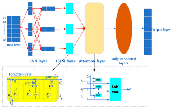
Figure 4.
CNN-LSTM-Attention model flow chart.
3.5. Four-Vector Optimization Algorithm
The Four-Vector Intelligent Metaheuristic (FVIM) is a new type of metaheuristic algorithm (intelligent optimization algorithm) proposed by Hussam N. Fakhouri et al. [38] in 2024, which is inspired by the mathematical modeling of four vectors. The FVIM optimization process mainly consists of three stages, namely the initialization stage, the iteration stage, and the stage of finding the optimal solution. It uses the four best points in the group to determine the direction of movement of the entire group. The FVIM algorithm first identifies the four best individuals in the current group, then it calculates the average position of these four individuals to obtain a new vector position. This new position may provide a better solution for the previously determined solution, thereby guiding the group to move in a better direction. The specific stages of FVIM are as follows:
- Phase 1. Initialization phase
Initialize four vector populations X and four agent positions, P1, P2, P3, P4. Define and randomly initialize basic FVIM parameters. To maintain efficiency, FVIM sets upper and lower limits for each problem to limit the search space. At the same time, the number of algorithm iterations and the number of particles used by the algorithm are determined according to the complexity, size, dimension, and other characteristics of the optimization problem. Additionally, the reference fitness value is assigned 0 to assess the performance of different solutions. Certain variables are assigned extreme values to guarantee algorithm adaptability, enabling it to address both minimization and maximization objectives.
- Phase 2. Iteration phase
This phase is the core of FVIM, and the main steps are as follows.
Step 1: Evaluate the fitness function f(xi) for each agent,
Step 2: Identify the positions of the top four agents with the best performance, P1, P2, P3, P4,
Step 3: Update i in X(1,2,3,4) using Equations (1)–(4), and update the average position P using Equation (5), which can be described by the mathematical model as follows:
where Xn,i represents the updated position of the nth best individual in the i-th dimension. Pn,i represents the current position of the nth best individual in the i-th dimension. Pi represents the current average position of all individuals in the i-th dimension. α is an adaptive coefficient, which is equivalent to the search step size. ξ1, ξ2, ξ3 represent random numbers uniformly distributed in the interval [0,1] [38].
Step 4: Identify the positions of the top four agents with the best performance, P1, P2, P3, and P4, and evaluate the fitness function f(x) for each agent. If this step fails to find the best point for the four agent positions, return to step 3 and re-evaluate the fitness function f(x) for each agent. Otherwise, proceed to the next step to output the best P and end.
In the FVIM algorithm, the adaptive parameter α serves a homologous purpose to the inertia weight (W) in Particle Swarm Optimization (PSO), specifically engineered to bridge the exploration–exploitation trade-off. Exploration denotes the algorithm’s capacity to probe diverse regions for potential optima, whereas exploitation emphasizes refining search precision within promising domains to enhance solution quality. This parameter undergoes linear decay as agents approach the optimal solution. During FVIM initialization, α is strategically initialized at a substantial value of 1.5 to prioritize expansive search space exploration. Subsequently, it systematically diminishes to zero through progressive iterations as the algorithm transitions toward exploitation-dominant phases near convergence-critical regions.
The parameter is used to balance global exploration and local optimization. When is too large, the adjustment range increases, which may cause the solution to deviate from the optimal area; when is too small, it focuses on local optimization but limits the exploration ability. The specific adjustment needs to be determined according to the characteristics of the problem.
The Four-Vector Optimization Algorithm (FVIM) significantly improves the optimization performance by introducing a four-guide point strategy and a dynamic adaptive mechanism. Its core advantages include: (1) using four optimal individuals to guide the search direction, enhancing population diversity and effectively avoiding local optimal traps; (2) dynamically balancing global exploration and local development through adaptive coefficients and random perturbation parameters ξ, scanning the solution space extensively in the early stage, and focusing on fine optimization in the later stage; (3) employing a mean vector mechanism to integrate multi-guide point information and improve global convergence efficiency; (4) achieving fast convergence speed and strong robustness, especially in multimodal and high-dimensional scenarios, significantly outperforming traditional algorithms (such as PSO, GWO) and providing an efficient and reliable optimization solution for practical applications. The time series prediction model of the CNN-LSTM-Attention hybrid neural network model with FVIM added is mainly divided into the following parts: CNN-LSTM-Attention training and prediction, FVIM optimization, and various error calculations. In the initialization stage of FVIM optimization, the basic FVIM parameters are randomly initialized, and upper and lower limits are set for each problem. By setting the parameter range, randomly generating the initial population, determining the number of iterations and particle size, and assigning the baseline fitness value and extreme value variables, the algorithm is provided with a flexible search starting point to ensure that it can adapt to the optimization needs of minimization or maximization problems. In the iteration stage, the algorithm guides the movement of particles based on the dynamic motion equation and gradually converges to the global optimal solution by continuously evaluating the quality of the solution and comparing it with the objective function, finally outputing the best solution consistent with the optimization goal when the stop condition is met. The entire process aims to efficiently solve the global optimization challenges of complex problems through systematic parameter configuration and iterative optimization mechanisms while avoiding falling into local optimality.
Then, the initial parameters of the CNN-LSTM-Attention model are set, including the number of hidden layer nodes, regularization coefficients, and the selection of activation functions. This allows the neural network to have sufficient learning ability, and after finding the optimal initial parameters in the optimization algorithm, the model is constructed with the optimal weights and parameters, and then the SOH is predicted and estimated. The flowchart of the overall model is shown in Figure 5.
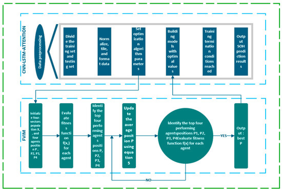
Figure 5.
Overall model flowchart.
4. Model Evaluation Criteria
The general evaluation indicators include MAE, RMSE, MBE, MAPE, MSE, etc. Combined with the prediction characteristics of this model, we use the mean absolute error (MAE) and root mean square error (RMSE) to evaluate the feasibility of the proposed method. The lower the values of MAE and RMSE, the higher the accuracy of the proposed model prediction method. The relevant calculation formula is as follows.
5. Verify the Feasibility of the Model and Analyze the Relevant Results
5.1. Description of Results Related to a Single Dataset
After completing the above preparations, the processed dataset is input into the CNN-LSTM-Attention-FVIM prediction model. In this part, we use the battery aging data of B0005, B0007, and B0018 for prediction, and we train 60% and 50% of the battery data before predicting the battery life to achieve multi-faceted evaluation of the model. First, Figure 6a–c represent the prediction graphs of 50% of the training data of the three batteries, B0005, B0007, and B0018, Figure 7a–c represent the prediction graphs of 60% of the training data of the three batteries, Figure 6d–f represent the error graphs of 50% of the training data of the three batteries, and Figure 7d–f represent the error graphs of 60% of the training data of the three batteries. First, it can be seen from the prediction graphs for 50% and 60% of the training data that the model has good prediction ability and can accurately fit the capacity decay trajectory of the B0005, B0007, and B0018 batteries. Regardless of the number of training samples, the prediction curve is still highly consistent with the true value. The CNN-LSTM-Attention-FVIM regression prediction model can effectively capture the battery aging characteristics and stabilize the prediction accuracy within a certain range through adaptive functions and dynamic adjustment of key parameters. In addition, to show the size of the prediction error of this model more intuitively, compass charts are used to characterize other performance indicators such as MAE and RMSE. As shown in Figure 6d–f and Figure 7d–f, the test set axes of the two graphs of RMSE and MAE are close to the center, forming a small circle. In addition, the axis lengths of MAE and RMSE of a single battery are close, indicating that the error distribution is uniform and there is no large outlier error. At the same time, it can be clearly seen from the data shown in the figure that MAE and RMSE are around 1%. The error is stable without obvious fluctuations. At the same time, in order to more intuitively show the model’s ability to fit the data, we selected the B0018 battery with relatively large error and showed its data fitting graph and relative error graph, as shown in Figure 8a,b. From the two figures, it can be clearly seen that most of the data are near the baseline, and the relative error distribution is concentrated, mostly distributed around 0.01 to −0.01, indicating that the model is robust. At the same time, from the data in Table 3, it can be intuitively seen that the MAE and RMSE of the proposed model are significantly better than other models. Among them, the range of MAE of this model is stable at about 0.7%, and the range of RMSE is stable at around 1%. Compared with other models, the CNN-LSTM-Attention-FVIM prediction model has good adaptability and robustness for the three groups of batteries, which also proves that the model proposed in this paper has good estimation ability in the face of SOH changes. From Table 4, it can be seen that when the proportion of the training set increases to 60%, the MAE and RMSE of the three groups of batteries are still small, and the prediction accuracy is still high, proving that the model has excellent degradation feature learning ability.
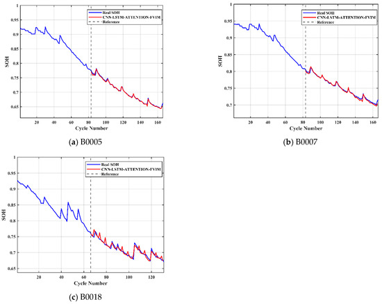
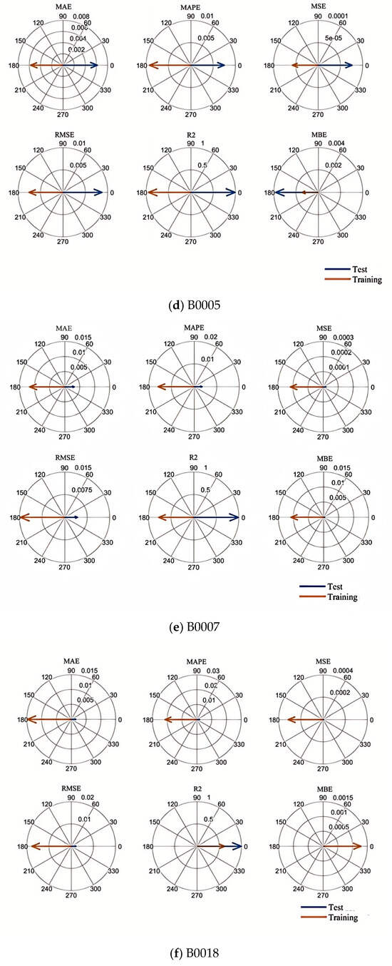
Figure 6.
Prediction graph and error graph of each battery when the training data is 50%.
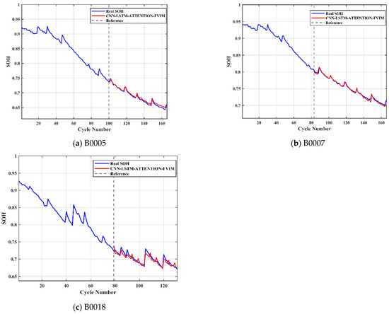
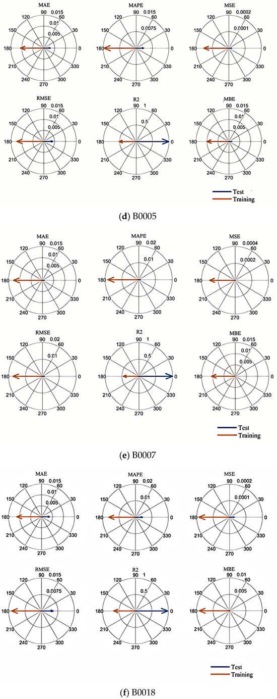
Figure 7.
Prediction graph and error graph of each battery when the training data is 60%.
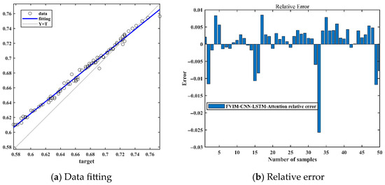
Figure 8.
Fitting diagram and relative error diagram of B0018 battery.
Table 3.
Results of various evaluation indicators when the training data is 50%.
Table 4.
Results of various evaluation indicators when the training data is 60%.
These experimental results fully verify the outstanding performance and stability of the CNN-LSTM-Attention-FVIM model in SOH prediction. The prediction model proposed in this study can accurately estimate and predict the SOH of batteries across varying training sample sizes, owing to its effective extraction and learning of battery degradation characteristics, while maintaining prediction accuracy unaffected by sample quantity constraints.
5.2. Comparison and Verification of Different Models
In order to verify the stability and excellence of this model and to better interpret the characteristics of this model, we used the processed NASA battery data to predict and estimate using other GRU models, BILSTM models, CNN models, and CNN-LSTM-Attention models. These results were then compared and verified with the CNN-LSTM-Attention-FVIM optimization prediction model proposed in this paper. For this comparison and verification, we used B0005, B0006, B0007, and B0018 batteries from NASA. Under the same conditions as the other parameters, we used 70% of the battery data as the training set for each model and the remaining 30% as the test set for estimation and comparison. The SOH prediction comparison chart of each model is shown in Figure 9a–d, and a comparison of the MAE and RMSE indicators for each model is shown in Figure 10.
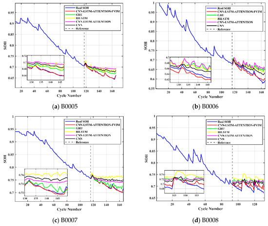
Figure 9.
Comparison of prediction effects of different models.
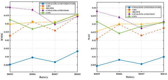
Figure 10.
Comparison of evaluation indicators of different models.
From Figure 9, the model SOH prediction estimation comparison chart shows that CNN-LSTM-Attention-FVIM has a strong prediction ability for experimental battery data, especially for the B0005 battery and B0007 battery. The prediction curve and the true curve are almost completely overlapping, demonstrating the superiority of the CNN-LSTM-Attention-FVIM model prediction. In contrast, the prediction accuracy of the GRU model, BILSTM model, CNN model, and CNN-LSTM-Attention model is poor. Their prediction curves are mostly above the true value, and the curve following is also poor, with large fluctuations resulting in large amplitudes and poor stability. However, CNN-LSTM-Attention-FVIM has multiple performances that are significantly better than other models. In addition, it also shows excellent fitting in the battery capacity regeneration stage, meaning it still has good predictability for battery SOH, showing good robustness and stability, providing a new solution for battery SOH prediction.
The RMSE and MAE Index data of different datasets and different prediction models are shown in Table 5. It can be seen from Table 5 that the prediction accuracy of the single CNN model and the CNN-LSTM-Attention model is poor, and the error is large. The maximum MAE and RMSE of the two models reached 3.78% and 3.98%, respectively. At the same time, the GRU model and the BILSTM model are still not ideal for the prediction of battery SOH. With the increase in battery aging times, the linearity of the aging curve becomes weaker, and the deviation between the prediction result and the actual value increases in the later period. The RMSE and MAE of the CNN-LSTM-Attention-FVIM model we developed are 1.33% and 0.99% at the maximum. Among them, the evaluation index MAE of the B0018 battery is 64%, 68.27%, 67.96%, and 68.47% lower than that of the GRU model, BILSTM model, CNN model, and CNN-LSTM-Attention model, respectively. It can be seen that the CNN-LSTM-Attention-FVIM model performs well in most cases and has better stability. This also shows that the model proposed in this paper is more feasible for the prediction and estimation of lithium-ion battery SOH.
Table 5.
Evaluation index data of different models.
The above results show the predicted effects of multiple batteries, but batteries B0006 and B0018 are slightly inferior to the other two, which may be related to the following situations. First, CNN has two characteristics: translation invariance and local feature extraction. It captures the local morphological features of the charge and discharge curves (such as voltage platform fluctuations) to adapt to charging segments with different starting points, thereby achieving the predictive advantage of identifying early degradation features (such as shortening the constant current stage). LSTM stores long-term attenuation trends through a gating mechanism to capture capacity regeneration phenomena. Attention focuses on key stages, enhances the weight and noise suppression of degradation inflection points (such as capacity mutation cycles), and reduces the impact of non-critical cycles (such as the late stage of constant voltage charging), thereby reducing the errors caused by random charging fluctuations. The FVIM optimization algorithm improves the prediction performance of the model by optimizing key parameters such as the learning rate and regularization coefficient. The combination of these four models achieves accurate prediction of the dataset. The prediction error indicators of the B0006 and B0018 batteries are larger than those of the B0005 and B0007 batteries. This is due to the following reasons. First, based on existing deep learning-related research, due to the data characteristics contained in the B0006 battery dataset itself, the prediction accuracy is inferior to other datasets. Secondly, the deep learning model also has certain uncertainties. The prediction method of each model is different, resulting in prediction differences between similar models. This also causes the prediction error of the B0018 battery dataset to be inferior to that of the B0005 and B0007 datasets. At the same time, the high error of the B0018 battery may be related to data fluctuations or degradation characteristics, which affect the model fitting ability. But overall, the model proposed in this paper is still more competitive and stable than the other similar models. Second, we found that in other related studies, the B0006 and B0018 battery datasets were inferior to the B0005 and B0007 battery datasets.
5.3. University of Maryland Dataset Validation
The above description uses four battery datasets provided by NASA to verify the CNN-LSTM-Attention-FVIM model in this paper, which reflects the strong predictive ability of the model proposed in this paper. In order to further verify the generalization ability and robustness of the model, we used the CS2-35 and CS2-37 battery datasets provided by the University of Maryland for prediction and verification. We did not modify any parameters, we used the same health features as the NASA dataset, and we provided 70% of the data as the training set for predicting and estimating. As shown in Figure 11, the CNN-LSTM-Attention-FVIM model proposed in this paper still has a high predictive ability, and the predicted value is very consistent with the true value. This shows that the model proposed in this paper has a strong generalization ability, and it can have a strong predictive estimation ability in the face of datasets from different sources, showing adaptability to the downward trend of different datasets.
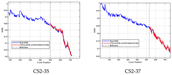
Figure 11.
University of Maryland single dataset.
In order to more intuitively show the prediction ability of the model for the University of Maryland dataset, we still use RMSE and MAE as evaluation indicators. The specific values are shown in Table 6. As can be seen from the table, both error indicators are no more than 0.87%, which is within the acceptable error range. It can be seen that the CNN-LSTM-Attention-FVIM model proposed in this paper has a high generalization prediction ability for both the NASA and University of Maryland datasets. So far, the robustness and applicability of the model proposed in this paper can be fully verified.
Table 6.
Evaluation metrics for the University of Maryland dataset.
5.4. Discussion on Ablation Experiments and Computational Training Cost
In order to further verify the feasibility of the model proposed in this paper and the impact of a single model in the CNN-LSTM-Attention-FVIM model on the prediction effect, we conducted an ablation experiment and discussed the computational cost and training time. The ablation experiment and the recorded running time were run on the same computer configuration and under the same parameters using MATLAB R2024a. The ablation experiment involved gradually removing or replacing specific parts of the model and observing the performance changes, thereby revealing the necessity and effectiveness of each module. Therefore, in this ablation experiment, we selected the B0007 battery dataset as the experimental object and set the training set ratio to 70%. It can be seen from Figure 12 and Table 7 that when the FVIM algorithm is not added, the prediction accuracy of the other three models is poor, especially the single LSTM model, which has the worst prediction accuracy. After adding FVIM optimization, the prediction accuracy is significantly improved, which further illustrates the applicability and high-precision prediction of the model proposed in this paper.
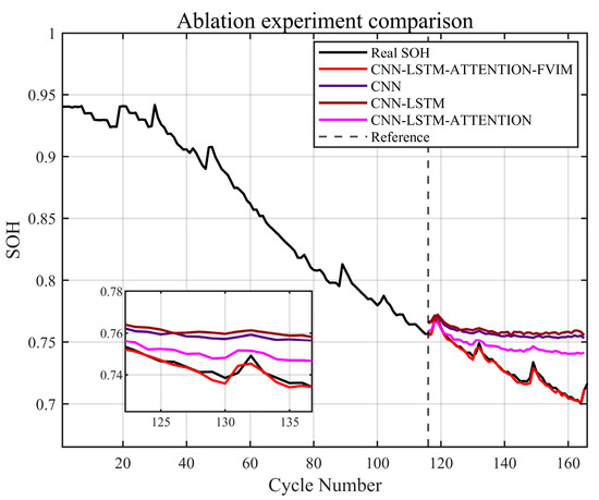
Figure 12.
Ablation experiment comparison chart.
Table 7.
Ablation experiment evaluation indicators.
At the same time, we recorded the total running time of each model in the ablation experiment in Table 8. Although the total running time of the model proposed in this article is slightly higher than that of the other models, this increase is reasonable because the accuracy has been significantly improved, and the extra time is within an acceptable range. It is worthwhile to accept a slightly higher time cost for a higher prediction accuracy.
Table 8.
Total running time.
6. Conclusions
In order to solve the problem of insufficient prediction accuracy of lithium-ion battery state of health (SOH), this study proposed an innovative method for estimating lithium-ion battery SOH based on the CNN-LSTM-Attention-FVIM algorithm and multiple feature fusion. The following are the main conclusions:
- By analyzing the battery charging curve and related health factors, and using the Pearson and Spearman correlations to analyze the correlation with its SOH, the health factors with lower correlation were eliminated, and the input data quality was optimized.
- In order to solve the problems of prediction fluctuation and large error caused by the randomness of the parameters of the traditional CNN-LSTM-Attention model and the inability to find the optimal parameters, the FVIM algorithm was introduced to globally optimize its input weights and biases, and key parameters such as learning rate, regularization coefficient, and number of hidden layer nodes were dynamically adjusted to achieve the best prediction effect.
- By comparing the advantages and disadvantages of the proposed model with four deep learning network models, namely GRU, BILSTM, CNN, and CNN-LSTM-Attention, the proposed method had the smallest SOH estimation error.
- When the proposed model as used to predict and estimate battery SOH for different batteries and different training set ratios, its RMSE and MAE were less than 0.99% and 1.33%, respectively.
This method has been verified using the NASA and University of Maryland battery aging datasets, showing strong fitting characteristics, multi-condition compatibility, and excellent prediction capabilities. However, faced with the challenge of random fragmented charging data (such as 20–80% partial charging) in practical applications, in the future, we will focus on developing lightweight optimization strategies such as feature reconstruction technology based on generative adversarial networks to improve real-time performance and generalization across battery models, promoting the sustainable development of electric vehicles and energy storage systems.
Author Contributions
G.L.: conceptualization, experiment, validation, writing—original draft. Z.D.: resources, methodology, writing—review and editing, supervision. L.L.: methodology, validation, resources. Y.X.: validation, supervision, writing—review and editing. G.G.: methodology, validation, supervision. H.Z.: experiment, software, writing—review and editing. L.T.: resources, conceptualization. Y.L.: experiment, software. M.G.: Writing—review and editing. Z.Y.: Experiment, methodology. M.Y.: validation, supervision. All authors have read and agreed to the published version of the manuscript.
Funding
This work was sponsored by the Beijing Natural Science Foundation (Grant 3244039), “R&D Program of Beijing Municipal Education Commission” (Grant KM202411232021), Collaborative Innovation Center of Ningde Normal University (Grant 2022ZX02).
Institutional Review Board Statement
Not applicable.
Informed Consent Statement
Not applicable.
Data Availability Statement
The data provided in this study are available on NASA’s official website and the University of Maryland’s official website. These data are derived from the following available resources in the public domain: https://ti.arc.nasa.gov/tech/dash/groups/pcoe/prognostic-data-repository/#battery and https://calce.umd.edu/battery-data.
Conflicts of Interest
The authors declare that they have no known competing financial interests or personal relationships that could have appeared to influence the work reported in this paper.
References
- Xu, Y.H.; Fang, J.; Zhang, H.G.; Song, S.S.; Tong, L.; Peng, B.Y.; Yang, F.B. Experimental investigation on the output performance of a micro compressed air energy storage system based on a scroll expander. Renew. Energy 2025, 243, 122602. [Google Scholar] [CrossRef]
- Zhang, Y.; Li, Y.F. Prognostics and health management of Lithium-ion battery using deep learning methods: A review. Renew. Sustain. Energy Rev. 2022, 161, 112282. [Google Scholar] [CrossRef]
- Sun, X.W.; Zhang, Y.; Zhang, Y.C.; Wang, L.C.; Wang, K. Summary of health-state estimation of lithium-ion batteries based on electrochemical impedance spectroscopy. Energies 2023, 16, 5682. [Google Scholar] [CrossRef]
- Qu, J.T.; Liu, F.; Ma, Y.X.; Fan, J.M. A neural-network-based method for RUL prediction and SOH monitoring of lithium-ion battery. IEEE Access 2019, 7, 87178–87191. [Google Scholar] [CrossRef]
- Peng, S.M.; Chen, S.D.; Liu, Y.; Yu, Q.Q.; Kan, J.; Li, R. State of power prediction joint fisher optimal segmentation and PO-BP neural network for a parallel battery pack considering cell inconsistency. Appl. Energy 2025, 381, 125130. [Google Scholar] [CrossRef]
- Zuo, H.Y.; Liang, J.; Zhang, B.; Wei, K.X.; Zhu, H.; Tan, J.Q. Intelligent estimation on state of health of lithium-ion power batteries based on failure feature extraction. Energy 2023, 282, 128794. [Google Scholar] [CrossRef]
- Tian, J.P.; Xiong, R.; Shen, W.X. State-of-health estimation based on differential temperature for lithium ion batteries. IEEE Trans. Power Electron. 2020, 35, 10363–10373. [Google Scholar] [CrossRef]
- Zou, Y.; Hu, X.S.; Ma, H.M.; Eben Li, S.E. Combined state of charge and state of health estimation over lithium-ion battery cell cycle lifespan for electric vehicles. J. Power Sources 2015, 273, 793–803. [Google Scholar] [CrossRef]
- Li, Q.L.; Li, D.Z.; Zhao, K.; Wang, L.C.; Wang, K. State of health estimation of lithium-ion battery based on improved ant lion optimization and support vector regression. J. Energy Storage 2022, 50, 104215. [Google Scholar] [CrossRef]
- Peng, S.M.; Zhang, D.H.; Dai, G.H.; Wang, L.; Jiang, Y.X.; Zhou, F. State of charge estimation for LiFePO4 batteries joint by PID observer and improved EKF in various OCV ranges. Appl. Energy 2025, 377, 124435. [Google Scholar] [CrossRef]
- Wu, J.; Cui, X.C.; Meng, J.H.; Peng, J.C.; Lin, M.Q. Data-driven transfer-stacking-based state of health estimation for lithium-ion batteries. IEEE Trans. Ind. Electron. 2023, 71, 604–614. [Google Scholar] [CrossRef]
- Yang, D.; Zhang, X.; Pan, R.; Wang, Y.J.; Chen, Z.H. A novel Gaussian process regression model for state-of-health estimation of lithium-ion battery using charging curve. J. Power Sources 2018, 384, 387–395. [Google Scholar] [CrossRef]
- Gou, B.; Xu, Y.; Feng, X. State-of-health estimation and remaining-useful-life prediction for lithium-ion battery using a hybrid data-driven method. IEEE Trans. Veh. Technol. 2020, 69, 10854–10867. [Google Scholar] [CrossRef]
- Fan, Y.X.; Xiao, F.; Li, C.R.; Yang, G.R.; Tang, X. A novel deep learning framework for state of health estimation of lithium-ion battery. J. Energy Storage 2020, 32, 101741. [Google Scholar] [CrossRef]
- Zhang, S.X.; Liu, Z.T.; Xu, Y.; Chen, G.W.; Su, H.Y. An Electrochemical Aging-Informed Data-Driven Approach for Health Estimation of Lithium-Ion Batteries with Parameter Inconsistency. IEEE Trans. Power Electron. 2025, 40, 7354–7369. [Google Scholar] [CrossRef]
- Liu, Y.M.; Chen, H.L.; Yao, L.G.; Ding, J.X.; Chen, S.Q.; Wang, Z.Y. A physics-guided approach for accurate battery SOH estimation using RCMHCRE and BatteryPINN. Adv. Eng. Inform. 2025, 65, 103211. [Google Scholar] [CrossRef]
- Tran, M.K.; Mathew, M.; Janhunen, S.; Panchal, S.; Raahemifar, K.; Fraser, R.; Fowler, M. A comprehensive equivalent circuit model for lithium-ion batteries, incorporating the effects of state of health, state of charge, and temperature on model parameters. J. Energy Storage 2021, 43, 103252. [Google Scholar] [CrossRef]
- Li, C.F.; Yang, L.; Li, Q.; Zhang, Q.S.; Zhou, Z.Y.; Meng, Y.Z.; Zhao, X.W.; Wang, L.; Zhang, S.M.; Li, Y.; et al. SOH estimation method for lithium-ion batteries based on an improved equivalent circuit model via electrochemical impedance spectroscopy. J. Energy Storage 2024, 86, 111167. [Google Scholar] [CrossRef]
- Chen, M.Z.; Ma, G.J.; Liu, W.B.; Zeng, N.Y.; Luo, X. An overview of data-driven battery health estimation technology for battery management system. Neurocomputing 2023, 532, 152–169. [Google Scholar] [CrossRef]
- Li, D.Z.; Yang, D.F.; Li, L.W.; Wang, L.C.; Wang, K. Electrochemical impedance spectroscopy based on the state of health estimation for lithium-ion batteries. Energies 2022, 15, 6665. [Google Scholar] [CrossRef]
- Tan, Y.D.; Zhao, G.C. Transfer learning with long short-term memory network for state-of-health prediction of lithium-ion batteries. IEEE Trans. Ind. Electron. 2019, 67, 8723–8731. [Google Scholar] [CrossRef]
- Guo, Y.; Yang, D.F.; Zhang, Y.; Wang, L.C.; Wang, K. Online estimation of SOH for lithium-ion battery based on SSA-Elman neural network. Prot. Control Mod. Power Syst. 2022, 7, 40. [Google Scholar] [CrossRef]
- Li, P.H.; Zhang, Z.J.; Xiong, Q.Y.; Ding, B.C.; Hou, J.; Luo, D.C.; Rong, Y.J.; Li, S.Y. State-of-health estimation and remaining useful life prediction for the lithium-ion battery based on a variant long short term memory neural network. J. Power Sources 2020, 459, 228069. [Google Scholar] [CrossRef]
- Shen, P.; Ouyang, M.G.; Lu, L.G.; Li, J.Q.; Feng, X.N. The co-estimation of state of charge, state of health, and state of function for lithium-ion batteries in electric vehicles. IEEE Trans. Veh. Technol. 2017, 67, 92–103. [Google Scholar] [CrossRef]
- Li, X.Y.; Wang, Z.P.; Zhang, L.; Zou, C.F.; Dorrell, D.D. State-of-health estimation for Li-ion batteries by combing the incremental capacity analysis method with grey relational analysis. J. Power Sources 2019, 410, 106–114. [Google Scholar] [CrossRef]
- Su, S.S.; Li, W.; Mou, J.H.; Garg, A.; Gao, L.; Liu, J. A hybrid battery equivalent circuit model, deep learning, and transfer learning for battery state monitoring. IEEE Trans. Transp. Electrif. 2022, 9, 1113–1127. [Google Scholar] [CrossRef]
- Sui, X.; He, S.; Vilsen, S.B.; Meng, J.H.; Teodorescu, R.; Stroe, D.I. A review of non-probabilistic machine learning-based state of health estimation techniques for Lithium-ion battery. Appl. Energy 2021, 300, 117346. [Google Scholar] [CrossRef]
- Xu, H.W.; Wu, L.F.; Xiong, S.Z.; Li, W.; Garg, A.; Gao, L. An improved CNN-LSTM model-based state-of-health estimation approach for lithium-ion batteries. Energy 2023, 276, 127585. [Google Scholar] [CrossRef]
- Sun, C.Y.; Lu, T.L.; Li, Q.B.; Liu, Y.L.; Yang, W.; Xie, J.Y. Predicting the Future Capacity and Remaining Useful Life of Lithium-Ion Batteries Based on Deep Transfer Learning. Batteries 2024, 10, 303. [Google Scholar] [CrossRef]
- Stroebl, F.; Petersohn, R.; Schricker, B.; Schaeufl, F.; Bohlen, O.; Palm, H. A multi-stage lithium-ion battery aging dataset using various experimental design methodologies. Sci. Data 2024, 11, 1020. [Google Scholar] [CrossRef]
- Ren, Z.; Du, C.Q. A review of machine learning state-of-charge and state-of-health estimation algorithms for lithium-ion batteries. Energy Rep. 2023, 9, 2993–3021. [Google Scholar] [CrossRef]
- Wang, S.L.; Ren, P.; Takyi-Aninakwa, P.; Jin, S.Y.; Fernandez, C. A critical review of improved deep convolutional neural network for multi-timescale state prediction of lithium-ion batteries. Energies 2022, 15, 5053. [Google Scholar] [CrossRef]
- Tang, X.P.; Liu, K.L.; Lu, J.Y.; Liu, B.Y.; Wang, X.; Gao, F.R. Battery incremental capacity curve extraction by a two-dimensional Luenberger–Gaussian-moving-average filter. Appl. Energy 2020, 280, 115895. [Google Scholar] [CrossRef]
- Ma, L.L.; Xu, Y.H.; Zhang, H.G.; Yang, F.B.; Wang, X.; Li, C. Co-estimation of state of charge and state of health for lithium-ion batteries based on fractional-order model with multi-innovations unscented Kalman filter method. J. Energy Storage 2022, 52, 104904. [Google Scholar] [CrossRef]
- Song, X.B.; Yang, F.F.; Wang, D.; Tsui, K.L. Combined CNN-LSTM network for state-of-charge estimation of lithium-ion batteries. IEEE Access 2019, 7, 88894–88902. [Google Scholar] [CrossRef]
- Chemali, E.; Kollmeyer, P.J.; Preindl, M.; Ahmed, R.; Emadi, A. Long short-term memory networks for accurate state-of-charge estimation of Li-ion batteries. IEEE Trans. Ind. Electron. 2017, 65, 6730–6739. [Google Scholar] [CrossRef]
- Li, F.; Zuo, W.; Zhou, K.; Li, Q.Q.; Huang, Y.H. State of charge estimation of lithium-ion batteries based on PSO-TCN-Attention neural network. J. Energy Storage 2024, 84, 110806. [Google Scholar] [CrossRef]
- Fakhouri, H.N.; Awaysheh, F.M.; Alawadi, S.; Alkhalaileh, M.; Hamad, F. Four vector intelligent metaheuristic for data optimization. Computing 2024, 106, 2321–2359. [Google Scholar] [CrossRef]
Disclaimer/Publisher’s Note: The statements, opinions and data contained in all publications are solely those of the individual author(s) and contributor(s) and not of MDPI and/or the editor(s). MDPI and/or the editor(s) disclaim responsibility for any injury to people or property resulting from any ideas, methods, instructions or products referred to in the content. |
© 2025 by the authors. Licensee MDPI, Basel, Switzerland. This article is an open access article distributed under the terms and conditions of the Creative Commons Attribution (CC BY) license (https://creativecommons.org/licenses/by/4.0/).