Assessment of Bone Aging—A Comparison of Different Methods for Evaluating Bone Tissue

Abstract

This study tackles the challenge of automatically estimating age from pelvis radiographs. Furthermore, we aim to develop a methodology for applying artificial intelligence to classify or regress medical imagery data. Our dataset comprises 684 pelvis X-ray images of patients, each accompanied by annotations and masks for various regions of interest (e.g., the femur shaft). Radiomic features, e.g., the co-occurrence matrix, were computed to characterize the image content. We assessed statistical analysis, machine learning, and deep learning methods for their effectiveness in this task. Correlation analysis indicated that using certain features in specific regions of interest is promising for accurate age estimation. Machine learning models demonstrated that when using uncorrelated features, the optimal mean absolute error (MAE) for age estimation is 5.20, whereas when employing convolutional networks on the texture feature maps yields the best result of 9.56. Automatically selecting radiomic features for machine learning models achieves a MAE of 7.99, whereas utilizing well-known convolutional architectures on the original image results in a system efficacy of 7.96. The use of artificial intelligence in medical data analysis produces comparable outcomes; however, when dealing with a large number of descriptors, selecting the most optimal ones through statistical analysis enables the identification of the best solution quickly.

1. Introduction

Bone age assessment has long served as a cornerstone of clinical evaluation in pediatric endocrinology, orthopedics, and forensic medicine. Traditional approaches rely heavily on standardized methods such as the Greulich–Pyle (GP) atlas and the Tanner-Whitehouse (TW) scoring systems, both of which focus on hand and wrist radiographs of growing children. While these methods remain widely used, they are often limited by subjectivity, inter-rater variability, and inapplicability beyond puberty [1,2]. As such, their relevance diminishes considerably in adult populations, where skeletal maturity precludes the use of classic growth markers.

Attempts to assess age based on the analysis of X-ray images have already been undertaken, mainly in the context of forensic medicine. Li-Qin estimated the chronological age based on annealing of pelvic X-rays. However, the study was designed to show that image segmentation improves estimation accuracy and was limited to cases aged 11–21 years [3]. Other studies have mainly focused on the use of deep learning and artificial intelligence methods in age assessments based on X-ray images [4,5].

Recent advances in artificial intelligence (AI) and image processing have reinvigorated the field, offering new methods for bone age estimation across a broader demographic spectrum. Most of these developments, however, continue to concentrate on hand X-rays and pediatric datasets. For instance, Dehghani et al. [6] proposed a fully automated system for age assessment from infancy through adolescence, and Hui et al. [7] introduced a global–local convolutional neural network tailored for hand radiographs, showing excellent accuracy in growing individuals. Mao et al. [8] further expanded this frontier using a transformer-based architecture to refine attention on skeletal landmarks. Despite these technical improvements, they offer limited applicability for adult or elderly subjects, especially when radiographic landmarks associated with skeletal growth have fused.

In parallel, meta-analyses such as those by Prokop-Piotrkowska et al. [9] have underscored the urgent need for validated methodologies that extend beyond pediatric applications, particularly in forensic and medico-legal settings, where adult age estimation is increasingly required. Franklin et al. [10] emphasize that in living individuals, especially adults, there is no universally accepted or standardized radiographic method for chronological age estimation—highlighting the demand for new anatomical targets and analytical strategies.

In response to these limitations, our work proposes a novel approach: utilizing pelvic radiographs (both CR—computed radiography—and DR—digital radiography—modalities) for age estimation based on trabecular bone texture features. The pelvic skeleton offers a promising alternative, as it retains microarchitectural changes related to bone remodeling, mineral density, and degenerative processes across the lifespan. This approach is grounded in our previous findings, which identified significant correlations between patient age and textural features extracted from the femoral head and acetabular regions [11,12]. Most notably, autoregressive texture descriptors—particularly ARM Theta 1—showed robust and repeatable correlations with age (up to r = 0.72 in selected subgroups), highlighting the sensitivity of pelvic trabecular architecture to chronological aging.

The biological and skeletal ages of bones usually correlate with chronological age. This fact can be used in forensic medicine studies [13]. However, certain diseases, such as parathyroid dysfunction or kidney disease, can significantly impact bone health [14,15]. This, in turn, means that chronological age may not correspond to the biological state of the bone. This knowledge can be invaluable, for example, in planning alloplasty and selecting the appropriate type of implant [16]. Importantly, this pelvic-based method also holds promise for broader clinical and forensic applications. It is anatomically stable, less susceptible to deformities common in peripheral bones, and routinely available in preoperative imaging, especially in orthopedic patients. Furthermore, the use of high-resolution DR systems enhances the reliability of texture analysis and facilitates large-scale, retrospective studies without additional radiation exposure.

By integrating radiomic analysis with population-based anatomical insight, our study bridges a crucial gap in bone age estimation: the need for reliable, reproducible, and interpretable tools applicable to skeletally mature individuals. In doing so, it complements the existing body of AI-driven research and offers a novel, anatomically grounded perspective on adult age estimation. In the study, we assumed that chronological age corresponds to biological bone age. A situation in which the age assessed based on X-ray exceeds the chronological age suggests that the bone quality (understood as biological age) does not correspond to that expected based on chronological age. This paper highlights two main accomplishments. First, we show that accurately estimating a patient’s age from pelvic X-rays is feasible. Secondly, we introduce a methodology for selecting appropriate regions of interest (ROIs) when examining medical data. We are confident that this methodology could be applied to all visual modalities in medicine, with radiograms serving as a practical demonstration of its utility.

2. Materials and Methods

This section provides a concise summary of the research methods employed. We begin with a description of the methodology, followed by a detailed explanation of each component: statistical analysis, texture feature extraction, the machine learning approach, and finally, the deep learning approach. Also, we would like to offer comprehensive information about the dataset used in this study.

2.1. Research Methodology

Figure 1 illustrates the key steps of the proposed methodology. Initially, choosing some easily accessible ROIs or those that appear relevant based on the problem description was recommended. Conducting a correlation analysis between textural features derived from these ROIs and the target values helps determine if one was on the right track to achieving the goal. This phase of the research was also relatively quick. Once it was established that further exploration is worthwhile, the results of traditional machine learning, which relies on textural features, were compared with those from a deep learning approach to analyze image patches. In our research, both methods support the initial assumptions drawn from the correlation analysis; however, depending on the dataset and sample size, one approach may yield superior results. Ultimately, when it is appropriate to apply artificial intelligence, the positioning of ROIs for automated data analysis could be refined.

2.2. Dataset

During routine examinations at the Małopolska Orthopaedic and Rehabilitation Hospital from July 2022 to February 2023, pelvic DR images were collected. This made it possible to avoid exposing the patient to an additional dose of X-ray; moreover, it allowed for collecting the chronological age, which served as the reference point for the results. These images were captured using the Visaris Avanse DR (Visaris, Serbia) and stored in DICOM (Digital Imaging and Communication in Medicine) format as 12-bit (16-bit allocated) data with a pixel spacing of 0.13256 × 0.13256 mm². For further analysis, the images were scaled down to 8 bits by using the minimum and maximum values to establish the range. 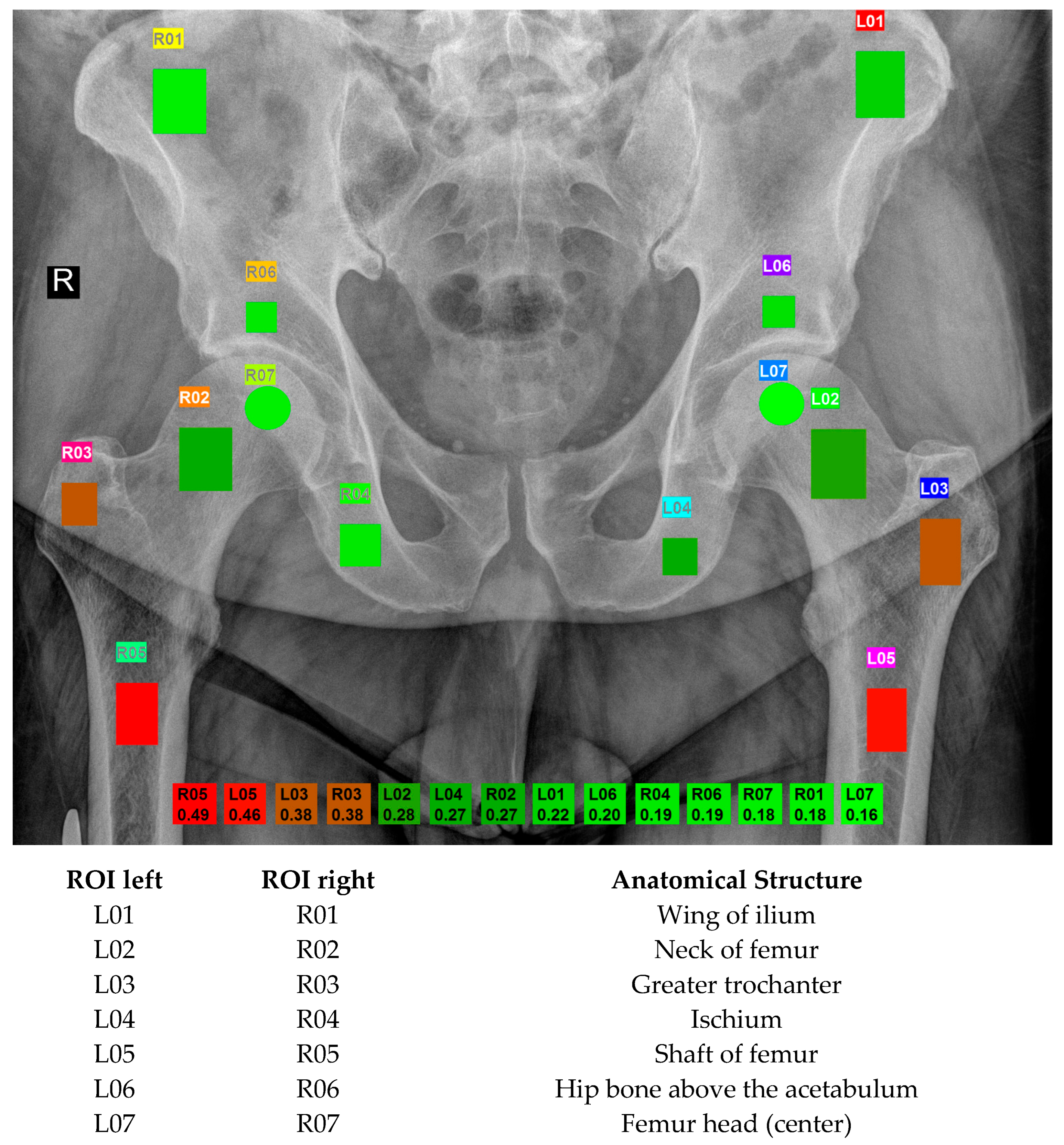Additionally, the original images underwent further enhancement, as detailed in [12]. Each image includes twelve rectangular and two circular ROIs, carefully annotated with the assistance of MaZda 19.02 software [17] (see Figure 2 for details). Radiologists with a minimum of six years of experience in musculoskeletal structures chose those regions. The placement and the size of the ROI depended on the anatomical structure. The clinical importance and changes that occur in the bone with age dictated the choice of ROIs. Osteoporosis primarily leads to the loss of spongy bone resulting in weakened bones. ROI 01 (wing of ilium) and 04 (ischium) are areas used to assess bone quality in general and serve as reference points. ROI 02 corresponds to the femoral neck, which is standardly assessed in a densitometry examination, while ROI 03 is mainly composed of spongy bone in the greater trochanter. In turn, ROI 05 is the region of the femur where the stem of a classic hip joint endoprosthesis is stabilized. ROI 06 (hip bone above the acetabulum) is mostly cancellous bone, in which the acetabulum of the endoprosthesis is embedded and stabilized. ROI 07 represents the femoral head, susceptible to possible degenerative and necrotic changes.

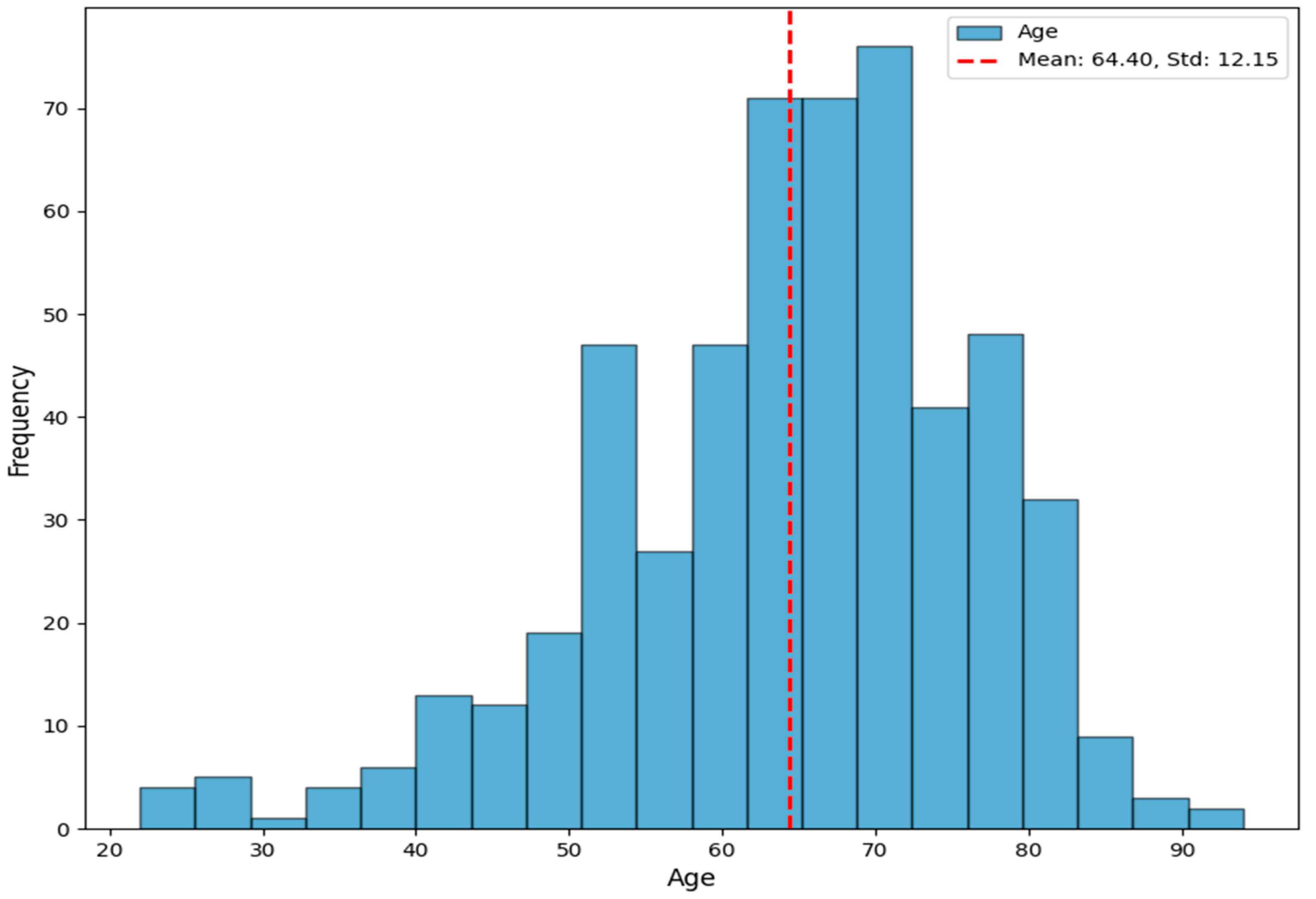
Although the dataset contains 684 images, only 480 are free of artifacts in the research area, which excludes the others from consideration. The ages of the patients range from 22 to 94, with an average age of 64.40 ± 12.15. There are 273 females and 207 males in this cohort. Figure 3 presents the age distribution in the dataset. All individuals are Caucasian. A medical annotation includes the patient’s age. The dataset is accessible at Zendo DOI: https://doi.org/10.5281/zenodo.15352880.

2.3. Texture Features

The pyRadiomics [18] library simplifies the calculation of textural features. Since these features are widely recognized, we direct interested readers to other sources [18,19,20] where the details concerning first-order features, the grey-level co-occurrence matrix, the gray-level size zone matrix, the gray level run length matrix, the gray-level dependence matrix, the neighboring gray-tone difference matrix, gradient map features, the first-model auto-regressive model, the Haar wavelet transform, the Gabor transform, and the histogram of oriented gradients are described.

When dealing with small image patches, indicated by the mask, and when data came from different systems, it was crucial to standardize illumination variations. In our study, we employed normalization techniques (HEQ—histogram equalization, CLAHE—contrast-limited adaptive histogram equalization, and SDA—statistical dominance algorithm [21]) as well as ROI normalization using mean value and standard deviation, min-max image normalization, and excluding the first and last percentiles from the histogram, as described in Section 2.4. Additionally, the reduction in bit depth affects the descriptive quality of textural features [22,23]. Therefore, we calculated the features separately for data quantized from five to eight bits.

2.4. Image Normalization

Similarly to the previous study [12], we investigated the influence of various image normalization techniques. These techniques aimed to improve image contrast, which in turn leads to better visualization of bone trabeculation. We performed the tests using algorithms such as adaptive HEQ, its contrast-limited version CLAHE, and the statistical dominance algorithm (SDA). The SDA enhances image edges and reduces the impact of uneven background brightness distribution [8]. The entire image followed these transformations.

Normalization of the region of interest (ROI) was also implemented. It is essential and often used in the case of texture analysis. In this way, it is possible to limit the influence of differences in brightness and contrast that may occur in the ROI images acquired for different patients. As a result, normalization limits the dependence of the computed texture parameters on the ROI brightness and contrast, ensuring that these parameters more accurately describe the structure of the visualized tissue [18]. The normalization leads to the extension of the ROI gray levels to the entire available range of image brightness, according to the following equation:

$$N\left(x,y\right)=round{\displaystyle \frac{I\left(x,y\right)-{min}_{norm}}{{max}_{norm}-{min}_{norm}}},$$

(1)

where N(x,y) and I(x,y) are normalized and original images, respectively, and min_norm and max_norm represent minimum and maximum normalized gray-level value.

This study used three types of ROI normalization, leading to different determinations of min_norm and max_norm:

• Min–max: in this type of normalization, the min_norm and max_norm are the minimum and maximum intensities taken directly from the histogram.
• Percentile: in this case the min_norm and max_norm values are determined based on the cumulative histogram corresponding to the 1% and 99% percentiles, respectively.
• Mean: the range of intensities for this normalization can be defined as min_norm = µ − 3σ and max_norm = µ + 3σ, where µ is the mean intensity and σ is the standard deviation of the image intensities in the ROI.

Since limiting the number of bits/pixels in some cases reduces noise in textured images, we also performed these analyses for different ranges of ROI brightness.

2.5. Statistical Analysis

We performed a statistical analysis to evaluate the relationship between patient age and textural features extracted from ROIs. Approximately 300 features were computed for each manually annotated ROI.

Before conducting the correlation assessment, the Shapiro–Wilk test was used to check the distribution of each feature. Based on normality, the following correlation coefficients were applied: Pearson’s correlation for normally distributed features and Spearman’s or Kendall’s correlation for non-parametric data. When the feature contained repeated values, Kendall’s coefficient was used. The strength of the correlation was interpreted as moderate (0.3–0.5) or strong (>0.5). A two-tailed test was used to evaluate the statistical significance of correlations, with a p-value threshold of 0.05 considered statistically significant.

Given the paired data (x, y), the Pearson and the Kendall correlation coefficients are defined by the following formulae:

$$Pearson={\displaystyle \frac{\sum (x_i-\overline{x})(y_i-\overline{y})}{\sqrt{\sum {(x_i-\overline{x})}^2{(y_i-\overline{y})}^2}}},$$

(2)

$$Kendall={\displaystyle \frac{\left(No.ofconcordantpairs\right)-(No.ofdiscorantpairs)}{(No.ofpairs)}},$$

(3)

while the Spearman correlation is defined as a Pearson correlation for variables that are ranked.

All statistical computations were performed using R (R Core Team, 2024, version 4.4.1), and RStudio (RStudio Team, 2023, version 2023.6.1.524).

2.6. Machine Learning

Estimating age is a regression challenge, where values within a specific range are identified from a feature vector. To ensure a comprehensive analysis, we considered several techniques, including Logistic Regression, Random Forests, Support Vector Machines (utilizing both linear and radial basis function kernels), Multiple Perceptron, Gradient Boost, AdaBoost, and XGBoost. Utilizing a wide range of methods allowed us to conduct an accurate assessment of the issue. Given that textural features characterized the feature vectors derived from image patches, they tend to be quite lengthy, especially when compared to the number of samples in the dataset. A large number of features posed a challenge for standard machine learning regression methods. Consequently, we opted to experiment with various feature extraction techniques to identify 10 features to input into the regression method. In our research, we employed both univariate (Fisher, Spearman, Pearson, Kendall) and multivariate feature selection methods (mutual information maximization—MIM, max-relevance and min-redundancy—MRMR, mutual joint information—MJI, conditional information feature extraction—CIFE), as well as principal component analysis—PCA.

2.7. Deep Learning

We cut the area of the mask from the original image to prepare the training data. A few of the images were missing specific masks; thus, they were discarded. We transformed circular ROIs to squares by cutting the rectangular area based on the circumference of the circle. We ensured that all masks were filled with data that originated from the image. No black background was accepted.

Since each patient’s anatomy is unique, no single mask can be of the same size. To train the model in batches, a single size was assumed for a given type of mask. Smaller and bigger masks were slightly resized to this value. Based on average mask size, values of 96 × 96 were chosen.

Selected model architectures were adapted from the Torchvision library, but the fully connected layers were modified to solve the regression problem. One hidden layer was added, which improved feature extraction and results. In deep learning, when utilizing a specific model architecture, one has the option to use either randomly initialized weights or weights derived from previous model training for a different task. The transfer learning approach provides a model that, while not initially well-prepared to solve a new problem, has prior experience with similar tasks, thereby facilitating its adaptation to new challenges. Typically, in this setting, the first dataset is large, whereas the second may be significantly smaller. The ImageNet dataset is widely used to evaluate network capabilities in classification tasks, allowing for the acquisition of various network models with weights already pre-trained on these data. Various models were tested, like ResNet34 [24], ResNet50 [24], ConvNext_Tiny [25], ResNext50_32x4d [26], EfficientNet_b0 [27], EfficientNet_v2_s [28].

To ensure reproducibility and fairness of results across all experiments, a consistent random seed was used across all runs. The optimizer used was AdamW with a weight decay parameter of 0.01 to prevent overfitting. The initial learning rate was set to 0.0001, and the model was trained for 35 epochs. A quite small number of epochs was chosen due to the limited amount of data. The ReduceLROnPlateau learning rate scheduler was used to adaptively reduce the learning rate when the validation loss did not improve over time. The patience parameter for this scheduler was set to 3. The best-performing criterion was mean squared error (MSELoss). The effectiveness is likely attributed to the high quality of the dataset, with labels carefully prepared to minimize errors. The early stopping technique was not used during training. Model selection for testing was chosen based on the lowest validation loss during training.

2.8. Experiment Methodology

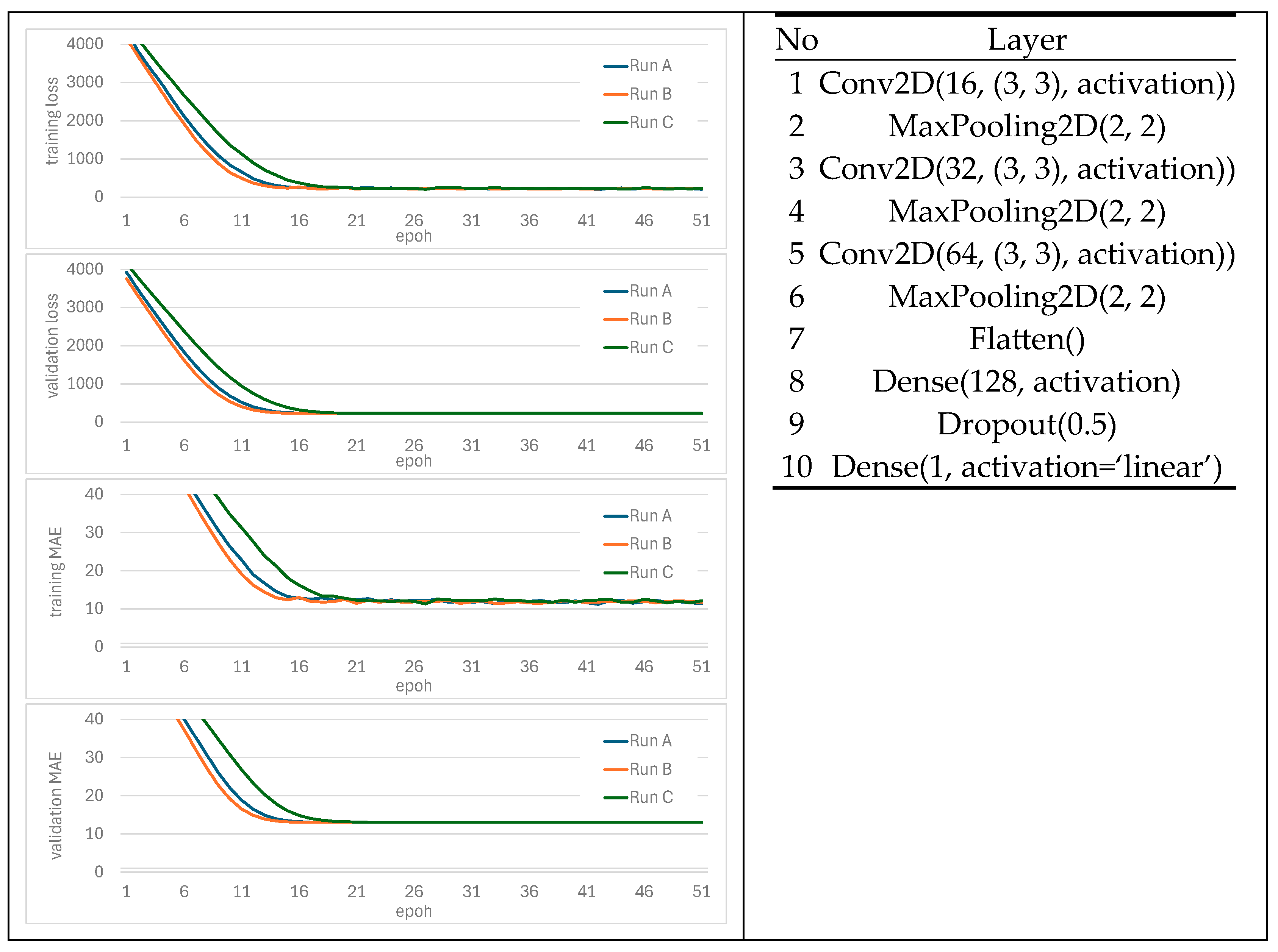
All experiments performed in this study follow a five-fold cross-validation approach. When the standard machine learning approach was used, one fold was designated as the testing set, while the remaining four were used for training. In the case of deep learning, validation samples originated from a training dataset split at a ratio of 0.2. This setting allows for easy comparison between results obtained in all considered settings. When working with statistical features (see Section 3.2), each fold was trained three times for 200 epochs without early stopping. The optimizer was Adam with default no weight decay, and the learning rate was set to 0.00001. The batch size was equal to 32. The loss function was the mean square error (MSE), and the metric was the mean absolute error (MAE).

The quality of each model is presented as the average of results obtained from each fold, using the following metrics: mean absolute error (MAE), mean absolute percentage error (MAPE,) and the coefficient of determination (R2). Using a dataset of N samples, the metric compares the actual T value with a prediction P returned by the model in the following manner:

$$MAE={\displaystyle \frac{1}{N}}\sum \left|P-T\right|,$$

(4)

$$MAPE={\displaystyle \frac{1}{N}}\sum \left|{\displaystyle \frac{T-P}{T}}\right|,$$

(5)

$$R2=1-{\displaystyle \frac{\sum {\left(T_i-P_i\right)}^2}{\sum \left(T_i-\overline{T}\right)}},$$

(6)

where $\overline{T}$ is the average of known values.

3. Results

This section provides an overview of the experiments conducted to determine the most effective method for estimating age from pelvic radiographs. Initially, we examined whether there were any correlations between age and certain radiomic features that could characterize the data. With the identification of the most effective ROIs and promising textural features, we explored simple machine learning and deep learning techniques to assess the feasibility of age estimation. Subsequently, we employed a global machine learning approach to determine if automatically selecting uncorrelated features and training models aligned with our findings. Finally, we evaluated several well-established deep learning architectures to assess their suitability. We conclude this section with a discussion on the automatic identification of optimal ROIs.

3.1. Statistical Analysis

The correlation analysis performed on approximately 300 textural features calculated for each manually annotated ROI revealed several significant relationships with patient age. The Pearson, Spearman, and Kendall correlation coefficients were computed depending on the feature distribution, as described in Section 2.5.

The results are summarized in

Table 1. The statistical evaluation of correlation between the features in the ROI and patient age.

ROI	Anatomical Structure	$\mathbf{Pearson}\mathbf{Coefficient}\uparrow$	$\mathbf{Spearman}\mathbf{Coefficient}\uparrow$	$\mathbf{Kendall}\mathbf{Coefficient}\uparrow$
L01	Left wing of ilium	0.22	0.25	0.17
L02	Left neck of femur	0.28	0.26	0.18
L03	Left greater trochanter	0.38	0.35	0.24
L04	Left ischium	0.27	0.26	0.18
L05	Left shaft of femur	0.46	0.40	0.32
L06	Left hip bone above the acetabulum	0.20	0.19	0.12
L07	Left femur head (center)	0.16	0.20	0.13
R01	Right wing of ilium	0.18	0.19	0.14
R02	Right neck of femur	0.27	0.24	0.18
R03	Right greater trochanter	0.38	0.37	0.25
R04	Right ischium	0.20	0.24	0.17
R05	Right shaft of femur	0.49	0.47	0.34
R06	Right hip bone above the acetabulum	0.19	0.20	0.15
R07	Right femur head (center)	0.18	0.26	0.14

. The strongest correlations were observed using Pearson’s coefficient. The best-performing ROIs were the right femoral shaft (R05) and the left femoral shaft (L05), with correlation coefficients of 0.49 and 0.46, respectively. Next, a meaningful relationship was found for the greater trochanter (R03 and L03). The analysis confirmed that a moderate correlation strength (r = 0.3–0.5) was observed for several ROIs, with R05 achieving the highest correlation. All correlation coefficients presented in Table 1 are statistically significant with p ≤ 0.001. Figure 2 illustrates the Pearson correlation coefficients across all evaluated ROIs visually.

One of our goals was to check the impact of preprocessing methods, similar to what we did in our previous work [12]. Therefore, we conducted several experiments both without preprocessing and with operations such as HEQ, CLAHE, their combination (CLAHE and HEQ), and SDA. The results indicated that preprocessing did not provide a significant improvement. Specifically, there was no significant improvement in correlation for the most critical ROI, ROI 05 (R05: none–0.49, CLAHE/HEQ—0.49, SDA—0.497; L05: none–0.46, CLAHE/HEQ—0.46, SDA—0.46). However, this correlation improved for the second ROI, ROI 03 (R03: none–0.38, CLAHE/HEQ—0.43, SDA—0.44; L03: none–0.38, CLAHE/HEQ—0.39, SDA—0.41). For the remaining ROIs, a positive change was noted, but in these cases, the correlation value did not exceed 0.3. Therefore, we limited the presentation to the results obtained without preprocessing. Additionally, we assessed whether patient sex influenced the correlation between textural features and age. The most age-dependent ROIs (R05 and R03, L05 and L03) were not related to sex. However, a slight impact of sex was noted. In the male group, there was a noticeably higher correlation with age for L01, L02, and R01, as well as a higher correlation for R02 (although lower than for R/L05 and R/L03, it was not high enough to be considered significant). These results were not observed in the female group. This is consistent with previous findings [12].

Among the texture features, the most frequently best correlating textural features were the Teta 1 and Sigma AutoRegressive Model (ARM) features, as well as the Local Binary Pattern (LBP) group features.

3.2. Age Estimation on the Statistically Suggested Features

We selected ten textural features with the highest correlation values for the optimal ROIs identified through statistical analysis (L/R03 and L/R05).

Table 2. The best uncorrelated textural features for the selected ROIs (03—greater trochanter, 05—shaft of femur).

L03	L05	R03	R05
Yc5LbpCs8n5	Ys10M7ArmTeta2	Yc5LbpCs8n13	Yc5LbpCs8n5
Yc5LbpCs8n11	Ys10M8ArmTeta1	Yc5LbpCs8n11	Yc5LbpCs8n13
Yc5LbpCs8n4		Yc5LbpCs8n9	Yc5LbpCs8n9
Yc5LbpOc4n9		Yc5M7GlcmV2InvDfMom	Yc5LbpOc4n15
		Yc5M7GlcmN1InvDfMom
		Yc5M6GrlmVShrtREmp

presents the uncorrelated representations for each ROI. Given that the resolution of the ROIs varies by patient, a maximum common resolution was established (L03: 75 × 121, L05: 64 × 108, R03: 71 × 123, R05: 62 × 107). All masks were then adjusted to a uniform size, assuming that the centers of the original and smaller masks overlapped. This adjustment facilitated the preparation of input data by extracting ROIs from the selected textural feature images (Table 2).

Using the imagery data of each ROI (original image and texture feature maps), we trained multiple neural network architectures with different activation functions (refer to

Table 3. Neural network performance (MAE) for the selected textural feature parameter maps (03—greater trochanter, 05—shaft of femur).

Activation\ROI	$\mathbf{L}03\downarrow$	$\mathbf{L}05\downarrow$	$\mathbf{R}03\downarrow$	$\mathbf{R}05\downarrow$
ELU	10.28	9.61	9.82	10.07
exponential	446.03	106.87	1000.00	503.84
GELU	10.77	9.96	9.98	10.60
Hard sigmoid	54.39	55.37	54.77	55.47
linear	10.46	9.70	9.71	10.30
RELU	10.40	10.11	9.95	10.20
SELU	10.14	9.46	9.60	9.84
sigmoid	54.80	54.80	54.43	54.93
softplus	9.76	9.56	9.70	9.58
soft sign	46.40	47.00	46.49	46.99
swish	10.74	9.91	9.95	10.61
hiperbolical tangent	45.95	46.14	45.98	46.61

) to address the regression task. In most instances, the training sessions converged without any overfitting of the networks. Table 3 displays the best MAE score selected from three runs of each fold and then across all folds. This straightforward approach demonstrates that estimating a patient’s age with an error margin of less than 10 years is feasible. Figure 4 illustrates the top-performing network architecture along with the learning curves from the experiment that achieved the best results.

We performed similar experiments for the selected textural features and R/L03 and R/L05 ROIs. We evaluated 10 features from all models accessible in the Matlab framework. In this approach we neglected data preprocessing.

Table 4. Evaluation of machine learning for uncorrelated features (03—greater trochanter, 05—shaft of femur).

ROI	$\mathbf{MAE}\downarrow$	$\mathbf{MAPE}\downarrow$	$\mathbf{R}2\uparrow$
L03	5.22	0.11	0.55
L05	5.53	0.11	0.42
R03	5.20	0.11	0.55
R05	5.66	0.11	0.43

gathers the best results achieved for the linear SVM. In this case, the age error is around 5 years, with a very high coefficient of determination at around 0.5. These results were obtained for ±3 σ ROI normalization and 8-bit gray level range.

3.3. Age Estimation with Machine Learning Models

The second step in the proposed methodology involves verification, specifically whether traditional machine learning methods based on the same texture features used in the correlation analysis can facilitate age estimation and if so, with what accuracy, when more features are considered together. We aimed to verify whether the manual selection of the textural features can be omitted. In these experiments, from all textural features calculated for one ROI using a feature selection method on the training dataset, ten features were selected. They were used to train and evaluate the model. Moreover, we repeated similar experiments for data calculated with various image preprocessing methods.

Table 5. Evaluation of machine learning to determine the best ROI for age determination.

ROI	Preprocessing	Feature Selection	Regressor	$\mathbf{MAE}\downarrow$	$\mathbf{MAPE}\downarrow$	$\mathbf{R}2\uparrow$
L01	HEQ	Multi-JMI	SVMrbf	9.03	0.17	0.04
L02	CLAHE	PCA	XGFBoost	8.87	0.16	0.11
L03	SDA	uni-Pearson	MLP	8.72	0.16	0.17
L04	CLAHE_HEQ	Multi-MRMR	SVMrbf	9.11	0.17	0.02
L05	CLAHE	uni-Kendall	SVMrbf	8.16	0.15	0.17
L06	CLAHE_HEQ	multi-MIM	SVMrbf	9.21	0.18	0.03
L07	CLAHE	multi-CIFE	SVMrbf	9.30	0.18	−0.01
R01	CLAHE	multi-MIM	SVMrbf	9.32	0.17	0.01
R02	CLAHE_HEQ	Uni-Spearman	SVMrbf	8.97	0.17	0.09
R03	SDA	Uni-Kendall	SVMrbf	8.51	0.16	0.19
R04	None	Uni-Kendall	SVMrbf	9.09	0.17	0.02
R05	None	Multi-MRMR	XGFBoost	7.99	0.14	0.24
R06	SDA	Mulit-MIN	SVMrbf	9.33	0.18	0.01
R07	CLAHE	Multi-CIFE	SVMrbf	9.21	0.18	0.03

presents the top results, which are the average test set scores obtained through cross-validation. The variations among different preprocessing, feature selection methods, and regressor models were minimal. Furthermore, the findings indicate that it is feasible to predict patient age with a mean absolute error (MAE) of less than eight years for the R05 region, yielding the second-best result for data from L05, which aligns with the correlation analysis outcomes. It is also noteworthy that although the MAE is under ten years for all the regions of interest (ROIs) considered, the R2 score significantly declines in all cases except for R/L03 and R/L05, which again highlights the most suitable areas for age estimation.

3.4. Age Estimation with Deep Learning Models

To complete the overview of artificial learning methods, we evaluated deep learning models for determining age from pelvic radiographs. In the initial set of experiments, we focused on assessing patient age determination from an image representing the bone within a single ROI. We evaluated several network architectures to determine which was the most promising: ResNet34, ResNet50, ConvNext_Tiny, ResNet50_32x4d, EfficientNet_b0, and EfficientNet_v2_s. When selecting the architectures, we needed to consider that the input image was of a considerably small size, as the 96 × 96 resolution was a suitable approximation of the original ROI’s size. The best scores were recorded for ResNet34 and are gathered in

Table 6. The best scores for age determination recorded with ResNet34.

ROI	$\mathbf{MAE}\downarrow$	$\mathbf{MAPE}\downarrow$	$\mathbf{R}2\uparrow$
L01	9.83	0.17	−0.01
L02	9.74	0.17	−0.00
L03	9.72	0.17	0.00
L04	9.73	0.17	−0.03
L05	8.50	0.15	0.17
L06	10.04	0.18	−0.05
L07	10.25	0.18	−0.10
R01	9.94	0.17	−0.03
R02	9.33	0.17	0.06
R03	9.35	0.16	0.10
R04	9.81	0.17	−0.03
R05	7.96	0.14	0.27
R06	9.50	0.17	0.05
R07	9.93	0.18	−0.10

. They conform to previous findings showing the best potential of the R/L05 regions. Yet, the applicability of R/L03 was not confirmed strongly by this experiment, as the performance in those regions became, like the others, less representative. During these experiments, we also concluded that using strong augmentation decreases the network performance, probably due to changes in the bone structure.

Next, for the most promising ROIs, new, larger masks were created. We aimed to verify whether the manually annotated masks were proper. Moreover, we hoped that by finding larger masks, we could determine, through the visualization of the network search region, other, more precise, locations of such masks. We used the mass center of the original mask as a marker, which determined the center of larger masks with a resolution of 224 × 224 and 448 × 448.

Table 7. Age estimation using larger masks for selected ROIs (03—greater trochanter, 05—shaft of femur).

	ResNet34			ConvNext_Tiny			Big_Efficient_v2_s
ROI	$\mathbf{MAE}\downarrow$	$\mathbf{MAPE}\downarrow$	$\mathbf{R}2\uparrow$	$\mathbf{MAE}\downarrow$	$\mathbf{MAPE}\downarrow$	$\mathbf{R}2\uparrow$	$\mathbf{MAE}\downarrow$	$\mathbf{MAPE}\downarrow$	$\mathbf{R}2\uparrow$
L03	9.00	0.16	0.17	9.56	0.18	0.00	10.96	0.18	−0.40
L05	8.06	0.15	0.25	9.22	0.16	0.00	8.90	0.15	0.15
R03	8.42	0.15	0.23	9.54	0.17	0.02	9.37	0.15	0.00
R05	8.74	0.15	0.16	9.95	0.17	−0.13	9.23	0.15	−0.09

presents the best results achieved for each family architecture. This experiment revealed that using larger masks (448 × 448) increases the error, probably due to considering too broad a region, which analyses the data outside the bone structure. When comparing results gathered in Table 6 and Table 7, we can see that using larger masks was beneficial.

3.5. Determination of the Optimal ROIs

With the larger resolution of the masks, it is reasonable to observe the regions where the network directs its attention when estimating age. This local inspection may allow localizing new positions of ROIs that better characterize patients’ age. Figure 5 presents the activation maps, from which we can see that the most interest is placed in the top part of the image, as well as the edges of the analyzed bone.

4. Discussion

Statistical analysis of the correlation between radiomic features extracted from images and patient age revealed that there are specific areas in the pelvis where a moderate correlation is evident. This relationship remained consistent even when we applied different preprocessing techniques to the input images. Utilizing these selected uncorrelated features to train both traditional machine learning models and deep learning models resulted in achieving an MAE of 9.56 and 5.20 in the most optimal regions, respectively. Further analyses, where radiomic features were automatically selected, demonstrated that the best machine learning scores were 7.99, while the deep learning approach achieved a score of 7.96. The obtained results indicate that image preprocessing does not provide a significant improvement. As shown in Section 3.1, there was no significant difference in the correlation between texture features and age for the most critical ROI 05. Image normalization also does not influence the accuracy of age estimation, as shown in Table 2. The image normalization improves image contrast, which is essential for visual evaluation. However, in the case of texture analysis, the calculated texture parameters capture the structure of the visualized tissue and are less dependent on image contrast and brightness. For ROI normalization, we implemented the ±3σ scheme, as we observed no difference for the other normalization approaches. Additionally, despite evaluating a wide range of models, the outcomes did not vary significantly among them. Notably, the SVM with a radial basis function kernel generally outperformed the others.

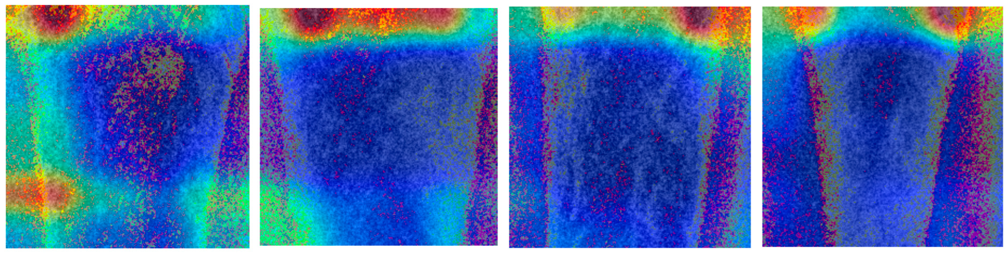
Experiments involving ablation with deep learning models demonstrated that expanding the input size to 122 × 122 did not enhance the results. This finding supports the use of relatively small ROIs, which can be attributed to the localized nature of the changes and the difficulty of isolating a single bone in the area as it grows. Additionally, the use of advanced augmentation techniques led to a decline in the outcomes. Since most augmentation methods alter pixel values, we avoided them in this study, as they cause undesirable changes in bone structure. We also investigated whether it is possible to determine which region the network uses for decision-making. However, a large variety of the determined regions (see Figure 5) did not allow for its use in further work.

We also need to emphasize that the age distribution of patients evaluated in these experiments is high, as they represent a cohort of patients from an orthopedic clinic. To minimize the influence of other medical conditions, we excluded patients with oncological diseases and fractures. We recognize that age-related diseases or medications may affect bone quality in these samples [29,30]. However, the study aimed to objectively assess bone quality by comparing it with chronological age. That was the reason for choosing X-rays in the first place. Moreover, in the case of forensic medicine, we do not have access to knowledge about a person’s medical history.

Our study supports the growing body of evidence that bone texture features can serve as reliable indicators for biological age estimation, extending the scope beyond traditional hand-based radiographs. Most existing models target pediatric populations using left-hand X-rays; however, our approach, based on pelvic X-rays (both CR and DR modalities), demonstrates that adult bone structures, especially in the pelvis, also encode discernible age-related patterns.

Using a texture-based feature analysis of 480 pelvic X-rays, we observed a maximum correlation around 0.5 between age and the ARM Theta 1 parameter, particularly in the femoral head (R05, L05). This suggests a significant correlation between trabecular architecture and chronological age. Our results are particularly relevant for adult and elderly populations, where traditional hand-based methods lose diagnostic value due to skeletal maturity. This directly addresses a limitation outlined by Manzoor Mughal et al. [2], who critically reviewed bone age assessment techniques and noted that the most widely used methods (e.g., Greulich–Pyle and Tanner–Whitehouse) become ineffective or ambiguous in adults. They highlighted the lack of standardized approaches for age estimation in skeletally mature individuals—an area where our pelvic X-ray analysis provides new potential.

Furthermore, our method offers interpretability, a feature that is increasingly lacking in modern AI-based systems. While black-box models, such as those presented by Deng et al. [31] and Chen et al. [32], leverage deep features from epiphyseal or articular regions, they often obscure the anatomical rationale behind their predictions. In contrast, our texture-parameter-based model, which focuses on clearly defined pelvic ROIs, enhances transparency and clinical relevance. This interpretability is particularly valuable in legal or forensic contexts, where decision accountability is essential—a concern raised by Satoh [1] in his discussion of bone age in medico-legal assessments.

Interestingly, Satoh [1] also emphasized the variation in bone maturation patterns across anatomical regions and patient backgrounds. Our findings echo this by demonstrating that ROI selection and preprocessing had differing effects on age correlation strength. Notably, we observed that narrowing the ROI to specific regions (e.g., R05, L05) significantly improved model performance.

These findings diverge from prevailing trends in the literature, where deep learning models are the dominant approach. For instance, Guo et al. [33] developed CNNs robust to real-world image noise in pediatric assessments, and Dallora et al. [34], in a comprehensive meta-analysis, confirmed the dominance of ML techniques—particularly in children. However, they also highlighted wide methodological variability and a gap in adult-specific models, reinforcing the importance of approaches like ours.

While separating by sex did not consistently increase correlation, focusing on key anatomical structures yielded more robust results. This supports the idea advanced by Deng et al. [31] that anatomical specificity in input data is crucial for improving bone age prediction, especially when using neural networks. Postmenopausal status may have influenced bone aging in females, but the change in bone quality that progresses with age is also observed in males [35].

In addition, our consistent identification of ARM Theta 1 as a top-performing feature aligns with the broader push toward texture-aware AI models. This may serve as a bridge between interpretable radiomic analysis and more opaque deep learning systems. Future work may involve combining these insights with CNN frameworks and activation map visualizations (e.g., Grad-CAM [36]), as proposed by Chen [33], to understand better which anatomical features drive model predictions.

Taken together, our findings demonstrate the viability of a texture-based pelvic radio–graph analysis as a complementary or alternative method for estimating adult bone age. They also underscore the need for anatomically diverse, age-inclusive datasets and hybrid modeling strategies that balance performance with interpretability. This not only meets clinical demands but also answers calls from the previous literature for reliable, transparent, and adult-focused bone age assessment frameworks (Manzoor Mughal et al. [2]; Satoh [1]). One of the criteria for selecting the type of endoprosthesis (short/long stem, cemented/cementless) for a given patient, apart from anatomical conditions, is the broadly understood bone quality [37,38]. Based on an assessment of plain radiograph Dorr’s classification which describes three types of proximal femoral geometry (Type A: narrow canal with thick cortical. Type B: moderate cortical walls. Type C: wide canal with thin cortical walls.) is not sufficient [39]. Dual energy X-ray absorptiometry (DXA) of the lumbar spine is not helpful in this case due to the potential presence of changes that could falsify the result [40]. Femoral neck densitometry may also be unreliable due to the presence of degenerative changes and secondary osteoporosis associated with unloading the affected limb [41]. It seems, therefore, that assessing bone age based on a pelvic X-ray in relation to the patient’s chronological age would be an invaluable tool in qualifying for alloplasty. All the more so because X-ray of the pelvis and hip joints is routinely performed as part of qualification for the procedure, comparing bone age with the patient’s chronological age, in addition to Bone Mineral Density (BMD) and Fracture Risk Assessment Tool (FRAX) approved by World Health Organization (WHO) [42], may also be helpful in the analysis of fracture risk assessment and may influence therapeutic decisions.

While the proposed AI model shows promising accuracy in bone age estimation, the mean absolute errors of 5–8 years must be interpreted with caution. In clinical scenarios involving borderline age cases, such discrepancies may lead to suboptimal decisions regarding treatment or implant selection. Therefore, the model should be viewed as a supportive tool, complementing—but not substituting—clinical expertise. Further development, including the use of larger datasets and model calibration for specific clinical contexts, is necessary to enhance reliability and reduce the risk of clinically meaningful misclassification. At this stage, this type of solution can only be a clue in forensic medicine.

Study [43] investigates the use of CT pubic bone scans as a method for age estimation in forensic anthropology, specifically within the Chinese population. A total of 468 CT scans from individuals aged 18 to 87 were analyzed to measure bilateral pubic BMD. The method demonstrated reasonable accuracy (MAE: 8.66 years for males, 7.69 for females), indicating its potential as a useful forensic tool. Similar results were obtained in [44], where mean absolute error of 12.1 for males and 10.8 for females was reported using CT images of pubic and ilium areas. These data were collected from post mortem computed tomography (PMCT) scans at the Tours Forensic Institute, comprising app. 20–80 age range.

4.1. Significance of the Study

The significance of our work lies in its contribution to the evolving landscape of radiographic age estimation, particularly for adult and aging populations. This domain has historically been underserved in both clinical and forensic practice. By shifting the focus from pediatric hand radiographs to pelvic bone structures, our study introduces a novel, anatomically relevant, and data-driven approach that captures microarchitectural changes associated with aging. This method is not only non-invasive and cost-effective but also leverages routinely acquired pelvic X-rays, making it highly applicable across various specialties, including orthopedics, geriatrics, endocrinology, and forensic medicine. The integration of texture-based radiomic analysis provides a transparent and interpretable alternative to “black-box” AI models, enabling more reliable clinical decision-making. Furthermore, the ability to estimate age from adult pelvic radiographs may support preoperative planning, risk stratification, assessment of bone health, and medico–legal evaluations. As such, our findings offer a practical and scalable tool that aligns with current trends in personalized and precision medicine.

4.2. Limitation of the Study

The collected dataset comprises patients from a single geographical region; therefore, it represents a unified cohort of Caucasian (European) origin. The number of samples is reasonable for traditional machine learning approaches; however, a larger number of samples could improve the results presented with deep learning models. The normal distribution of patients’ ages is natural for the population; however, it makes it challenging to estimate well samples from the range border.

A key limitation of the present study is the use of chronological age as the reference standard. While chronological age is a convenient and widely available label for AI training, it does not fully capture the biological state of the skeletal system. Ideal markers of bone aging would include bone mineral density, microarchitectural analysis, or other imaging-based indicators of bone quality that CAD AI-operated systems can capture. We acknowledge this limitation and view the current model as a step toward future approaches that integrate direct markers of skeletal health for more biologically relevant predictions based on image processing.

In our study, the regions of interest (ROIs) were manually annotated with the assistance of radiologists possessing a minimum of six years of experience in musculoskeletal imaging. While this ensured anatomical accuracy and clinical relevance, we acknowledge that the assessment of intra- and inter-observer variability was not performed quantitatively in this study.

However, to mitigate observer-dependent variation, we standardized the ROI selection protocol and used the same software tool (MaZda 19.02) under identical settings. Moreover, the choice of texture features was based on statistically robust correlations across the full dataset, followed by objective, automated machine learning and deep learning pipelines.

5. Conclusions

This work proposes a methodology for evaluating artificial intelligence methods in determining their applicability to medical data understanding. We present a pipeline that facilitates the easy evaluation of whether radiomic features are a reasonable means of describing pelvic radiographs and assessing patients’ ages. Initially, we suggest verifying whether there is a correlation between singular texture features and age. Since, in our case, the best scores showed a moderate correlation of almost 0.5, the experiments proceed with determination to see if it is possible to train a regression model. Firstly, traditional machine learning and deep learning models were evaluated based on uncorrelated features determined through statistical analysis. Here, the best models make a mistake of 5 or 9 years. The following experiments evaluated whether the automatic selection of the features is also promising. In those settings models made errors of 7 and 8 years, which show slight deterioration of outcomes, and high correspondence between the results. It is essential that by applying only CNN approaches, one can automatically determine the selection of the ROI.