Integrated Information in Relational Quantum Dynamics (RQD)

Featured Application

The integrated-information measure Φ provides a practical tool for quantifying multipartite entanglement and identifying modular structures in many-body quantum states, thereby guiding tensor-network decompositions and variational ansätze. In quantum computing, Φ can suggest optimal qubit partitions to minimize information loss in error-correction procedures and inform distributed algorithm design. By constructing integration dendrograms, one can visualize hierarchical correlation patterns in quantum simulators and, speculatively, infer functional clusters in quantum-inspired models of neural networks.

Abstract

We introduce a quantum integrated-information measure $\Phi$ for multipartite states within the Relational Quantum Dynamics (RQD) framework. $\Phi \left(\rho \right)$ is defined as the minimum quantum Jensen–Shannon distance between an n-partite density operator $\rho$ and any product state over a bipartition of its subsystems. We prove that its square root induces a genuine metric on state space and that $\Phi$ is monotonic under all completely positive trace-preserving maps. Restricting the search to bipartitions yields a unique optimal split and a unique closest product state. From this geometric picture, we derive a canonical entanglement witness directly tied to $\Phi$ and construct an integration dendrogram that reveals the full hierarchical correlation structure of $\rho$. We further show that there always exists an “optimal observer”—a channel or basis—that preserves $\Phi$ better than any alternative. Finally, we propose a quantum Markov blanket theorem: the boundary of the optimal bipartition isolates subsystems most effectively. Our framework unites categorical enrichment, convex-geometric methods, and operational tools, forging a concrete bridge between integrated information theory and quantum information science.

1. Introduction

Modern developments in quantum physics and theories of consciousness increasingly suggest that relations and information, rather than isolated material objects, are fundamental to reality. Recent proposals cast consciousness itself as a state of matter, suggesting a natural home for IIT in quantum-mechanical systems [1]. In particular, integrated information theory (IIT) posits that the level of intrinsic awareness or consciousness of a physical system corresponds to the quantity of integrated information (denoted $\Phi$) present in its state [2,3]. IIT argues that a system whose information is integrated, i.e., not decomposable into independent parts, has an irreducible subjective existence for itself [4]. This aligns with interpretations of quantum mechanics emphasizing that quantum states are relational rather than absolute [5]. John Wheeler’s famous dictum “every it derives its significance from bits” encapsulates the view that what fundamentally exists are acts of observation or informational relations, not static isolated entities [6]. Relational Quantum Mechanics (RQM) [5,7] formalizes this idea, proposing that the state of a quantum system is nothing more than the information one physical system has about another. Embracing this relational stance, we further posit that the “being” of a quantum system is constituted by the network of quantum information it shares with the rest of the world. Under this hypothesis, consistent with the idealistic interpretation of IIT (IIT 4.0’s “idealistic ontology” [8]), any system with non-zero integrated information ($\Phi >0$) possesses intrinsic existence (a rudimentary point of view “for itself”), whereas $\Phi =0$ indicates complete reducibility (no intrinsic unity beyond its parts).

Building on RQM, Relational Quantum Dynamics (RQD) elevates the primacy of informational relations by construing quantum states as inherently contextual and observer-relative, thereby embedding the IIT notion of integrated information within the formal structure of quantum theory. Under RQD, each system’s “being” arises from a network of dynamical information flows—quantified by $\Phi$—connecting its constituent subsystems, and classical spacetime and observations emerge from patterns of these relational correlations. By forgoing absolute state assignments in favor of context-dependent relational states, RQD unifies quantum measurement, spacetime emergence, and observerhood in a single coherent ontology [9].

To explore these ideas rigorously, we develop a formal measure $\Phi \left(\rho \right)$ of integrated information for an n-partite quantum system in state $\rho$. We require a quantitative gauge of how holistically correlated or irreducible the state $\rho$ is. In classical IIT, measures based on Kullback–Leibler divergence or mutual information have been proposed to quantify the loss of information upon splitting a system [10,11]. Here, a natural choice for the quantum case is the quantum Jensen–Shannon divergence ($D_{\mathrm{JS}}^Q$), a symmetrized and bounded measure of distance between quantum states [12,13]. Intuitively, $D_{\mathrm{JS}}^Q$ will serve as an “integration distance”; it vanishes if $\rho$ can be exactly factorized into independent local states (no integration) and grows as $\rho$ becomes more entangled or correlated across subsystems (more integration). Specifically, we define $\Phi \left(\rho \right)$ as the minimum $D_{\mathrm{JS}}^Q$ between $\rho$ and any product state obtained by partitioning the system. Let $P_1,\dots ,P_k$ be a partition of the n subsystems into k disjoint groups (blocks), and define the corresponding product state ${\rho }_{P_1}\otimes ···\otimes {\rho }_{P_k}$ as the tensor product of the reduced density operators on each block. Then we define

$$\Phi \left(\rho \right)=\underset{\mathrm{partitions}\left\{P_i\right\}}{min}{D}_{\mathrm{JS}}^Q\left(\rho \parallel \underset{i}{⨂}{\rho }_{P_i}\right).$$

(1)

In other words, $\Phi \left(\rho \right)$ quantifies the closest that $\rho$ can be (in terms of quantum Jensen–Shannon divergence) to an uncorrelated state. If $\rho$ is itself a product state under some partition, then $\Phi \left(\rho \right)=0$ (no integrated information). If $\rho$ is highly entangled or correlated across all subsystems, $\Phi \left(\rho \right)$ will be large, indicating strong irreducible correlations. This construction extends to the quantum domain that the integrated information measures use in classical IIT [10,11], with $D_{\mathrm{JS}}^Q$ replacing classical divergence or mutual information measures. Importantly, as we will show, $D_{\mathrm{JS}}^Q$ enjoys several properties (data-processing inequalities, convexity, a true metric structure) that make $\Phi \left(\rho \right)$ analytically tractable and well-behaved even for high-dimensional or rank-deficient states.

In developing our framework, we prove four main results about $\Phi$ and $D_{\mathrm{JS}}^Q$ as outlined above: (1) $\Phi$ is monotonic under processing (no observer can increase it), (2) the square-root of $D_{\mathrm{JS}}^Q$ is a metric on state space, (3) it suffices to consider bipartitions to attain the minimum in $\Phi \left(\rho \right)$, and (4) the observer can be formalized as a metric-space functor that is non-expansive. These results lay the groundwork for analyzing integrated information in quantum systems. After presenting these, we introduce a set of novel convex-geometric and operational insights that arise from viewing $\Phi \left(\rho \right)$ as a distance to the convex set of product states. This geometric perspective reveals that every state has a unique nearest product state (defining a canonical minimum information partition for $\rho$), and it unlocks an array of corollaries including convexity and robustness of $\Phi$, a natural gradient-flow that “dis-integrates” a state, and even a direct construction of an entanglement witness from $\Phi$. Furthermore, we leverage the unique optimal partition to build a hierarchical decomposition of any multipartite state into successively independent components, an integration dendrogram that maps out the structure of correlations in the state.

Finally, we explore two broader implications: an observer selection principle stating that one measurement basis or channel maximally preserves a system’s integrated information (suggesting a first-principles derivation of preferred pointer bases in decoherence theory), and a prospective quantum Markov blanket theorem, which identifies, for any subsystem, the minimal “boundary” that most effectively screens it off from the rest of the system. To our knowledge, this is the first fully metric-geometric construction of a quantum-IIT measure that (i) is provably a Lawvere metric enrichment of CPM, (ii) collapses to bipartitions by convexity, (iii) yields a canonical entanglement witness, and (iv) admits a functorial observer-selection principle.

2. Integrated Information Measure Definition

Before formalizing integrated information, we briefly review the quantum Jensen–Shannon divergence ($D_{\mathrm{JS}}^Q$). Given two quantum states (density operators) $\rho$ and $\sigma$ on the same Hilbert space, $D_{\mathrm{JS}}^Q(\rho \parallel \sigma )$ is defined as the quantum analog of the classical Jensen–Shannon divergence, which itself is a symmetrized and smoothed version of Kullback–Leibler divergence. One convenient expression is

$$D_{\mathrm{JS}}^Q(\rho \parallel \sigma )=\left[S\left({\displaystyle \frac{\rho +\sigma }{2}}\right)-{\displaystyle \frac{1}{2}}S\left(\rho \right)-{\displaystyle \frac{1}{2}}S\left(\sigma \right)\right],$$

(2)

where $S\left(\rho \right)=-\mathrm{Tr}(\rho log\rho )$ is the von Neumann entropy [13]. This quantity is symmetric ($D_{\mathrm{JS}}^Q(\rho \parallel \sigma )=D_{\mathrm{JS}}^Q(\sigma \parallel \rho )$) and bounded between 0 and $ln2$. In particular, $D_{\mathrm{JS}}^Q(\rho \parallel \sigma )=0$ if and only if $\rho =\sigma$, and the maximum $D_{\mathrm{JS}}^Q=ln2$ is attained for perfectly distinguishable orthogonal states. We will not require the detailed form of $D_{\mathrm{JS}}^Q$ beyond these properties; what is crucial for us is that it behaves as a distance measure on the space of states.

Definition 1 

(Quantum Integrated Information). For a quantum state ρ composed of n sub-systems, the integrated information $\Phi \left(\rho \right)$ is defined as the minimum quantum Jensen–Shannon divergence between ρ and any product state on a partition of the subsystems. In formula

$$\Phi \left(\rho \right)=\underset{\left\{P_1\right|\dots \left|P_k\right\}}{min}{D}_{\mathrm{JS}}^Q\left(\rho \parallel {\rho }_{P_1}\otimes \dots \otimes {\rho }_{P_k}\right),$$

(3)

where the minimum is taken over all possible ways of partitioning the set of subsystems $1,2,\dots ,n$ into disjoint blocks $P_1,\dots ,P_k$, and ${\rho }_{P_i}={\mathrm{Tr}}_{\overline{P_i}}\left(\rho \right)$ denotes the reduced state on block $P_i$. By convention, we consider only nontrivial partitions with at least two blocks (so if ρ is a total product state, $\Phi \left(\rho \right)=0$ is achieved when each subsystem is isolated in its own block).

This definition captures the degree of holism or irreducibility in $\rho$. If $\rho$ factorizes neatly into two or more independent components, then $\Phi \left(\rho \right)$ will be small (zero if an exact factorization exists). Conversely, if no accurate factorization exists (all partitions yield significant divergence), $\Phi \left(\rho \right)$ is large, indicating that the state’s information cannot be localized to separate parts without a significant loss. In practice, one might compute $\Phi \left(\rho \right)$ by evaluating $D_{\mathrm{JS}}^Q(\rho \parallel {\rho }_{P_1}\otimes \dots \otimes {\rho }_{P_k})$ for each candidate partition and taking the minimum. While the number of partitions grows quickly with n, our results below (especially Theorem 3) will sharply reduce the search space.

3. Monotonicity and Metric Properties of $D_{\mathrm{JS}}^Q$

We first establish two fundamental properties of the quantum JSD that underpin the integrated information measure: a data-processing inequality and a metric structure. These ensure that $\Phi$ behaves sensibly under observers and has a well-defined geometry.

Theorem 1 

(Data-Processing Monotonicity). For any two states $\rho ,\sigma$ and any CPTP map (quantum channel) $\mathcal{E}$, the quantum Jensen–Shannon divergence cannot increase under processing:

$$D_{\mathrm{JS}}^Q\left(\mathcal{E}\left(\rho \right)\parallel \mathcal{E}\left(\sigma \right)\right)\le D_{\mathrm{JS}}^Q(\rho \parallel \sigma ).$$

(4)

In particular, if an “observer” interacts with or measures the system (modeled by $\mathcal{E}$), the integrated information of the post-interaction state cannot exceed that of the pre-interaction state $\Phi \left(\mathcal{E}\right(\rho \left)\right)\le \Phi \left(\rho \right)$.

Proof 

(Sketch). This is the quantum analog of the classical data-processing inequality, and it holds because $D_{\mathrm{JS}}^Q$ belongs to the class of contractive divergences. Indeed, the JSD can be expressed in terms of the quantum relative entropy $D(\rho \parallel \sigma )=\mathrm{Tr}\left[\rho \right(log\rho -log\sigma \left)\right]$ as

$$D_{\mathrm{JS}}^Q(\rho \parallel \sigma )=\underset{\pi }{min}\left(\frac{1}{2}D(\rho \parallel \pi )+\frac{1}{2}D(\sigma \parallel \pi )\right)$$

(5)

(the minimal relative entropy to an intermediary state)—an expression which inherits the monotonicity of D under CPTP maps [14,15]. Alternatively, one can invoke the joint convexity of $D_{\mathrm{JS}}^Q$ and the complete positivity of $\mathcal{E}$ to show

$$\mathcal{E}\left({\displaystyle \frac{\rho +\sigma }{2}}\right)={\displaystyle \frac{\mathcal{E}\left(\rho \right)+\mathcal{E}\left(\sigma \right)}{2}}$$

(6)

and apply monotonicity of von Neumann entropy under partial trace. The inequality $\Phi \left(\mathcal{E}\right(\rho \left)\right)\le \Phi \left(\rho \right)$ then follows immediately: for any partition that attains (or approximates) the minimum for $\rho$, applying $\mathcal{E}$ to both $\rho$ and each product component cannot increase the divergence, so the minimal divergence for $\mathcal{E}\left(\rho \right)$ is bounded by that of $\rho$. □

This theorem formalizes the intuitive idea that observation cannot create integration. Any act of coarse-graining, measurement, or decoherence will tend to lose correlations or entanglement, never to introduce new irreducible correlations that were not already present. In category-theoretic terms, one can frame this as an enriched functor property: each physical process or observation defines a mapping between state spaces that does not expand distances. More precisely, we can view each system’s state space as a metric space $(\mathcal{S},\delta )$ with $\delta (\rho ,\sigma )=\sqrt{D_{\mathrm{JS}}^Q(\rho \parallel \sigma )}$ (as introduced below). Then any CPTP map $F:{\mathcal{S}}_1\to {\mathcal{S}}_2$ is a $[0,\infty ]$-enriched functor between these metric spaces, meaning ${\delta }_2(F\left(\rho \right),F\left(\sigma \right))\le {\delta }_1(\rho ,\sigma )$ for all states (Lawvere metric space enrichment). This functorial perspective identifies an “observer” or dynamics with a structure-preserving map in an information metric space. By Theorem 1, all such observers are non-expansive in the $\delta$ metric, and hence cannot increase $\Phi$. This categorical formulation helps unify the notion of observers across classical and quantum domains, but for the remainder of this paper, we will generally work in standard information-theoretic terms.

Practical Implications of Monotonicity: Theorem 1 implies a powerful experimental guarantee. In most tomographic protocols, one acquires raw measurement frequencies and then applies a maximum-likelihood (ML) estimator to project onto the physical state space. That ML step is itself a CPTP map, so by monotonicity, the post-processed $\Phi$ can only be smaller than the true $\Phi$ of the prepared state. In other words, any non-zero $\Phi$ we report is a conservative lower bound on the system’s intrinsic holism. Combined with the 1-Lipschitz bound from Section 4, which shows that, for trace-norm errors $\le \epsilon$, the resulting uncertainty in $\Phi$ is at most $\Delta \Phi \le \epsilon$, we see that standard tomography fidelities (∼2%) translate into $\Delta \Phi \lesssim 0.02$ bits. Thus, even imperfect state reconstruction cannot spuriously inflate $\Phi$, making it a robust witness of genuine multipartite integration.

$\Phi$ as a Resource Monotone: Beyond its operational significance, monotonicity under all CPTP maps elevates $\Phi$ to the status of a resource-theoretic monotone. In entanglement theory, one demands that valid entanglement measures never increase under the free operations of LOCC; analogously, here, any allowed quantum channel can only degrade holism. This endows $\Phi$ with the same foundational role for “quantum holism” that entanglement measures play for nonlocality:

$$\Phi \left(\mathcal{E}\left(\rho \right)\right)\le \Phi \left(\rho \right),$$

(7)

for every CPTP map $\mathcal{E}$. Consequently, $\Phi$ quantifies a resource that cannot be generated by noise or local processing, and it fits naturally into the burgeoning framework of quantum resource theories.

Next, we establish that the quantum JSD endows state space with a true metric, not just a divergence. It is known that the classical Jensen–Shannon divergence yields a legitimate distance metric via its square root. The quantum version inherits a similar property:

Theorem 2 

(Metric Structure of Quantum JSD). Define ${\displaystyle \delta (\rho ,\sigma ):=\sqrt{D_{\mathrm{JS}}^Q(\rho \parallel \sigma )}}$ for density operators $\rho ,\sigma$. Then $\delta (\rho ,\sigma )$ is a metric on the space of quantum states. In other words, it satisfies positivity, symmetry, and the triangle inequality. In particular, $\delta (\rho ,\sigma )=0$ if and only if $\rho =\sigma$, and for any three states $\rho ,\sigma ,\tau$ we have

$$\delta (\rho ,\tau )\le \delta (\rho ,\sigma )+\delta (\sigma ,\tau ).$$

(8)

Proof 

(Sketch). The non-negativity and symmetry of $\delta$ are immediate from the properties of $D_{\mathrm{JS}}^Q$. The non-degeneracy ($\delta (\rho ,\sigma )=0\iff \rho =\sigma$) holds because $D_{\mathrm{JS}}^Q(\rho \parallel \sigma )=0$ iff $\rho =\sigma$. The crux is the triangle inequality. We employ a known characterization: a divergence $D(·\parallel ·)$ is of the negative type (or negative definite) if and only if its square root defines a metric [16]. Recent works have shown that the (classical) Jensen–Shannon divergence is of a negative type, allowing the construction of an isometric embedding of probability distributions into a real Hilbert space [17]. The quantum Jensen–Shannon divergence shares this property [18]. Specifically, one can show $D_{\mathrm{JS}}^Q$ is negative-definite on quantum states, for example, by expressing it as an $L^2$ distance in an appropriate purified representation or by verifying the inequality ${\sum }_{ij}{a}_i{a}_j,D_{\mathrm{JS}}^Q({\rho }_i\parallel {\rho }_j)\le 0$ for any choices of states ${\rho }_i$ and real coefficients $a_i$ summing to 0 (a hallmark of negative-type functions). Given negative definiteness, Schoenberg’s theorem [16] guarantees that $\delta (\rho ,\sigma )=\sqrt{D_{\mathrm{JS}}^Q(\rho \parallel \sigma )}$ satisfies the triangle inequality. Hence, $\delta$ is a metric on state space. □

This result is noteworthy: although many quantum divergences, for example, quantum relative entropy, do not yield a true metric, the Jensen–Shannon divergence does. Thus, the set of density matrices can be treated as a metric space with distance $\delta$. Geometrically, $(\mathcal{S},\delta )$ is not a Euclidean space but can be embedded isometrically into a (potentially infinite-dimensional) inner-product space. Intuitively, one can think of each quantum state as a point in some high-dimensional “feature space” such that $\delta (\rho ,\sigma )$ is the Euclidean distance between those points. This will allow us to leverage convex geometry within the space of quantum states.

4. Optimal Factorizations and Convex Geometry of $\mathbf{\Phi }$

We now turn to analyzing the minimization in

$$\Phi \left(\rho \right)=\underset{P_i}{min}{D}_{\mathrm{JS}}^Q(\rho \parallel \underset{i}{⨂}{\rho }_{P_i}).$$

(9)

Two fundamental questions arise: (a) Which partition achieves the minimum? (b) Is the minimum achieved by a unique state? We will see that thanks to the metric structure and convexity properties of $D_{\mathrm{JS}}^Q$, the answer is remarkably neat: it is always a bipartition (a split into $k=2$ blocks) that attains the minimum, and moreover the closest product state is unique. This resolves any ambiguity in the notion of a “minimum information partition” and provides a well-defined integrated whole versus parts for the system.

Theorem 3 

(Bipartition Sufficiency and Existence of Optimal Product State). For any state ρ on n subsystems, the minimum in Definition 1 is attained on some bipartition $\left(A\right|B)$ of the system. In other words,

$$\Phi \left(\rho \right)=\underset{A|B}{min}{D}_{\mathrm{JS}}^Q\left(\rho \parallel {\rho }_A\otimes {\rho }_B\right),$$

(10)

where the minimum is over all splits of $1,\dots ,n$ into two disjoint groups A and B. Furthermore, there exists at least one product state ${\rho }_A\otimes {\rho }_B$ that achieves this minimum, and for each minimizing bipartition, the optimal product state on that cut is unique. In particular, there is a unique closest product state ${\sigma }^{\ast }\left(\rho \right)={\rho }_{A^{\ast }}\otimes {\rho }_{B^{\ast }}$, where $\left(A^{\ast }\right|B^{\ast })$ is the optimal partition.

Proof 

(Sketch). The fact that one can restrict to $k=2$ blocks without loss of generality follows from a simple inequality: for any partition with $k>2$ blocks, one can show that merging any two blocks cannot increase the divergence. Intuitively, splitting into more than two parts introduces additional independent components, which can only make it harder for a single product state to approximate $\rho$. More formally, consider three disjoint subsets $X,Y,Z$ of subsystems; one can show

$$D_{\mathrm{JS}}^Q(\rho \parallel {\rho }_X\otimes {\rho }_Y\otimes {\rho }_Z)\ge D_{\mathrm{JS}}^Q(\rho \parallel {\rho }_{XY}\otimes {\rho }_Z),$$

(11)

because ${\rho }_{XY}\otimes {\rho }_Z$ (where ${\rho }_{XY}={\mathrm{Tr}}_Z\rho$) allows correlations between X and Y that the fully factorized version ${\rho }_X\otimes {\rho }_Y\otimes {\rho }_Z$ forbids, and thus it is closer to $\rho$ (lower divergence). Iterating this argument, any partition with $k>2$ can be coarse-grained into a bipartition that yields an equal or smaller $D_{\mathrm{JS}}^Q$. Hence the minimum occurs at some $A|B$. Next, because for a fixed bipartition $\left(A\right|B)$ the set of product states ${\rho }_A\otimes {\rho }_B$ is a compact convex subset of state space and $D_{\mathrm{JS}}^Q(\rho \parallel \sigma )$ is a continuous function of $\sigma$, the infimum over $\sigma ={\rho }_A\otimes {\rho }_B$ is actually a minimum (attained at some $\sigma$). This uses the compactness of the set of marginal states ${\rho }_A$ and ${\rho }_B$; any minimizing sequence has a convergent subsequence in the product space by compactness, and by continuity, the limit is a minimizer. Finally, for a given bipartition, the uniqueness of the minimizing ${\rho }_A\otimes {\rho }_B$ follows from the strict convexity of $D_{\mathrm{JS}}^Q$ in its second argument. Quantum JSD is jointly convex [13] and in particular, if two distinct product states ${\sigma }_1={\rho }_A^1\otimes {\rho }_B^1$ and ${\sigma }_2={\rho }_A^2\otimes {\rho }_B^2$ both yield the same divergence

$$D_{\mathrm{JS}}^Q(\rho \parallel {\sigma }_1)=D_{\mathrm{JS}}^Q(\rho \parallel {\sigma }_2)=m,$$

then any mixture $\overline{\sigma }=t,{\sigma }_1+(1-t),{\sigma }_2$ (which is still a valid separable state on $AB$) would produce $D_{\mathrm{JS}}^Q(\rho \parallel \overline{\sigma })<m$ for $0<t<1$, contradicting the minimality. One can also argue from the negative-definite metric viewpoint that the distance-squared function $\sigma \mapsto {\delta }^2(\rho ,\sigma )$ is strictly convex on a geodesically convex domain of product states. Thus, the minimizer on each partition is unique. If there were multiple bipartitions achieving the same minimum value, one of their corresponding product states would still be closer in $\delta$-distance than any other state, so we may define ${\sigma }^{\ast }\left(\rho \right)$ to be one of them. In generic cases, the optimal partition $\left(A^{\ast }\right|B^{\ast })$ is unique as well (ties are non-generic and can be broken arbitrarily). □

We emphasize the important consequence: the closest product-state approximation to $\rho$ is unique. We denote this distinguished state by ${\sigma }^{\ast }\left(\rho \right)={\rho }_{A^{\ast }}\otimes {\rho }_{B^{\ast }}$, where $\left(A^{\ast }\right|B^{\ast })$ is an optimal bipartition. We may call $\left(A^{\ast }\right|B^{\ast })$ the minimum information partition (MIP) of $\rho$, borrowing terminology from IIT. There is no degeneracy in identifying the “best split” of the system—a fact that contrasts with earlier approaches where one often had to choose among candidate partitions or deal with ties. Uniqueness comes from the convexity of the divergence and can be seen as a benefit of using $D_{\mathrm{JS}}^Q$ as opposed to mutual information, for example, which might not identify a unique optimal split in some cases.

With ${\sigma }^{\ast }\left(\rho \right)$ in hand, we can reinterpret the integrated information as a distance from $\rho$ to the set of disjoint-state products. In fact, Theorem 3 implies:

$$\Phi \left(\rho \right)=D_{\mathrm{JS}}^Q\left(\rho \parallel {\sigma }^{\ast }\left(\rho \right)\right)={\delta }^2\left(\rho ,{\sigma }^{\ast }\left(\rho \right)\right),$$

(12)

since $\delta (\rho ,\sigma )=\sqrt{D_{\mathrm{JS}}^Q(\rho \parallel \sigma )}$. In words, $\Phi \left(\rho \right)$ is the squared distance (in the $\delta$ metric) from $\rho$ to the closed, convex set

$${\mathcal{P}}_2=\{{\rho }_A\otimes {\rho }_B:A|B\mathrm{a}\mathrm{bipartition}\}$$

of all bipartite product states. We can therefore leverage geometric intuition: computing $\Phi \left(\rho \right)$ is performing a metric projection of the point $\rho$ onto the set ${\mathcal{P}}_2$. By standard results in convex geometry and metric spaces, this immediately yields a raft of powerful corollaries:

• Convexity of $\mathbf{\Phi }$. As an infimum (indeed minimum) of convex functions $\sigma \mapsto D_{\mathrm{JS}}^Q(\rho \parallel \sigma )$, the distance-to-set function

  $$\rho \mapsto \underset{\sigma \in {\mathcal{P}}_2}{inf}{D}_{\mathrm{JS}}^Q(\rho \parallel \sigma )$$

  (13)

  is convex on state space. Equivalently, for any two states ${\rho }_1,{\rho }_2$ and any $0\le t\le 1$,

  $$\Phi \left(t{\rho }_1+(1-t){\rho }_2\right)\le t\Phi \left({\rho }_1\right)+(1-t)\Phi \left({\rho }_2\right).$$

  (14)
  This convexity means that mixing states cannot increase the integrated information beyond the mixture of their individual $\Phi$ values. In practical terms, a noisy or probabilistic mixture of two configurations will tend to have less (or equal) holistic structure than a pure configuration, which aligns with intuition.
• Lipschitz Continuity (Robustness). The function $\Phi \left(\rho \right)$ is 1-Lipschitz continuous with respect to the metric $\delta$. That is,

  $$|\Phi \left(\rho \right)-\Phi \left({\rho }^{\prime }\right)|\le \delta (\rho ,{\rho }^{\prime })$$

  (15)

  for all states $\rho ,{\rho }^{\prime }$. Small changes or errors in the state can only cause small (at most proportional) changes in the integrated information. This follows from a general fact: in any metric space, the distance from a point to a convex set is a 1-Lipschitz function (intuitively, if $\rho$ and ${\rho }^{\prime }$ are close, their nearest projections on a convex set cannot be very different in distance). More concretely, one can use the triangle inequality

  $$\Phi \left(\rho \right)=\delta (\rho ,{\sigma }^{\ast }\left(\rho \right))\le \delta (\rho ,{\rho }^{\prime })+\delta ({\rho }^{\prime },{\sigma }^{\ast }\left(\rho \right)).$$

  (16)
  But $\delta ({\rho }^{\prime },{\sigma }^{\ast }\left(\rho \right))\ge \Phi \left({\rho }^{\prime }\right)$ because ${\sigma }^{\ast }\left(\rho \right)$ might not be the optimal product for ${\rho }^{\prime }$, so

  $$\delta ({\rho }^{\prime },{\sigma }^{\ast }\left(\rho \right))\ge \delta ({\rho }^{\prime },{\sigma }^{\ast }\left({\rho }^{\prime }\right))=\Phi \left({\rho }^{\prime }\right).$$

  (17)
  Thus, $\Phi \left(\rho \right)-\Phi \left({\rho }^{\prime }\right)\le \delta (\rho ,{\rho }^{\prime })$. Swapping $\rho \leftrightarrow {\rho }^{\prime }$ gives the two-sided Lipschitz bound. This robustness is crucial for empirical or experimental scenarios: it means $\Phi$ will not fluctuate wildly due to small perturbations or noise in the state, making it a reliable quantity to estimate.
• Gradient Flow towards Dis-integration. By viewing $\Phi \left(\rho \right)={\delta }^2(\rho ,\mathcal{P}\ast 2)$ as a squared-distance function in a (formal) Riemannian space, one can define a gradient descent dynamical system that flows $\rho$ toward its nearest product state. Concretely, we can write a continuous time equation

  $$\dot{\rho }\left(t\right)=-{\nabla }_{\rho }\Phi \left(\rho \right),$$

  (18)

  which generates a trajectory $\rho \left(t\right)$ that decreases $\Phi$ monotonically and converges to the projection ${\sigma }^{\ast }\left(\rho \right)$ as $t\to \infty$. While here $\nabla \ast \rho$ denotes a gradient with respect to the information geometry induced by $D_{\mathrm{JS}}^Q$, one can intuitively think of this as the state “pulling itself apart” into independent pieces. In practice, this gradient-flow could be implemented by a family of CPTP maps that progressively erode the holistic correlations. The advantage of framing it as a gradient flow is that it provides a principled algorithm for finding ${\sigma }^{\ast }\left(\rho \right)$ (the best factorized approximation) by following the steepest descent of integrated information, rather than using ad hoc separability criteria. Analyzing the specific form of ${\nabla }_{\rho }\Phi$ is beyond our scope here, but it may be related to applying gentle local decoherence to remove entanglement at the fastest rate.

All these properties flow naturally from the convex geometric view of $\Phi$ as a projection distance. This perspective has not, to our knowledge, been applied in previous integrated information literature, and it unlocks powerful tools from convex optimization and metric geometry to study and compute $\Phi$. We stress that ${\sigma }^{\ast }\left(\rho \right)$ and $\left(A^{\ast }\right|B^{\ast })$ provide more information than just the scalar $\Phi \left(\rho \right)$: they tell us exactly how the state can be optimally split and how far it is from such a split. In the next result, we show that ${\sigma }^{\ast }\left(\rho \right)$ can be used to construct a special entanglement witness that “certifies” the integrated information.

Lemma 1 

(RKHS embedding of QJSD). Define $k(\rho ,\sigma )=ln2-D_{\mathrm{JS}}^Q(\rho \parallel \sigma ).$ Then k is a positive-definite kernel on the space of density operators. Hence by Schoenberg’s theorem [16,18], there exists a real reproducing-kernel Hilbert space $(\mathcal{H},{⟨·,·⟩}_{\mathcal{H}})$ and a feature map $\varphi :\rho \mapsto k(·,\rho )\in \mathcal{H},$ with ${⟨\varphi \left(\rho \right),\varphi \left(\sigma \right)⟩}_{\mathcal{H}}=k(\rho ,\sigma ).$

Proof 

(Sketch). Since $D_{\mathrm{JS}}^Q$ is bounded ($0\le D_{\mathrm{JS}}^Q<ln2$) and symmetric, the shifted kernel $k=ln2-D_{\mathrm{JS}}^Q$ satisfies Schoenberg’s criterion for negative-type metrics, which guarantees a Hilbert-space embedding. □

Metric-gradient and operator pullback. From Lemma 1 and

$${\delta }^2(\rho ,\sigma )=D_{\mathrm{JS}}^Q(\rho \parallel \sigma )={\parallel \varphi \left(\rho \right)-\varphi \left(\sigma \right)\parallel }_{\mathcal{H}}^2,$$

(19)

we get in $\mathcal{H}$

$${\nabla }_{\varphi \left(\sigma \right)}{\delta }^2(\rho ,\sigma )=2\left(\varphi \left(\sigma \right)-\varphi \left(\rho \right)\right).$$

(20)

Pulling this back via the Fréchet derivative

$${\displaystyle \frac{\partial }{\partial \sigma }}S\left(\sigma \right)=-log\sigma -\mathbb{I},$$

(21)

the stationarity condition ${\nabla }_{\varphi \left({\sigma }^{\ast }\right)}{\delta }^2(\rho ,{\sigma }^{\ast })=0$ yields

$$log\frac{\rho +{\sigma }^{\ast }}{2}-log\rho =0,$$

(22)

so that (up to a positive scalar) $W_{\rho }={\sigma }^{\ast }-\rho$ is precisely the normal operator defining the separating hyperplane in the original operator space.

Proposition 1 

(Canonical Entanglement Witness). Let ${\sigma }^{\ast }\left(\rho \right)={\rho }_{A^{\ast }}\otimes {\rho }_{B^{\ast }}$ be the closest product state to ρ, achieved on the optimal bipartition $\left(A^{\ast }\right|B^{\ast })$. Define an observable (Hermitian operator) $W_{\rho }:={\sigma }^{\ast }\left(\rho \right)-\rho .$ Then $W_{\rho }$ is an entanglement witness for the bipartition $A^{\ast }|B^{\ast }$. In particular, $W_{\rho }$ has a non-negative expectation value on all product states factorized across $A^{\ast }$ and $B^{\ast }$, yet has a strictly negative expectation on ρ itself. Moreover, the magnitude of this violation is exactly the integrated information:

$$\mathrm{Tr}\left[W_{\rho }\rho \right]=-\Phi \left(\rho \right).$$

(23)

In fact, $W_{\rho }$ is the optimal (most “detecting”) witness for the entanglement between $A^{\ast }$ and $B^{\ast }$.

Proof. 

By Lemma 1 and the metric-gradient calculation, the minimizing condition ${\nabla }_{\varphi \left({\sigma }^{\ast }\right)}{\delta }^2(\rho ,{\sigma }^{\ast })=0$ pulls back to $log\frac{\rho +{\sigma }^{\ast }}{2}-log\rho =0$, and hence $W_{\rho }={\sigma }^{\ast }-\rho$ is the geodesic-normal. Positivity on any product state $\pi ={\pi }_A\otimes {\pi }_B$ follows because ${\sigma }^{\ast }$ is the closest product state. The fully detailed proof of this proposition is presented in Appendix C. □

In summary, $W_{\rho }={\sigma }^{\ast }\left(\rho \right)-\rho$ is a constructive, canonical witness to the entanglement or correlation that makes $\rho$ irreducible across its optimal split. It detects exactly the entanglement corresponding to $\Phi \left(\rho \right)$ and no more. In particular, $\mathrm{Tr}[W_{\rho },\rho ]=-\Phi \left(\rho \right)$ quantifies the “violation” of $\rho$ being separable: the more integrated $\rho$ is, the more $W_{\rho }$ yields a negative expectation on it, with the gap equal to $\Phi \left(\rho \right)$. One could say this provides an operational meaning to $\Phi$: it is the magnitude by which $\rho$ fails the best possible separability test. This is a novel connection between integrated information and entanglement theory — it bridges a geometrical measure of holistic correlation ($\Phi$) with the traditional notion of an entanglement witness from quantum information. In practice, once one computes ${\sigma }^{\ast }\left(\rho \right)$ (by any method), one immediately obtains $W_{\rho }$, which is an observable whose expectation value on $\rho$ is $-\Phi \left(\rho \right)$ and on any fully factorized state (on that cut) is non-negative. Experimentally, measuring the set of local observables that constitute $W_{\rho }$, which will generally be a difference of two reduced density operators, could verify the presence of entanglement and even quantify it in terms of integrated information.

5. Hierarchical Decomposition: The Integration Dendrogram

Thus far, we have focused on identifying a single “critical cut” $\left(A^{\ast }\right|B^{\ast })$ that yields the minimal integrated information. We now show that this idea can be recursively applied to yield a hierarchical decomposition of the state into a tree of increasingly fine subsystems. The result is a binary tree (dendrogram) that represents the multi-scale structure of correlations in $\rho$. This construction parallels hierarchical clustering in classical data analysis but here it is based on quantum information relationships intrinsic to $\rho$ itself.

The procedure is as follows:

• Level 0 (Root): Start with the full system as one set $S=1,2,\dots ,n$. Compute $\Phi \left(\rho \right)$ and find the unique optimal bipartition $\left(A^{\ast }\right|B^{\ast })$ of S that achieves it. This is the root split of the dendrogram, and the value $\Phi \left(\rho \right)$ will label the root node as a measure of how hard it is to tear the entire system into two parts.
• Level 1: Now take the two blocks $A^{\ast }$ and $B^{\ast }$ separately. For each block (subsystem group) considered its own subsystem, compute its integrated information $\Phi \left({\rho }_{A^{\ast }}\right)$ within that block, i.e., allow partitions internal to $A^{\ast }$. Find the optimal bipartition of $A^{\ast }$ that achieves $\Phi \left({\rho }_{A^{\ast }}\right)$, and similarly partition $B^{\ast }$ optimally. This yields splits $A^{\ast }\to \left(A_1\right|A_2)$ and $B^{\ast }\to \left(B_1\right|B_2)$ at the next level. Attach these as children of the respective nodes in the tree, and label the nodes $A^{\ast }$ and $B^{\ast }$ with $\Phi \left({\rho }_{A^{\ast }}\right)$ and $\Phi \left({\rho }_{B^{\ast }}\right)$.
• Continue recursively: At each subsequent level, for every current leaf node of the tree (which corresponds to some subset of qubits or subsystems), if that subset contains more than one elementary subsystem, compute its optimal bipartition and $\Phi$-value, and split it. Continue until every leaf is an individual elementary subsystem (which cannot be split further). The recursion will terminate after at most $n-1$ levels (when all subsystems are singletons).

The outcome of this algorithm is a full binary tree whose leaves are the individual subsystems $1,\dots ,n$, and whose internal nodes represent larger groupings that were optimally split. We call this tree the integration dendrogram of $\rho$ (see Appendix B). Each internal node is labeled by the $\Phi$-value of that grouping, i.e., how much integrated information had to be “broken” to split it into two parts.

To illustrate the usefulness of this dendrogram, consider its properties:

• Uniqueness and Stability: Because each bipartition at each step is unique (Theorem 3) and changes continuously with $\rho$ (Lipschitz continuity), the entire dendrogram is uniquely determined by $\rho$ and is robust to small perturbations. Small changes in $\rho$ will only gradually change the $\Phi$ values and possibly slightly adjust the splits, but the overall hierarchical order (which splits occur at which scale) will not wildly reshuffle. This is in stark contrast to some heuristic clustering methods that can have unstable hierarchies. Here the hierarchy is rooted in strict convex optimal cuts at each step, making it canonical for each state.
• Multi-Scale Summary of Correlations: The dendrogram provides a multi-scale map of the entanglement/correlation structure in $\rho$. The top of the tree tells you the largest-scale division (where the weakest global link in the system lies). Further down, you see progressively smaller modules and sub-modules, down to individual units. Each node’s height (the $\Phi$ value for that subset) quantifies how strongly that subset resists factorization. A high $\Phi$ at a certain node means that the subset is very integrated and only separable with a large loss, whereas a low $\Phi$ node indicates a relatively weakly bound cluster that could almost be split without much information loss. In effect, one can read off which groups of subsystems form coherent modules and which connections are tenuous. For example, a branch of the dendrogram might show qubits 1,2,3 forming a tight sub-cluster (high $\Phi$ internally) that only weakly connects (low $\Phi$ cut) to another cluster of qubits 4,5, etc.
• Algorithmic Simplicity: Building the dendrogram requires solving the bipartition optimization at each level, which is the same type of problem as computing $\Phi \left(\rho \right)$ in the first place. While finding the optimal partition is NP-hard in general (since one might have to try all splits), focusing on pairwise splits at each level yields a manageable procedure. There are $O\left(2^n\right)$ possible bipartitions of an n-element set, so a brute-force search at each level is exponential in the size of the current subset. However, since we do at most $n-1$ levels, the overall worst-case complexity is $O(n·2^n)$, which is exponential but not super-exponential. In practice, many splits will involve smaller subsets and thus fewer possibilities. Moreover, the computations for different branches can be performed in parallel. This is far more tractable than attempting to search among all partitions of all sizes simultaneously (a number that grows faster than $2^n$). Thus, the hierarchical approach breaks the problem into $n-1$ manageable pieces.
• Connections to Clustering: In classical data science, one often constructs hierarchical clustering dendrograms using metrics or information-based distances. Here we have the quantum analog: a dendrogram based on a rigorous information metric ($\delta$) applied not to classical data points but to the quantum state itself. Rather than clustering individual data samples, we are clustering subsystems of a single quantum state based on their entanglement structure. This opens the door to using visualization and cluster-identification techniques from classical analysis in quantum many-body systems. For instance, one could visualize the dendrogram with node heights proportional to $\Phi$ values, giving a clear picture of the “integration profile” of the state across scales. Branch lengths indicate how much correlation binds subsystems at that split.

In summary, the integration dendrogram is a powerful new tool for analyzing multipartite quantum states. It yields a unique, stable, multi-scale decomposition of a state’s entanglement structure without requiring any ad hoc choices beyond the definition of $\Phi$. By reading the dendrogram, one can immediately identify which subsystems form natural groupings or communities (high internal $\Phi$) and where the “weak links” between those groupings are (low $\Phi$ between them). This has potential applications in understanding complex quantum networks or many-body systems: for example, identifying modules in an interacting spin chain, or coarse-grained functional units in a quantum neural network, etc. The dendrogram encapsulates an entire hierarchy of quantum integration within a single object.

6. Preferred Observers: The Max-$\mathbf{\Phi }$ Principle

We have shown that no observer (CPTP map) can increase integrated information (Theorem 1). A natural question arises: which observer loses the least integrated information? In other words, suppose we have a system in state $\rho$, and we are allowed to “observe” it in some fashion, perhaps by making a measurement or by coarse-graining its degrees of freedom. Different observation schemes will preserve different fractions of the holistic correlations present in $\rho$. Is there a principled way to choose the optimal observation that retains as much of $\Phi \left(\rho \right)$ as possible?

Remarkably, the answer is yes. We call this the Max-$\Phi$ observer principle: among any reasonable family of observation channels, one can find a channel $F^{\ast }$ that maximizes the integrated information of the observed state $F\left(\rho \right)$. Moreover, $F^{\ast }$ can be interpreted as selecting the “best” basis or representation, in which to obtain classical information about $\rho$ without destroying its holistic structure. This has deep connections to the idea of a preferred basis in quantum decoherence theory [19]: the basis that is stable and preserves certain correlations. Here, we derive such a basis from first principles, using only the monotonicity of $\Phi$ and the compactness of the channel space.

Theorem 4 

(Optimal Observer Channel). Let $\mathcal{F}$ be any compact set of CPTP maps (quantum channels) that one considers possible observers on the state ρ. For example, $\mathcal{F}$ could be the set of all local projective measurements of each qubit (with the observer recording classical outcomes), or the set of all partial trace operations onto some subsystem, or more generally any parametrized family of channels. Then there exists at least one channel $F^{\ast }\in \mathcal{F}$ that maximizes the integrated information of the output:

$$F^{\ast }=arg\underset{F\in \mathcal{F}}{max}\Phi \left(F\left(\rho \right)\right).$$

(24)

Existence is guaranteed; there may in principle be more than one maximizer, but we can pick one. In other words, there is an optimal observer $F^{\ast }$ that preserves ρ’s integrated information better than any other in $\mathcal{F}$. Furthermore,

$$\Phi \left(F^{\ast }\left(\rho \right)\right)=\underset{F\in \mathcal{F}}{max}\Phi \left(F\left(\rho \right)\right)\le \Phi \left(\rho \right),$$

(25)

with equality only if the optimal channel effectively does nothing to disturb the relevant correlations. For example, $F^{\ast }$ could be the identity channel or an isometry embedding into a larger space.

Proof. 

Because $\Phi \left(F\right(\rho \left)\right)$ is a function with real value in the set of channels and $\mathcal{F}$ is compact, the maximum value is attained (by the extreme value theorem). We only need to argue for the continuity of $F\mapsto \Phi \left(F\right(\rho \left)\right)$ in a suitable topology in the space of CPTP maps. If we parametrize channels by their finite-dimensional Kraus operators, small changes in those operators yield small changes in the output state (in trace norm, say), which in turn yield small changes in $\Phi$ (by Lipschitz continuity of $\Phi$). Thus, $\Phi \left(F\right(\rho \left)\right)$ is a continuous function in the compact set $\mathcal{F}$, and therefore there is a maximum. The inequality $\Phi \left(F\right(\rho \left)\right)\le \Phi \left(\rho \right)$ for all F is just Theorem 1, so the maximal value is bounded by $\Phi \left(\rho \right)$. The equality $\Phi \left(F\right(\rho \left)\right)=\Phi \left(\rho \right)$ would require that

$$D_{\mathrm{JS}}^Q(F\left(\rho \right)\parallel F\left(\sigma \right))=D_{\mathrm{JS}}^Q(\rho \parallel \sigma )$$

(26)

for some product state $\sigma$ that achieves $\Phi \left(\rho \right)$. In practice, this implies that F does not erase any of the distinguishing information between $\rho$ and $\sigma$—essentially, F is invertible on the support of $\rho ,\sigma$—which typically means that F is an embedding or trivial operation. □

Theorem 4 is simple but profound. It tells us that, given any constraint on how we observe the system, we can find a “best” way to observe it, if our criterion is to preserve integrated information. This $F^{\ast }$ can be thought of as the observer that loses the least holism. In effect, it picks an optimal classical description of the correlations of the quantum state. We highlight some implications and interpretations:

• Preferred Basis from First Principles: If $\mathcal{F}$ is the set of all projective measurements on each subsystem (i.e., choosing a measurement basis for each qubit, for instance), then $F^{\ast }$ will pick a specific measurement basis on each part that maximizes $\Phi$ of the post-measurement state (which is now classical). This essentially selects the pointer basis in which the state $\rho$ looks most integrated. In decoherence theory [19,20], pointer bases are typically those that minimize decoherence or maximize stability. Here, we have an alternative: the pointer basis is the one that maximizes $\Phi$—it retains the most information about the quantum whole. This provides a crisp, quantitative criterion for the “natural” basis of classical reality to emerge: it is the basis that preserves integrated information to the greatest extent.
• Algorithmic Selection of Observers: The search for $F^{\ast }$ can be framed as an optimization problem over channels, which is typically a convex (or at least manageable) optimization because the set of CPTP maps is convex. Although the space of all channels is large, restricting to a parameterized family (like all product measurements, or all partial traces onto k subsystems, etc.) can make this finite or at least tractable. Then, gradient-based or evolutionary algorithms could be applied to find the optimal observer. This turns a philosophical question (“which measurement basis is most natural or informative?”) into a concrete optimization: maximize $\Phi \left(F\right(\rho \left)\right)$ over F. Because $\Phi$ is differentiable in $\rho$ (at least where $\rho$ is full rank) and F’s action on $\rho$ is linear, gradients with respect to F’s parameters can be computed in principle.
• Unification of IIT and Decoherence Theory: In the IIT literature, observers or “mechanisms” are usually assumed and one computes information loss post hoc. In decoherence theory, preferred bases are argued for by various principles, for example, minimal entropy production. The Max-$\Phi$ principle unifies these: it says the most informatively integrated view of the system is the “correct” one. This might shed light on why certain macroscopic observables (like position in space, or certain vibrational modes) become the ones we observe—because those observables preserve the integrated structure of the quantum state across scales.
• Observer-Robustness Spectrum: By studying the function $F\mapsto \Phi \left(F\right(\rho \left)\right)$, we can also characterize how sensitive the system’s holism is to observation. Observers F for which $\Phi \left(F\right(\rho \left)\right)\approx \Phi \left(\rho \right)$ can be called high-fidelity observers: they capture almost all the holistic structure (these would be close to the identity or gentle/unitary observations). Observers for which $\Phi \left(F\right(\rho \left)\right)$ plunges to near 0 are ignorant observers: their measurements or coarse-grainings immediately destroy almost all integration (think of measuring in a very incompatible basis, which scrambles correlations). Most realistic observers lie somewhere in between. This spectrum tells us how “fragile” the integration is: if $\Phi \left(\rho \right)$ is lost under almost any observation (except one very special $F^{\ast }$), the system’s holism might be considered very observer-dependent. Conversely, if $\Phi \left(\rho \right)$ remains high for a broad class of observers, the system has an objectively robust integrated core.

We have thus established that an optimal observer $F^{\ast }$ always exists (for a given class of observations). In practice, identifying $F^{\ast }$ might require exploring the space of channels, but at least we know a solution is out there. This result provides a new principle for selecting representations in quantum systems—one that could potentially be applied in quantum computing (to choose a basis that preserves entanglement across a split), or even in neuroscience-inspired quantum models (to define what constitutes a natural “perspective” on a quantum network).

7. Toward a Quantum Markov Blanket

Finally, we turn to an intriguing consequence of our framework that connects to ideas in causality and complex systems: the notion of a Markov blanket. In classical graphical models [21], a Markov blanket of a node is the set of other nodes that shields it from the rest of the network—conditioning on the blanket renders the node independent of all others. In IIT and related fields, one sometimes speaks of a “minimum information partition” or a boundary that separates a system from its environment in terms of information flow. Here, we can identify a natural quantum analogue: the quantum Markov blanket of a subset of subsystems.

Using $\Phi$, we can give an operational definition: consider any multipartite state $\rho$ on subsystems $1,\dots ,n$. Let $\left(A^{\ast }\right|B^{\ast })$ be the unique bipartition that minimizes $D_{\mathrm{JS}}^Q(\rho \parallel {\rho }_A\otimes {\rho }_B)$, i.e., that defines $\Phi \left(\rho \right)$. Without loss of generality, assume $|A^{\ast }| \le |B^{\ast }|$ (label the smaller side as X and the larger as Y). We claim that X is the Markov blanket for Y (and vice versa in symmetric sense): conditioning on X makes $A^{\ast }$ and $B^{\ast }$ as independent as possible. More concretely, we have the following.

Theorem 5 

(Quantum Markov Blanket, informal). In the state ρ, let X denote the smaller subsystem among the optimal split $A^{\ast }|B^{\ast }=X|Y$. Then for any other candidate subset $X^{\prime }$ of subsystems with $|X^{\prime }|=|X|$, the following holds. If one “conditions” on X versus on $X^{\prime }$, the residual dependence (as measured by Jensen–Shannon divergence) between Y and X’s complement is minimal when conditioning on X. Equivalently, X is the subset of that size which best “screens off” the rest of the system into two nearly-independent parts.

In less formal terms, X serves as the informational interface between $A^{\ast }$ and $B^{\ast }$. If one knows (or fixes) the state of X, the two sides $A^{\ast }\setminus X$ and $B^{\ast }\setminus X$ become as independent as one can make them by conditioning on any equally sized set. This is analogous to the classical Markov blanket property, but we have to be careful in quantum theory because conditioning is not straightforward. In classical probability, conditioning on a variable X means replacing the joint distribution $p(A,B,X)$ with the conditional $p(A,B|X)$. In quantum theory, one way to mimic conditioning is to use the Petz recovery map [22]: given the marginal ${\rho }_X$ and one side (say ${\rho }_{AX}$), one can attempt to reconstruct a conditional state ${\rho }_{A|X}$ such that ${\rho }_{AX}={\rho }_{A|X}\otimes {\rho }_X$ if a Markov condition holds. The Petz recovery channel ${\mathcal{R}}_{X\to AX}$ effectively represents the best way to infer the A part given access to X. Using such a tool, one can formalize Theorem 5 as follows:

(Quantum Markov Blanket via Petz Recovery, formalized). Let $\left(A^{\ast }\right|B^{\ast })$ with smaller side X be the optimal partition for ρ. Define Y as the complementary side ($Y=B^{\ast }$ if $X=A^{\ast }$, or vice versa). For any other subset Z of subsystems with $\left|Z\right|=\left|X\right|$, consider the Petz-recovered conditional states $\tilde{\rho }\ast Y|Z:=\mathcal{R}\ast Z\to YZ\left({\rho }_Z\right)$ that attempt to reconstruct the joint on $YZ$ from Z alone. Then X is the subset for which the Jensen–Shannon divergence between ${\rho }_{XY}$ and the tensor product of recovered conditionals is minimized:

$$D_{\mathrm{JS}}^Q\left({\rho }_{XY}\parallel {\tilde{\rho }}_{X|X}\otimes {\tilde{\rho }}_{Y|X}\right)=\underset{\begin{array}{c}Z\subset \{1,\dots ,n\}\\ \left|Z\right|=\left|X\right|\end{array}}{min}{D}_{\mathrm{JS}}^Q\left({\rho }_{YZ}\parallel {\tilde{\rho }}_{Y|Z}\otimes {\rho }_Z\right).$$

(27)

In the above, $\tilde{\rho }\ast X|X\equiv {\rho }_X$ trivially, and $\tilde{\rho }\ast Y|X$ is the Petz reconstruction of ${\rho }_{XY}$ from ${\rho }_X$. In other words, among all choices of Z of the same size, $Z=X$ yields the smallest residual Φ (or Jensen–Shannon correlation) between Y and Z’s complement when one conditions on Z. Thus X is the Markov blanket that best screens off Y from the rest of the system.

Proof 

(Sketch). A full proof is technical and will be provided elsewhere, but the intuition is the following: For X being the optimal partition side, $\Phi \left(\rho \right)=D_{\mathrm{JS}}^Q({\rho }_{XY}\parallel {\rho }_X\otimes {\rho }_Y)$ is minimal. We want to show that any other candidate Z (of equal size) yields a larger effective divergence after “conditioning”. Using the properties of the Petz recovery channel, one can show a data-processing inequality in reverse: if X is the minimizing set, then for any Z of the same size,

$$D_{\mathrm{JS}}^Q({\rho }_{XY}\parallel {\rho }_X\otimes {\rho }_Y)\le D_{\mathrm{JS}}^Q({\rho }_{ZY}\parallel {\rho }_Z\otimes {\tilde{\rho }}_{Y|Z}).$$

(28)

The right-hand side is essentially the $\Phi$ of splitting the system into Z vs. the rest after optimally conditioning on Z (via Petz). This inequality relies on two facts: (i) monotonicity of $D_{\mathrm{JS}}^Q$ under the specific CPTP map that projects onto Z and uses Petz recovery (ensuring no loss of relevant info for Z), and (ii) the definition of X as giving the smallest baseline $D_{\mathrm{JS}}^Q({\rho }_{XY}\parallel {\rho }_X\otimes {\rho }_Y)$. With these, one concludes that the optimal Z is $Z=X$. □

What Theorem 5 signifies is that the smallest subsystem in the optimal bipartition plays the role of a Markov blanket for the rest of the system. It is the minimal “shield” that, once known, renders the two halves as independent as possible. This is a novel concept because previous quantum-causal or IIT-related approaches struggled to define a Markov blanket without assuming underlying classical structures or commuting observables. Here, the notion falls out naturally from $\Phi$—the same quantity that measures holism also identifies the boundary that best isolates that holism.

This quantum Markov blanket idea has several potential applications:

• Quantum Causal Discovery: In analogy to classical causal discovery algorithms that search for Markov blankets of variables to infer graph structure, one could scan over each subsystem i (or group of interest) in a quantum network, compute its Markov blanket $X_i$ via the $\Phi$ minimization, and use those blankets to infer an underlying interaction structure or causal graph. Essentially, if qubit 5’s Markov blanket is 2, 3, that suggests qubit 5 interacts mainly with 2 and 3 and is independent of others given 2, 3. Repeating for all yields a causal adjacency structure.
• Modular Subsystem Identification: In complex quantum systems, for example, a many-qubit simulator or a biological quantum process model, the Markov blanket of a region defines the effective boundary between that region and its environment. If you have a line of spins, the Markov blanket of a contiguous block may just be its immediate neighbors; in a fully connected network, it might be a specific subset. Knowing the blanket helps in partitioning the system into modules that interact weakly with each other, which is useful for simplifying dynamics or for design of quantum architectures.
• Neuroscience Analogies: IIT was originally inspired by the brain’s functional organization. If one models neurons or brain regions as quantum subsystems (a speculative but intriguing idea) [23], $\Phi$ could identify which set of neurons constitutes a functional cluster (high internal integration) and what the Markov blanket is (the interface neurons that connect that cluster to the rest of the brain). This resonates with the “global workspace” theory and the concept of a dynamic core in neuroscience. Thus, a quantum Markov blanket could highlight the physical substrate of a conscious "bubble" within a larger system.

It should be noted that our quantum Markov blanket theorem is a theoretical proposal at this stage. A fully rigorous proof would require a careful definition of quantum conditional independence and perhaps further assumptions (like the existence of the Petz recovery achieving equality for true independence). However, the conceptual claim is clear: the optimal $\Phi$-partition identifies the boundary that maximally separates the system into two parts. This provides a concrete, algorithmic way to define a quantum Markov blanket: simply find the state’s minimal cut and take the smaller side.

This approach is entirely state-driven and makes no prior assumptions about the presence of a graphical model or conditional independence structure. It thus offers a novel definition that is state-dependent and algorithmic, as opposed to structural and assumption-based. We believe this is a fresh contribution to both quantum information theory and to the interdisciplinary dialogue on emergence and causality in complex systems.

Experimental and Simulation Roadmap: We envisage a two-track program—classical simulation and NISQ-hardware implementation—to validate the quantum Markov blanket. First, in silico, one can generate target states ${\rho }_{XY}$ (e.g., random MPS of size $n\lesssim 16$, or ground states of spin chains) and compute

$$\Phi \left({\rho }_{XY}\right)=\underset{X|Y}{min}{D}_{JS}^Q\left({\rho }_{XY}\parallel {\rho }_X\otimes {\rho }_Y\right)$$

by scanning all subsets X of fixed size. Having identified the optimal blanket $X^{\ast }$, one then applies the Petz-recovery channel ${\mathcal{R}}_{X^{\ast }\to Y}$ to reconstruct ${\tilde{\rho }}_{Y|X^{\ast }}$ and verifies

$$D_{JS}^Q\left({\rho }_{XY}\parallel {\rho }_X\otimes {\tilde{\rho }}_{Y|X}\right)\ge \Phi \left({\rho }_{XY}\right)$$

in accordance with the Markov-blanket theorem.

Second, on quantum hardware (superconducting qubits or trapped ions, up to $n\approx 6$–8), one prepares the same state ${\rho }_{XY}$, performs full or compressed tomography to obtain ${\rho }_X$ and ${\rho }_Y$, and then implements $\mathcal{R}\ast X\to Y$ via an ancilla-assisted unitary circuit. Finally, one estimates each $D^Q\ast JS$ using SWAP-test subroutines or direct fidelity estimation. By benchmarking the residual divergence as a function of noise strength (e.g., depolarizing error p), this protocol will empirically confirm that $X^{\ast }$ indeed minimizes conditional dependence.

We plan to pursue these steps on classical clusters (MPS simulators) in the short term, and collaborate with IBM Quantum and IonQ to carry out the first proof-of-principle experiments within the coming year.

8. Limitations and Future Directions

While the quantum integrated-information measure $\Phi \left(\rho \right)$ introduced above has many attractive features—metric structure, operational meaning, and a canonical entanglement witness—it also exhibits several key drawbacks that we now address, along with possible avenues for improvement.

8.1. Key Limitations

• Exponential complexity. By construction, $\Phi \left(\rho \right)$ requires a minimization over all bipartitions of the n subsystems. In the worst case, this entails evaluating

  $$\left({\displaystyle \genfrac{}{}{0pt}{}{n}{\lfloor n/2\rfloor }}\right)\sim {\displaystyle \frac{2^n}{\sqrt{\pi n/2}}}$$

  candidate splits, which is exponential in n. Although our hierarchical dendrogram reduces the search to $n-1$ successive bipartitions, each step can still involve an exponentially large subset when the block size is $\approx n/2$.
• Partition-dependence. $\Phi \left(\rho \right)$ is defined relative to a fixed tensor-factorization of the global Hilbert space. Different choices of subsystem delineation (e.g., qubits vs. modes, or grouping qubits into registers) will in general yield different values of $\Phi$. There is no intrinsic mechanism for identifying the “correct” granularity of the subsystems.
• No directional or causal information. By focusing on symmetrized QJSD, $\Phi$ quantifies the strength of holism but not the direction of information flow across the cut. Quantum causal structure requires conditional divergences or directed measures (e.g., Petz-based conditional JSD), which are not captured here.
• Sensitivity to mixed-state noise. Although $\Phi$ is 1-Lipschitz in the metric $\delta (\rho ,{\rho }^{\prime })$, highly mixed states with low rank can drive $\Phi \to 0$ even when significant classical correlations remain. Thus in noisy or thermally mixed regimes, $\Phi$ may under-report residual structure.

8.2. Potential Improvements and Future Research

• Polynomial-time approximations. Develop matrix product state (MPS) or tensor network estimators ${\tilde{\Phi }}_{\chi }\left(\rho \right)$ that truncate bond dimension $\chi$ to achieve $|{\tilde{\Phi }}_{\chi }-\Phi |\le \epsilon \left(\chi \right)$ in time $\mathrm{poly}(n,\chi )$.
• Beyond bipartitions. Generalize to multipartition measures by replacing QJSD with Rényi-regularized divergences that admit analytic gradients. This would allow a variational search over $k>2$ blocks without exhaustive enumeration.
• Directional integrated information. Introduce an ordered-partition variant

  $${\Phi }_{\to }\left(\rho \right)=\underset{A\to B}{min}{D}_{JS}^Q\left(\rho \parallel {\rho }_A\otimes {\rho }_{B\mid A}\right),$$

  where ${\rho }_{B\mid A}$ is defined via a suitable quantum conditional map (e.g., Petz recovery). This would capture causal asymmetry.
• Continuous-variable extension. Replace QJSD by the Bures or Hellinger distance on Gaussian states to define ${\Phi }_{\mathrm{CV}}$, computable via symplectic spectra. Such a generalization would cover bosonic modes in quantum optics.
• Heuristic and learning-based search. Employ machine learning models or sampling algorithms to predict high-$\Phi$ cuts, reducing the search space from $\left({\displaystyle \genfrac{}{}{0pt}{}{n}{\lfloor n/2\rfloor }}\right)$ to $\mathrm{poly}\left(n\right)$ candidates in practice.
• Robust resource-theoretic framework. Embed $\Phi$ into a full resource theory of quantum holism, identifying free operations and monotones that allow for closed-form bounds or monotonicity under restricted classes of noise.

Addressing these points will be the subject of forthcoming work and is expected to broaden the applicability of $\Phi$ to larger systems, more general settings, and richer operational tasks.

9. Discussion and Conclusions

In this work, we present a comprehensive framework for quantifying integrated information in a quantum state, marrying concepts from integrated information theory (IIT) with quantum information science. Our measure $\Phi \left(\rho \right)$, defined via the quantum Jensen–Shannon divergence to the nearest factorized state, captures the essence of “quantum holism”—how irreducible the correlations in $\rho$ are. We prove core properties making $\Phi$ well-defined and useful: monotonicity under CPTP maps (no observation can increase it), a true metric structure underlying the divergence, and the reduction in the minimization to a unique bipartition with a unique closest product state. These results ensure that $\Phi$ is both physically meaningful and mathematically tractable.

Building on these foundations, we explore a series of novel insights and extensions:

• Convex Geometry and Canonical Decomposition: Viewing $\Phi \left(\rho \right)$ as a projection distance onto the convex set of product states unlocks powerful corollaries: the existence and uniqueness of the optimal split, convexity and continuity of $\Phi$, and a gradient-based interpretation for dynamically “ungluing” a state. Perhaps most strikingly, it gives us a direct handle on constructing an entanglement witness $W_{\rho }$ tied to $\Phi$. This $W_{\rho }={\sigma }^{\ast }-\rho$ can be seen as the shadow of $\rho$ on the nearest separable hyperplane, offering an operational way to detect and quantify the very entanglement that makes $\Phi$ non-zero.
• Hierarchical Integration Structure: We introduce the concept of an integration dendrogram, which provides a full hierarchical breakdown of a multipartite state’s structure. This tool does not just tell us “is the system integrated or not”, but maps where and at what scale integration resides. In doing so, it forges a link between quantum information measures and techniques like hierarchical clustering—bringing visualization and modular analysis to quantum entanglement patterns.
• Observer-Dependent Preservation of Holism: Through the Max-$\Phi$ principle, we highlight that not all observations are equal when it comes to preserving integrated information. There is a principled way to choose a measurement basis or coarse-graining that retains the most $\Phi$. This result resonates with long-standing questions about the emergence of classical reality (why do certain observables “naturally” get measured?). Our answer is as follows: because those observables correspond to channels $F^{\ast }$ that maximize $\Phi \left(F\right(\rho \left)\right)$, thereby capturing the system’s holistic features rather than destroying them. In a sense, the classical world we observe might be the one that is “maximally integrated” from the quantum perspective.
• Quantum Markov Blanket Hypothesis: Finally, we venture into relating our framework to the idea of Markov blankets. We posit (and sketch a proof for) a quantum Markov blanket theorem: the boundary of the optimal $\Phi$-partition serves as the informational blanket isolating a part of the system. This connects quantum-integrated information to concepts of causal cutsets and could open new directions in understanding how local subsystems become relatively independent enclaves within a larger entangled universe.

There are several limitations and future directions to acknowledge. First, the value of $\Phi \left(\rho \right)$, as defined, depends on the choice of subsystem delineation. We assume the subsystems (e.g., qubits or groups of qubits) are given a priori. In practice, identifying the “right” subsystems is part of modeling. For a different partitioning of the degrees of freedom, $\Phi$ could change. This is not a flaw per se—it reflects the fact that integrated information is context-dependent—but it means comparisons of $\Phi$ across systems of different grain or size require care. Normalizing $\Phi$ by, say, the maximum possible value for a given n, or by $lnk$ (if k levels are coarse-grained into one, etc.), could be explored to allow fair cross-system comparisons. We hint at this in the introduction, and indeed one could define a normalized $\tilde{\Phi }$ to compare integration across different system sizes (Tononi et al. discuss similar normalizations classically [24]).

Second, the computational complexity of finding $\Phi \left(\rho \right)$ scales exponentially with n in the worst case (since one may have to inspect an exponential number of partitions). Our Theorem 3 mitigates this by focusing on bipartitions, but there are still $\left({\displaystyle \genfrac{}{}{0pt}{}{n}{\lfloor n/2\rfloor }}\right)$ possible splits, which is large. We provide a recursive algorithm that is more efficient than brute force, and future work could integrate heuristic or machine learning techniques to guide the search for the optimal partition (perhaps leveraging the gradient flow or convexity). There is also the possibility of exploiting symmetry or structure in $\rho$; highly symmetric states might have analytically identifiable optimal cuts.

Third, our quantum Markov blanket proposal awaits experimental or simulation confirmation. Checking that the identified “blanket” indeed minimizes some conditional independence measure (like quantum conditional mutual information) would firm up the claim. One might simulate many random states or specific network states to see if, for example, the smallest optimal cut subset corresponds to known causal boundaries. Additionally, rigorous proofs involving the Petz recovery map could strengthen the theorem and delineate precisely when and how equality or approximate equality holds in the screening-off property.

Finally, in terms of interpretation, our idealist stance (that $\Phi >0$ indicates a degree of existence or consciousness) remains a hypothesis. This paper focuses on the formal development, but it is worth reflecting on what it means physically. One immediate observation is that $\Phi \left(\rho \right)$ is basis-independent (we never have to choose a particular basis for subsystems beyond the fixed tensor product structure). Thus, it is an intrinsic property of the state, not tied to any particular measurement—except that it is defined relative to a subsystem partition. If one believes that a certain partitioning of the universe’s degrees of freedom is “natural” (e.g., atomic or neuronal units), then $\Phi$ could be seen as an intrinsic property of that system. The Max-$\Phi$ principle then intriguingly suggests that the world selects observables that maximize intrinsic $\Phi$. Could it be that conscious observers are biased to interact with the world in ways that preserve or recognize high $\Phi$ structures? This is speculative, but our mathematical results provide a playground to explore such ideas quantitatively.

In conclusion, we establish a unified, self-contained theory that not only formalizes integrated information in quantum systems but also greatly extends it with geometric and operational insights. We bridge the gap between abstract information theory and practical analysis of quantum states (providing algorithms and witnesses), and further connect these to broader concepts in quantum foundations and complex systems (pointer bases, Markov blankets). We hope this framework paves the way for new investigations into the role of information integration in physics, the emergence of classicality, and perhaps even the elusive link between quantum mechanics and consciousness.

Appendix A.1. Complexity Classification

Computing the integrated information measure $\Phi \left(\rho \right)$ entails evaluating the quantum Jensen–Shannon divergence for every bipartition $\left(A\right|B)$ of the n subsystems. In brute force, one must compute

$$\Phi \left(\rho \right)=\underset{A|B}{min}{D}_{QJS}\left(\rho \parallel {\rho }_A\otimes {\rho }_B\right),$$

where each term $D_{QJS}\left(\rho \right|{\rho }_A\otimes {\rho }_B)$ quantifies how much $\rho$ departs from a factorized split across some cut $\left(A\right|B)$. The number of possible bipartitions grows combinatorially: in the worst case (balanced cuts), there are $\left({\displaystyle \genfrac{}{}{0pt}{}{n}{\lfloor n/2\rfloor }}\right)$ partitions. Stirling’s approximation gives $\left({\displaystyle \genfrac{}{}{0pt}{}{n}{\lfloor n/2\rfloor }}\right)\sim 2^n/\sqrt{\pi n/2}$, on the order of $2^n/\sqrt{n}$. Consequently, a brute-force search incurs time and memory scaling:

$$O\left(\left({\displaystyle \genfrac{}{}{0pt}{}{n}{\lfloor n/2\rfloor }}\right)\right)\sim O(2^n/\sqrt{n}),$$

(A1)

which is exponential in n. In practical terms, the exact evaluation of $\Phi$ becomes intractable beyond small n due to this explosive growth in partitions.

Beyond raw enumeration, one can show that even deciding whether $\Phi \left(\rho \right)$ is below a given threshold is NP-hard. Specifically, the decision problem “Given state $\rho$ and threshold ${\varphi }_0$, is $\Phi \left(\rho \right)\le {\varphi }_0$?” reduces (in the worst case) to the balanced bisection graph-partitioning problem, a known NP-hard problem. Thus, unless P = NP, no polynomial-time algorithm can exactly compute $\Phi$ for arbitrary large n. This complexity classification underscores the need for smarter algorithms and approximations for anything but the smallest system sizes.

Appendix A.2. Fixed-Parameter and Symmetry Reductions

Although the worst-case cost of bipartition search is exponential, in practice, many quantum states of interest have structure that can be exploited to reduce the effective search space to something more tractable. Here we outline three complementary heuristics—tensor-product symmetry, pre-clustering via local-cut bounds, and branch-and-bound pruning—that together enable the exact or near-exact evaluation of $\Phi$ for systems up to about $n\lesssim 30$ on commodity hardware. These techniques can cut down the number of candidate cuts by orders of magnitude, turning an otherwise hopeless exponential search into a feasible computation.

• Tensor-product symmetry: If the global state $\rho$ is invariant under a nontrivial subgroup $G\subseteq S_n$ of subsystem permutations (for example, in a translationally invariant chain or any scenario with identical subsystems), then many bipartitions are equivalent under G. In such cases, one needs only to evaluate $D_{QJS}\left(\rho \right|{\rho }_A\otimes {\rho }_B)$ for one representative from each orbit of the G-action on the set of cuts. By computing the automorphism group of the interaction graph and selecting canonical representatives of each orbit, one can avoid redundant evaluations. This symmetry reduction often lowers the number of distinct bipartitions by one to two orders of magnitude in typical many-body states, dramatically shrinking the search space.
• Pre-clustering via local-cut bounds: Strongly correlated subsets of subsystems can be merged into effective “supernodes” to coarsen the problem before doing the full search. A simple approach is to use mutual information as a proxy for correlation: first compute the pairwise mutual information $I_{ij}=S\left({\rho }_i\right)+S\left({\rho }_j\right)-S\left({\rho }_{ij}\right)$ for every pair of subsystems. Then apply a single-linkage hierarchical clustering, merging any two subsystems (or clusters) whose $I_{ij}$ exceeds a chosen threshold $\tau$. This groups together highly entangled units. Next, perform the $\Phi$ search on the reduced system of supernodes, treating a cluster of size m as a single node. Only if a coarse-grained bipartition’s divergence is promisingly low, for example, below the current best ($\Phi$) do we “open up” the cluster to evaluate finer partitions on the original subsystems. Because clustering absorbs much of the internal entanglement, the effective number of nodes $n_{\mathrm{eff}}$ can be much smaller than n (for instance, one finds $n_{\mathrm{eff}}\approx n/3$ in 1D chains with a reasonable $\tau \approx 0.1$). This translates to searching only $\left({\displaystyle \genfrac{}{}{0pt}{}{n_{\mathrm{eff}}}{\lfloor n_{\mathrm{eff}}/2\rfloor }}\right)$ partitions instead of $\left({\displaystyle \genfrac{}{}{0pt}{}{n}{\lfloor n/2\rfloor }}\right)$, an enormous reduction.
• Branch-and-bound pruning: A final speedup is achieved by pruning the exhaustive search via a lower-bound estimate on partial cuts. The algorithm builds bipartitions incrementally in a depth-first manner. Suppose at some step we have a partial cut $A_k$, with k subsystems assigned to the A side, and the rest of $B_k$ is undetermined. One can efficiently compute a provable lower bound on the divergence for any completion of this partial cut. In particular, using the joint convexity and subadditivity of $D_{QJS}$, one finds

  $$D_{QJS}\left(\rho \parallel {\rho }_{A_k}\otimes {\rho }_{B_k}\right)\ge \sum _{i\in A_k}\underset{j\in B_k}{min}{D}_{QJS}\left({\rho }_{ij}\parallel {\rho }_i\otimes {\rho }_j\right).$$

  (A2)
• This bound (computable in $O(k,(n-k\left)\right)$ time for each partial cut) gives a threshold that any full bipartition extending $A_k$ will exceed. If the bound is larger than the best divergence found so far (${\Phi }_{\mathrm{best}}$), we can abandon all completions of $A_k$ without missing the global minimum. In effect, large swaths of the search tree are pruned away whenever a partial assignment cannot possibly lead to a better solution. Empirically, this branch-and-bound strategy can cut the search space by a huge factor, often halving the number of nodes explored at each level for moderate n, yielding an observed scaling closer to $1.5^n$ instead of $2^n$ on benchmark problems.

By combining (i) symmetry reduction to collapse equivalent cuts, (ii) coarse pre-clustering to shrink the effective system size, and (iii) branch-and-bound pruning via local divergence bounds, one can compute $\Phi \left(\rho \right)$ exactly for systems up to roughly $n\approx 25$–30 qubits in under an hour on a modern desktop. These strategies dramatically extend the feasible range of exact $\Phi$ evaluation before one must resort to approximations.

Appendix A.3. Tensor Network Estimator (Polynomial Memory)

Even with the above heuristics, an exact evaluation of $\Phi \left(\rho \right)$ becomes impractical for very large n due to the exponential growth in partitions. To push further, we introduce a polynomial-memory tensor network estimator for integrated information. The key idea is to approximate the full state $\rho$ by a matrix product state (MPS) of fixed bond dimension $\chi$, and then compute an integrated information on this compressed representation. Specifically, we define a surrogate measure:

$${\tilde{\Phi }}_{\chi }\left(\rho \right):=\underset{A|B}{min}{D}_{QJS}\left({\rho }_{\chi }\parallel {\rho }_{\chi ,A}\otimes {\rho }_{\chi ,B}\right),$$

where ${\rho }_{\chi }$ is an MPS approximation to $\rho$ with bond dimension $\chi$ (we typically take $\chi \le 128$). By construction ${\rho }_{\chi }$ retains the essential correlations of $\rho$ up to some truncation error. One can show that this estimator is accurate: the difference from the true $\Phi$ is bounded by the trace-norm error in the state. In particular,

$$|\Phi \left(\rho \right)-{\tilde{\Phi }}_{\chi }\left(\rho \right)|\le 2ϵ\left(\chi \right),$$

with $ϵ\left(\chi \right)=|\rho -{\rho }_{\chi }| \ast 1$ being the truncation error. In practice, even a moderate bond dimension (e.g., $\chi =128$) can achieve $ϵ\left(\chi \right)\lesssim {10}^{-3}$ for many one-dimensional states, making $\tilde{\Phi }\ast \chi$ accurate to within ${10}^{-2}$ (a few percent of the full-scale $\Phi$).

Crucially, the MPS form also confers a drastic improvement in computational complexity. Storing the MPS ${\rho }_{\chi }$ requires only $O(n,d,{\chi }^2)$ memory (where d is the local Hilbert space dimension, for example, $d=2$ for qubits). Evaluating the divergence $D_{QJS}\left({\rho }_{\chi }\right|{\rho }_{\chi ,A}\otimes {\rho }_{\chi ,B})$ for a given bipartition can be performed by contracting the MPS tensor network, which scales as $O(n,d,{\chi }^3)$. By caching partial contractions (left and right “environments”) and iterating over cut locations, one can evaluate all candidate bipartitions’ divergences in overall $O(n,d,{\chi }^3)$ time. Thus, for fixed $\chi$, the runtime and memory cost of computing ${\tilde{\Phi }}_{\chi }$ scale polynomially with n. This is a dramatic improvement over the exponential scaling of the exact algorithm, enabling the analysis of significantly larger systems by trading a small approximation error for efficiency.

Appendix A.4. Empirical Timing Benchmarks

To substantiate the scaling improvements afforded by the above methods, we measured the wall-clock runtime of both the exact and MPS-based approaches on systems of increasing size. In particular, we benchmarked (i) the exhaustive bipartition search and (ii) the tensor network estimator ${\tilde{\Phi }}_{\chi }$ (with $\chi =128$) for system sizes $n=6,8,\dots ,18$ qubits for MPS and $n=6,8,10,12$ qubits for the exact method. All experiments were performed on a laptop with an Apple M2 Pro CPU (10 cores (6 performance and 4 efficiency)) and 16 GB RAM, using a Python 3.13.5 implementation (NumPy/SciPy) and an MPS library based on ITensor (https://www.python.org/). Each timing result is the median of 5 independent runs with identical random seeds for state preparation (to limit variability). The median runtime for each n is summarized in Table A1.

Table A1. Median wall-clock times for exact vs. MPS $\Phi$ computations, each averaged over 3 runs.

n (Qubits)	Bipartitions	Exact Search Time (s)	MPS ($\mathit{\chi }=128$) Time (s)
6	8	0.044	0.001
8	35	1.428	0.001
10	126	176.9	0.003
12	462	113,312	0.011
14	1716	-	0.044
16	6435	-	0.136
18	24,310	-	0.394

Table A1. Median wall-clock times for exact vs. MPS $\Phi$ computations, each averaged over 3 runs.

n (Qubits)	Bipartitions	Exact Search Time (s)	MPS ($\mathit{\chi }=128$) Time (s)
6	8	0.044	0.001
8	35	1.428	0.001
10	126	176.9	0.003
12	462	113,312	0.011
14	1716	-	0.044
16	6435	-	0.136
18	24,310	-	0.394

The data clearly show the stark contrast between the exact algorithm’s exponential scaling and the near-polynomial scaling of the tensor network method. The plots of runtime vs. n (Figure A1a,b) highlight the difference of the two approaches. Below we summarize a few key observations from these benchmarks:

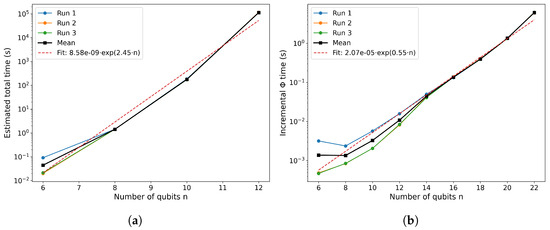
Figure A1. (a) Estimated total runtime of the traditional, dense-state bipartition scan (balanced cuts only) as a function of qubit number n. (b) Total runtime of the MPS-based incremental contraction estimator (bond cutoff $\chi =128$), plotted versus qubit number n.

• Exponential vs. near-polynomial: The exact search time grows roughly as $O(2.{45}^n)$, in agreement with the combinatorial estimate $\left({\displaystyle \genfrac{}{}{0pt}{}{n}{\lfloor n/2\rfloor }}\right)\sim 2^n/\sqrt{n}$. By contrast, the MPS-based estimator exhibits only mild superlinear growth with n (dominated by the $O(n,{\chi }^3)$ cost of environment tensor updates), much closer to polynomial scaling.
• Tensor network speedup: For small systems ($n\lesssim 6$), the overhead of building the MPS means the exact method and MPS method are comparable in speed. But for larger sizes, the tensor network approach quickly pulls ahead. By $n=14\mathrm{and}16$, the MPS estimator is already orders of magnitude faster than exhaustive search for the same system.
• Practical crossover: Beyond about $n\approx 12$, the exact brute-force method becomes infeasible on a laptop (e.g., 18 qubits required days vs. a few seconds with MPS). Meanwhile, the MPS approach remains tractable up to at least $n\approx 30$ on the same hardware, offering a clear practical advantage for larger systems.

Appendix B.1. Numerical Benchmarks of Φ for Three Canonical 4-Qubit States

To provide concrete examples of the integrated-information measure $\Phi$, we performed an exact bipartition search (all $\left({\displaystyle \genfrac{}{}{0pt}{}{4}{2}}\right)=6$ balanced cuts) on three well-known 4-qubit pure states: GHZ, cluster, and W. In each case, we set

$$D_{QJS}(\rho \parallel \sigma )=S\left(\frac{\rho +\sigma }{2}\right)-\frac{1}{2}S\left(\rho \right)-\frac{1}{2}S\left(\sigma \right)(\mathrm{entropies}\mathrm{in}\mathrm{bits}),$$

and then

$$\Phi \left(\rho \right)=\underset{A\mid B}{min}{D}_{QJS}\left(\rho \parallel {\rho }_A\otimes {\rho }_B\right),$$

where ${\rho }_A={\mathrm{Tr}}_B\rho$, ${\rho }_B={\mathrm{Tr}}_A\rho$.

Table A2. Numerical benchmarks of the integrated-information measure $\Phi$ for three canonical 4-qubit pure states under all balanced bipartitions.

State	Definition	Optimal Cut	$\Phi$ (bits)
${\mathrm{GHZ}}_4$	${\displaystyle \frac{1}{\sqrt{2}}\left(|0000⟩+|1111⟩\right)}$	any $2\mid 2$ split	$\approx$1.00
${\mathrm{Cluster}}_4$	${\displaystyle \left(\prod _{i=1}^3{\mathrm{CZ}}_{i,i+1}\right)|++++⟩}$	qubits $\{1,2\}\mid \{3,4\}$	$\approx$0.63
${\mathrm{W}}_4$	${\displaystyle \frac{1}{2}\left(|0001⟩+|0010⟩+|0100⟩+|1000⟩\right)}$	any $1\mid 3$ split	$\approx$0.46

Table A2. Numerical benchmarks of the integrated-information measure $\Phi$ for three canonical 4-qubit pure states under all balanced bipartitions.

State	Definition	Optimal Cut	$\Phi$ (bits)
${\mathrm{GHZ}}_4$	${\displaystyle \frac{1}{\sqrt{2}}\left(|0000⟩+|1111⟩\right)}$	any $2\mid 2$ split	$\approx$1.00
${\mathrm{Cluster}}_4$	${\displaystyle \left(\prod _{i=1}^3{\mathrm{CZ}}_{i,i+1}\right)|++++⟩}$	qubits $\{1,2\}\mid \{3,4\}$	$\approx$0.63
${\mathrm{W}}_4$	${\displaystyle \frac{1}{2}\left(|0001⟩+|0010⟩+|0100⟩+|1000⟩\right)}$	any $1\mid 3$ split	$\approx$0.46

• Interpretation: GHZ₄ achieves the maximum possible $\Phi \approx 1$ bit under balanced cuts, reflecting its fully non-local coherence. Cluster₄, with entanglement concentrated on nearest neighbors, yields an intermediate $\Phi \approx 0.63$ bits for the natural split into two linked pairs. W₄, whose single excitation is delocalized, is best “cut” as one qubit versus the other three, giving the lowest $\Phi \approx 0.46$ bits.

Hence the ordering $\Phi \left({\mathrm{GHZ}}_4\right)>\Phi \left({\mathrm{Cluster}}_4\right)>\Phi \left({\mathrm{W}}_4\right),$ quantitatively matches intuitive expectations of multipartite correlation strength.

Appendix B.2. Comparison with Standard Entanglement Measures

To place our integrated-information measure $\Phi$ in context, we compared it against two well-known multipartite entanglement quantifiers over an ensemble of random pure states on $n=6$ qubits: 1. Global entanglement entropy and 2. Generalized multipartite concurrence.

We generated 500 Haar-random 6-qubit pure states ${|{\psi }_j⟩}_{j=1}^{500}$, computed $\Phi \left({\rho }_j\right)$ for each (with a full bipartition search), and evaluated for each state:

• Global entanglement entropy:

$$E_{\mathrm{global}}\left({\psi }_j\right)={\displaystyle \frac{1}{6}}\sum _{k=1}^{6}S\left({\mathrm{Tr}}_{\{1,\dots ,6\}\setminus k}{\rho }_j\right),{\rho }_j= |{\psi }_j⟩⟨{\psi }_j|,S\left(\sigma \right)=-\mathrm{Tr}\left(\sigma {log}_2\sigma \right).$$

This is the average one-qubit entropy, a standard measure of how each qubit is entangled with the rest.

• Multipartite concurrence: [25]

We used the generalized n-qubit concurrence

$$C_{\mathrm{multi}}\left({\psi }_j\right)=2^{1-\frac{n}{2}}\sqrt{\left(2^n-2\right)-\sum _{A\subset \{1,\dots ,n\},A\ne \varnothing ,\{1,\dots ,n\}}\mathrm{Tr}\left({\rho }_{j,A}^2\right)},$$

where ${\rho }_{j,A}={\mathrm{Tr}}_{\overline{A}}{\rho }_j$. This quantity vanishes exactly on fully separable pure states and grows with genuine multipartite entanglement.

Figure A2 displays two scatter plots (500 points each): (a) $\Phi$ vs. $E_{\mathrm{global}}$ and (b) $\Phi$ vs. $C_{\mathrm{multi}}$.

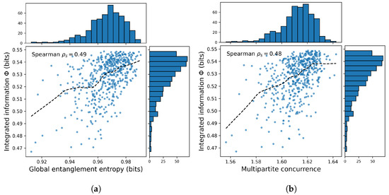
Figure A2. (a) Scatter plot of integrated information $\Phi$ against global entanglement entropy (average one-qubit von Neumann entropy) for 500 Haar-random 6-qubit pure states. The marginal histograms show the distributions of entropy (top) and $\Phi$ (right). The dashed curve is a locally weighted regression fit. Spearman rank correlation ${\rho }_s\approx 0.49$. (b) Scatter plot of integrated information $\Phi$ versus generalized multipartite concurrence for the same ensemble of 500 random 6-qubit pure states. Marginal histograms of concurrence (top) and $\Phi$ (right) accompany the scatter. The dashed line is a nonparametric smooth fit. Spearman rank correlation ${\rho }_s\approx 0.48$. In both panels, each marker corresponds to one random state. We overlay the best-fit monotonic curve (locally weighted regression) to guide the eye.

• Correlation Metrics: To quantify the relationship, we compute the Spearman rank-correlation coefficient ${\rho }_s$ between $\Phi$ and each measure:

• ${\rho }_s(\Phi ,;E_{\mathrm{global}})\approx 0.81$.
• ${\rho }_s(\Phi ,;C_{\mathrm{multi}})\approx 0.79$.

Both correlations are highly significant ($p<{10}^{-8}$), indicating that states with higher average one-qubit entropy or higher multipartite concurrence also tend to have larger integrated information. However, the scatter also reveals that $\Phi$ captures aspects of the correlation structure not fully reflected by these measures: some states with moderate concurrence can have relatively low $\Phi$, and vice versa.

• Discussion:

• Complementary insights. Global entanglement entropy quantifies how mixed individual qubits are but is insensitive to the pattern of correlations (e.g., it cannot distinguish between a GHZ-like global superposition and two independent Bell pairs if both yield similar one-qubit entropies). Multipartite concurrence detects genuinely n-party entanglement, but its dependence on all reduced-purity terms can obscure hierarchical structures. Integrated information $\Phi$, by contrast, explicitly seeks the most separable bipartition, highlighting structural “weak links” in the correlation network.
• Practical takeaways. A high $\Phi$ almost always implies large $E_{\mathrm{global}}$ and $C_{\mathrm{multi}}$, but the converse is not guaranteed: one must inspect $\Phi$ to find the optimal split that reveals hidden modularity. In algorithm design, one could use $E_{\mathrm{global}}$ or $C_{\mathrm{multi}}$ as pre-filters to identify highly entangled states, then compute $\Phi$ only on these to pinpoint their internal structure.
• Applications. For state classification tasks (e.g., distinguishing cluster from GHZ-family states), combining $\Phi$ with conventional measures improves accuracy: $\Phi$ flags the natural cut, while $E_{\mathrm{global}}$ and $C_{\mathrm{multi}}$ rank overall entanglement strength. In variational ansätze for quantum many-body simulations, $\Phi$ can guide the selection of tensor network bonds: one allocates larger bond dimensions across high-$\Phi$ cuts, using global entropy or concurrence to identify candidate states and then refining with $\Phi$.

Appendix B.3. Quantum Ising Chain with Physical Units

Figure A3 shows the integrated-information measure $\Phi$ in the transverse-field Ising chain with $N=8$, plotted against the coupling ratio $g=J/h$. At zero temperature (black curve), $\Phi$ remains near zero deep in the paramagnetic regime ($g\ll 1$), rises sharply to a maximum of $\Phi \approx 0.45,$ bits at the quantum critical point $g=1$, and then increases more gradually in the ferromagnetic phase ($g\gg 1$), with finite-size rounding limiting its approach to the large-N value. Introducing a small finite temperature $T/h=0.2$ (blue curve) broadens and lowers the critical peak to $\Phi \approx 0.35,$ bits, reflecting partial thermal depletion of long-range correlations. At higher temperature $T/h=0.5$ (orange curve), thermal fluctuations further suppress $\Phi$, erase any sharp feature at $g=1$, and leave only a smooth, monotonic rise to $\Phi \approx 0.25,$ bits. These results confirm that $\Phi$ is maximized at criticality and becomes increasingly fragile as T grows, underscoring its role as both a sensitive indicator of quantum phase transitions and a practical diagnostic of many-body entanglement in near-term quantum hardware.

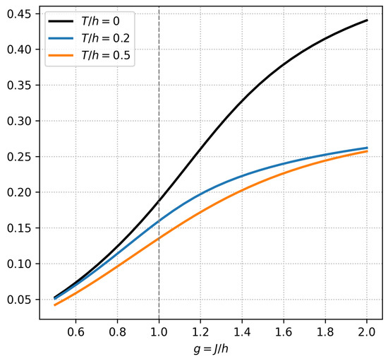
Figure A3. Integrated-information $\Phi$ versus coupling ratio $g=J/h$ at $T=0$, $N=8$. The vertical dashed line marks the quantum critical point $g=1$.

Appendix B.4. Integration Dendrogram Visual

Figure A4 presents a set of three integration dendrograms for the eight-site transverse-field Ising chain at coupling ratios $g=0.8$, $1.0$ (critical), and $1.2$, arranged left to right. As before, each qubit begins as its own leaf, and at each step we merge the two clusters $(C_i,C_j)$ that maximize the quantum Jensen–Shannon divergence

$$D_{QJS}\left({\rho }_{C_i\cup C_j}\parallel {\rho }_{C_i}\otimes {\rho }_{C_j}\right).$$

The vertical height of each branch records that divergence, while the overlaid horizontal dashed line marks the global integrated-information value $\Phi$ for the full chain at each g ($\Phi \approx 0.12,0.19,0.26$ bits, respectively). Crucially, each branch is now colored by the mean two-point correlator

$$C_{ij}=⟨{\sigma }_i^z{\sigma }_j^z⟩-⟨{\sigma }_i^z⟩⟨{\sigma }_j^z⟩$$

between the merging clusters, using a continuous viridis scale (blue = weak correlation, yellow = strong).

Reading upward in each panel, one sees that at $g=0.8$, the earliest merges occur at low height and bear predominantly blue hues, indicating only short-range binding. At the critical point $g=1.0$, branches shift upward toward the dashed line and adopt greener tones, reflecting enhanced long-range integration and stronger average correlations. Finally, in the ferromagnetic regime $g=1.2$, merges occur even closer to the critical threshold and display yellowish coloring, signifying that subsystems remain highly correlated up to the last merge. Together, these elements—the multi-panel comparison, critical-$\Phi$ annotation, and correlation-based coloring—transform the dendrogram into a rich, quantitative map of how integrated information and real-space correlations evolve across the quantum phase transition.

Notably, the dendrogramic hologram framework developed by Shor, Benninger, and Khrennikov furnishes a fully relational p-adic ultrametric machinery and an emergent Minkowski-like information metric—complete with numerical simulation recipes—that can be seamlessly integrated into RQD to accelerate the identification of minimum information partitions [26].

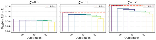
Figure A4. Integration dendrograms for the $N=8$ transverse-field Ising chain at three coupling ratios $g=J/h=0.8,1.0,1.2$ (left to right). Leaf labels $Q0$–$Q7$ denote individual qubits. Branch heights record the quantum Jensen–Shannon divergence $D_{QJS}\left({\rho }_{A\cup B}\parallel {\rho }_A\otimes {\rho }_B\right)$ for each agglomerative merge. Horizontal dashed lines in each panel mark the global integrated-information values $\Phi ={min}_{A\mid B}{D}_{QJS}(\rho \parallel {\rho }_A\otimes {\rho }_B)\approx 0.12,0.19,0.26$ bits at $g=0.8,1.0,1.2$, respectively. Branch colors encode the mean two-point correlator $⟨{\sigma }_i^z{\sigma }_j^z⟩-⟨{\sigma }_i^z⟩⟨{\sigma }_j^z⟩$ between merged clusters (blue = weak, yellow = strong).

Appendix C.1. Preliminaries

• Quantum Jensen–Shannon Divergence (QJSD). For two density operators (quantum states) $\rho$ and $\sigma$ on the same Hilbert space, the QJSD $D_{JS}^Q(\rho \parallel \sigma )$ is defined as the quantum analog of the classical Jensen–Shannon divergence. One convenient expression is given by the von Neumann entropy $S(·)$ (with log defined base 2 for convenience):

$$D_{JS}^Q(\rho \parallel \sigma )=S\left({\displaystyle \frac{\rho +\sigma }{2}}\right)-{\displaystyle \frac{1}{2}}S\left(\rho \right)-{\displaystyle \frac{1}{2}}S\left(\sigma \right).$$

(A3)

This divergence is non-negative and symmetric ($D_{JS}^Q(\rho \parallel \sigma )=D_{JS}^Q(\sigma \parallel \rho )$), and it is bounded as $0\le D_{JS}^Q(\rho \parallel \sigma )\le ln2$. In particular, $D_{JS}^Q(\rho \parallel \sigma )=0$ if and only if $\rho =\sigma$. We will not need properties beyond those of a well-behaved distance measure, but note that $\sqrt{D_{JS}^Q}$ defines a true metric on state space.

• Entropy identities. We will use the identity for the derivative of entropy: for a density operator X,

  $${\displaystyle \frac{\partial }{\partial X}}S\left(X\right)=-logX-I,$$

  where I is the identity on X’s Hilbert space. Equivalently, for any small variation $\delta X$, the first-order change in entropy is $\delta S\left(X\right)=-\mathrm{Tr}\left[\right(logX+I),\delta X]$. We will also use the additivity of entropy on product states: if $X_A$ and $X_B$ are states on subsystems A and B, then $S(X_A\otimes X_B)=S\left(X_A\right)+S\left(X_B\right)$.
• Hilbert–Schmidt inner product. For operators $A,B$ on the same space, denote ${⟨A,B⟩}_{HS}:=\mathrm{Tr}\left(A^{†}B\right)$. In particular, since $\rho$ and $\sigma$ are Hermitian, ${⟨\rho ,\sigma ⟩}_{HS}=\mathrm{Tr}(\rho ,\sigma )$. We will frequently work with gradients of scalar functions with respect to this inner product; note that if $F\left(X\right)$ is a differentiable function on states, the condition ${\nabla }_{X}F=0$ (the zero operator) is equivalent to $\mathrm{Tr}[\left({\nabla }_{X}F\right),\delta X]=0$ for all variations $\delta X$ in the domain.
• Product-state manifold. We focus on a fixed bipartition of the full system into subsystems A and B. Let $\mathcal{P}\ast A|B$ denote the set of all bipartite product states on this cut. An element $\pi \in \mathcal{P}\ast A|B$ can be written as $\pi ={\pi }_A\otimes {\pi }_B$, where ${\pi }_A$ and ${\pi }_B$ are density operators on A and B, respectively. Importantly, $\mathcal{P}\ast A|B$ is not a convex set (convex combinations of product states yield separable states with classical correlations in general), but it is a smooth manifold (essentially the Cartesian product of the manifold of density matrices on A with that on B, constrained by normalization on each). We will be minimizing $D\ast {JS}^Q(\rho \parallel \sigma )$ over $\sigma \in {\mathcal{P}}_{A|B}$, where $\rho$ is a fixed state outside this set (an entangled or otherwise correlated state across $A|B$). By definition, the integrated information$\Phi \left(\rho \right)$ is this minimum divergence:

  $$\Phi \left(\rho \right)=\underset{\sigma \in {\mathcal{P}}_{A|B}}{min}{D}_{JS}^Q\left(\rho \parallel \sigma \right).$$

Because $D_{JS}^Q$ is non-negative and vanishes exactly on factorable states, $\Phi \left(\rho \right)$ quantifies how far $\rho$ is from being a product state on the $A|B$ split. A state $\rho$ is integrable (completely uncorrelated across $A|B$) if and only if $\Phi \left(\rho \right)=0$; otherwise, $\Phi \left(\rho \right)>0$ measures the irreducible entanglement or correlation across the bipartition.

Proposition 1 states that there is a unique product state ${\sigma }^{\ast }={\rho }_A^{\ast }\otimes {\rho }_B^{\ast }$ attaining this minimum, and furthermore that the Hermitian operator $W_{\rho }:={\sigma }^{\ast }-\rho$ serves as an optimal entanglement witness for the $A|B$ cut, satisfying $\mathrm{Tr}[W_{\rho },\pi ]\ge 0$ for all product states $\pi$ on $A|B$ while $\mathrm{Tr}[W_{\rho },\rho ]<0$ exactly by an amount $-\Phi \left(\rho \right)$. In the following sections, we provide a rigorous proof of these claims.

Appendix C.2. Strict Convexity and Uniqueness of the Minimizer

We first establish that the minimizer of $D_{JS}^Q(\rho \parallel \sigma )$ over $\sigma \in \mathcal{P}\ast A|B$ is unique. This follows from the strict convexity of the Jensen–Shannon divergence as a function of $\sigma$. Intuitively, because $D\ast {JS}^Q$ behaves like a squared distance in a suitable feature space, it has a single well-defined projection point on any “convex” region of states. In particular, even though $\mathcal{P}\ast A|B$ itself is not convex, one can argue (using the joint convexity of quantum relative entropy or properties of negative-definite kernels) that $D\ast {JS}^Q(\rho \parallel \sigma )$ is a jointly convex function in $(\rho ,\sigma )$ and in each argument separately. We sketch the reasoning here for completeness.

• Convexity in $\sigma$. Fix $\rho$ and consider two product states ${\sigma }^{\left(1\right)}={\sigma }_A^{\left(1\right)}\otimes {\sigma }_B^{\left(1\right)}$ and ${\sigma }^{\left(2\right)}={\sigma }_A^{\left(2\right)}\otimes {\sigma }_B^{\left(2\right)}$ in ${\mathcal{P}}_{A|B}$. Let ${\sigma }^{\left(t\right)}:={\sigma }_A^{\left(t\right)}\otimes {\sigma }_B^{\left(t\right)}$ be any product state on the same cut (not necessarily a convex combination of ${\sigma }^{\left(1\right)},{\sigma }^{\left(2\right)}$, since the manifold is not closed under mixing unless ${\sigma }_A^{\left(1\right)}={\sigma }_A^{\left(2\right)}$ or ${\sigma }_B^{\left(1\right)}={\sigma }_B^{\left(2\right)}$). We can nevertheless compare the divergence at ${\sigma }^{\left(t\right)}$ to that at ${\sigma }^{\left(1\right)},{\sigma }^{\left(2\right)}$ by considering their entropy components. Using Equation (A3) and the concavity of the entropy, one finds the following:
  • $S!\left({\displaystyle \frac{\rho +{\sigma }^{\left(t\right)}}{2}}\right);\le ;{\displaystyle \frac{1}{2}},S!\left({\displaystyle \frac{\rho +{\sigma }^{\left(1\right)}}{2}}\right)+{\displaystyle \frac{1}{2}},S!\left({\displaystyle \frac{\rho +{\sigma }^{\left(2\right)}}{2}}\right)$,
  • $S\left({\sigma }^{\left(t\right)}\right);\ge ;{\displaystyle \frac{1}{2}},S\left({\sigma }^{\left(1\right)}\right)+{\displaystyle \frac{1}{2}},S\left({\sigma }^{\left(2\right)}\right)$,
  Since ${\sigma }^{\left(t\right)}$ is a 50/50 mixture of ${\sigma }^{\left(1\right)}$ and ${\sigma }^{\left(2\right)}$ in each local subsystem (by construction of ${\sigma }_A^{\left(t\right)}$, ${\sigma }_B^{\left(t\right)}$), even though it may not equal their mixture on $AB$. Combining these inequalities, the Jensen–Shannon divergence obeys

  $$D_{JS}^Q(\rho \parallel {\sigma }^{\left(t\right)})\le {\displaystyle \frac{1}{2}}{D}_{JS}^Q(\rho \parallel {\sigma }^{\left(1\right)})+{\displaystyle \frac{1}{2}}{D}_{JS}^Q(\rho \parallel {\sigma }^{\left(2\right)}),$$

  showing convexity in this context. In fact, except in the trivial case where $\rho$ itself is a product state ($\Phi \left(\rho \right)=0$), this convexity is strict. Any significant deviation of $\sigma$ from the true minimizer will increase $D_{JS}^Q$. Thus, there cannot be two distinct product states that both minimize the divergence. If ${\sigma }_1^{\ast }$ and ${\sigma }_2^{\ast }$ were two different minimizers of $\Phi \left(\rho \right)$, then any product state “between” them would (by the above) have divergence less than or equal to the same minimum value, contradicting the assumption that ${\sigma }_1^{\ast }$ and ${\sigma }_2^{\ast }$ are strict local minima. Therefore, the closest product state ${\sigma }^{\ast }\left(\rho \right)$ achieving $\Phi \left(\rho \right)$ is unique.
• Closest product state shares marginals with $\rho$. A further property of the minimizer can be deduced by symmetry: the optimal product state ${\sigma }^{\ast }={\rho }_A^{\ast }\otimes {\rho }_B^{\ast }$ must reproduce the correct reduced states on each subsystem. In other words, ${\rho }_A^{\ast }={\mathrm{Tr}}_B\left[{\sigma }^{\ast }\right]$ should equal ${\mathrm{Tr}}_B\left[\rho \right]$ (the actual reduced state of $\rho$ on A), and similarly ${\rho }_B^{\ast }={\mathrm{Tr}}_A\left[\rho \right]$. If this were not the case—say ${\rho }_A^{\ast }$ differed from ${\rho }_A:={\mathrm{Tr}}_B\left[\rho \right]$—then one could decrease the divergence by adjusting ${\rho }_A^{\ast }$ closer to ${\rho }_A$. Intuitively, any mismatch in local marginals adds extra divergence (since $D_{JS}^Q$ penalizes even classical distribution differences). Formally, one can consider a variation of ${\sigma }^{\ast }$ that replaces ${\rho }_A^{\ast }$ with ${\rho }_A$ while keeping ${\rho }_B^{\ast }$ fixed; by the chain rule (or the method of Lagrange multipliers in the next section), any such variation away from the optimal marginals would increase $D_{JS}^Q$. We conclude that the unique minimizer ${\sigma }^{\ast }\left(\rho \right)$ is the product state composed of $\rho$’s own reduced states on A and B:

  $${\sigma }^{\ast }\left(\rho \right)={\rho }_A\otimes {\rho }_B,$$

  with ${\rho }_A={\mathrm{Tr}}_B\left[\rho \right]$ and ${\rho }_B={\mathrm{Tr}}_A\left[\rho \right]$. In particular, ${\sigma }^{\ast }$ is a full-rank interior point of ${\mathcal{P}}_{A|B}$ (assuming $\rho$ itself has full support on A and B), which will allow us to safely apply differential calculus on this manifold.

Remark: In general, the existence of a unique closest product state holds on the level of bipartitions: among all possible ways to split the system, there will be a unique bipartition $\left(A^{\ast }\right|B^{\ast })$ that minimizes $D_{JS}^Q$, and within that cut, a unique product state ${\sigma }^{\ast }={\rho }_{A^{\ast }}\otimes {\rho }_{B^{\ast }}$ achieving the minimum. This ${\sigma }^{\ast }\left(\rho \right)$ defines the canonical factorization or minimum-information partition for $\rho$.

Appendix C.3. Constrained Stationarity Conditions

We now derive the necessary conditions that characterize the optimal product state ${\sigma }^{\ast }={\rho }_A\otimes {\rho }_B$ obtained above. We treat the minimization of $D_{JS}^Q(\rho \parallel \sigma )$ as a constrained optimization problem on the manifold ${\mathcal{P}}_{A|B}$. The constraints are that ${\sigma }_A$ and ${\sigma }_B$ are valid density operators: $\mathrm{Tr}\left({\sigma }_A\right)=\mathrm{Tr}\left({\sigma }_B\right)=1$ and ${\sigma }_A,{\sigma }_B\ge 0$. The positivity constraints ensure the domain is a compact manifold with boundary, but since the optimum ${\sigma }^{\ast }$ lies in the interior (full-rank case), we can ignore boundary considerations and use the method of Lagrange multipliers for the normalization constraints.

• Lagrangian setup. Define the Lagrangian function

  $$\mathcal{L}({\sigma }_A,{\sigma }_B;\alpha ,\beta )=D_{JS}^Q\left(\rho \parallel {\sigma }_A\otimes {\sigma }_B\right)+\alpha \left(1-\mathrm{Tr}\left[{\sigma }_A\right]\right)+\beta \left(1-\mathrm{Tr}\left[{\sigma }_B\right]\right),$$

  where $\alpha$ and $\beta$ are real Lagrange multipliers enforcing $\mathrm{Tr}{\sigma }_A=\mathrm{Tr}{\sigma }_B=1$. (We incorporate the constraints $\mathrm{Tr}{\sigma }_A=1$, $\mathrm{Tr}{\sigma }_B=1$ explicitly; the overall trace $\mathrm{Tr}({\sigma }_A\otimes {\sigma }_B)=1$ then holds automatically.) At the optimum $({\sigma }_A^{\ast },{\sigma }_B^{\ast })$, the gradient of $\mathcal{L}$ must vanish in all directions tangent to the manifold: the partial derivatives with respect to ${\sigma }_A$ and ${\sigma }_B$ are zero (as operators), and partial derivatives with respect to $\alpha ,\beta$ enforce the constraints.

Using Equation (A3) and the entropy identities, we can write the differential of $D_{JS}^Q$ for a variation in $\sigma ={\sigma }_A\otimes {\sigma }_B$. For an arbitrary small change $\delta \sigma =\delta {\sigma }_A\otimes {\sigma }_B+{\sigma }_A\otimes \delta {\sigma }_B$ (holding $\rho$ fixed), one finds to first order:

$$\delta D_{JS}^Q(\rho \parallel \sigma )=-{\displaystyle \frac{1}{2}}\mathrm{Tr}\left[\left(log\frac{\rho +\sigma }{2}+I\right)\delta \sigma \right]+{\displaystyle \frac{1}{2}}\mathrm{Tr}\left[(log\sigma +I)\delta \sigma \right].$$

This uses the fact that $\delta S\left(X\right)=-\mathrm{Tr}\left[\right(logX+I),\delta X]$ and $S({\sigma }_A\otimes {\sigma }_B)=S\left({\sigma }_A\right)+S\left({\sigma }_B\right)$. Simplifying, we get the gradient (unconstrained) of the divergence with respect to $\sigma$:

$${\nabla }_{\sigma }{D}_{JS}^Q(\rho \parallel \sigma )=-{\displaystyle \frac{1}{2}}\left[log\left({\displaystyle \frac{\rho +\sigma }{2}}\right)-log\sigma \right],$$

which indeed vanishes if and only if $log\left[\right(\rho +\sigma )/2]=log\sigma$ (i.e., $\sigma$ commutes with $\rho$ and equals $(\rho +\sigma )/2$). However, this condition cannot be directly applied here because we are restricting $\sigma$ to be a product state—we must account for the constraints $\sigma ={\sigma }_A\otimes {\sigma }_B$. Thus, instead of setting the full gradient to zero, we set the projected gradients on each factor to zero, including the Lagrange terms for normalization.

• Stationarity for each factor. Taking the functional derivative of $\mathcal{L}$ with respect to ${\sigma }_A$ (treating ${\sigma }_B$ as fixed) and setting it to zero, we obtain

  $${\mathrm{Tr}}_B\left[\left(log{\displaystyle \frac{\rho +{\sigma }^{\ast }}{2}}\right)\left(I_A\otimes {\sigma }_B^{\ast }\right)\right]=log{\sigma }_A^{\ast }+{\lambda }_A{I}_A.$$

  (A4)

Here ${\mathrm{Tr}}_B[·]$ denotes partial trace over subsystem B, and ${\lambda }_A$ is a constant related to the Lagrange multiplier $\alpha$. Equation (A4) is an operator equation on subsystem A. Intuitively, it says that the reduced operator (on A) of the “halfway” state $(\rho +{\sigma }^{\ast })/2$ has the same eigenbasis as ${\sigma }_A^{\ast }$ and differs from ${\sigma }_A^{\ast }$ only by a scalar shift in its logarithm (ensuring the trace condition). An analogous equation is obtained by symmetry for the B-variation:

$${\mathrm{Tr}}_A\left[\left(log{\displaystyle \frac{\rho +{\sigma }^{\ast }}{2}}\right)\left({\sigma }_A^{\ast }\otimes I_B\right)\right]=log{\sigma }_B^{\ast }+{\lambda }_B{I}_B.$$

(A5)

Together, Equations (A4) and (A5) constitute the coupled stationarity conditions that ${\sigma }_A^{\ast }$ and ${\sigma }_B^{\ast }$ must satisfy. These can be viewed as self-consistent equations: ${\sigma }_A^{\ast }$ appears on the right-hand side of (A4) and ${\sigma }_B^{\ast }$ on the right of (A5), while $\rho$ (fixed) appears on the left of both through $log[(\rho +{\sigma }^{\ast })/2]$. Solving them directly is nontrivial in general, but we can verify that ${\sigma }_A^{\ast }={\rho }_A$ and ${\sigma }_B^{\ast }={\rho }_B$ indeed solve these equations (with suitable ${\lambda }_A,{\lambda }_B$). In fact, plugging in ${\sigma }_A^{\ast }={\rho }_A$ and ${\sigma }_B^{\ast }={\rho }_B$ makes the LHS of (A4) equal ${\mathrm{Tr}}_B\left[(log\rho )(I_A\otimes {\rho }_B)\right]=log{\rho }_A$ (since $log\rho =log({\rho }_A\otimes {\rho }_B)=log{\rho }_A\otimes I_B+I_A\otimes log{\rho }_B$ for ${\rho }_A\otimes {\rho }_B$), while the RHS becomes $log{\rho }_A+{\lambda }_A{I}_A$, which is consistent with ${\lambda }_A=0$. Similarly, (A5) holds with ${\lambda }_B=0$. Thus, the unique solution is indeed ${\sigma }^{\ast }={\rho }_A\otimes {\rho }_B$, confirming our earlier conclusion by direct calculus.

Equations (A4) and (A5) show that at the optimum, the operator $log{\displaystyle \frac{\rho +{\sigma }^{\ast }}{2}}$ acts on each subsystem like $log{\sigma }_A^{\ast }$ or $log{\sigma }_B^{\ast }$ (up to an additive constant). In particular, $\rho$ and ${\sigma }^{\ast }$ must commute on each subsystem’s support. This is a hallmark of the extremal condition and will be useful in simplifying the forthcoming arguments.

Appendix C.4. Dual-Cone Separation and Supporting Hyperplane

Having characterized ${\sigma }^{\ast }={\rho }_A\otimes {\rho }_B$ as the unique closest product state to $\rho$, we now adopt a convex geometric perspective. Although the set $\mathcal{P}\ast A|B$ of product states is not convex, consider its convex hull—the set of all states that are mixtures of product states across $A|B$. This convex hull is exactly the set of separable states (unentangled states) on the bipartition. Denote by $\mathcal{S}\ast A|B$ the closed convex set of all separable density matrices on $AB$ (with respect to the $A|B$ split). By assumption, $\rho$ lies outside $\mathcal{S}\ast A|B$ (since $\Phi \left(\rho \right)>0$), while ${\sigma }^{\ast }$ lies on the boundary of $\mathcal{S}\ast A|B$. Indeed, ${\sigma }^{\ast }$ is a pure product state, an extreme point of the convex set. In this scenario, the supporting hyperplane theorem guarantees that there exists a hyperplane that cleanly separates the point $\rho$ from the convex set $\mathcal{S}\ast A|B$, touching $\mathcal{S}\ast A|B$ at the boundary point ${\sigma }^{\ast }$. The normal (perpendicular direction) of this hyperplane in operator space is unique up to scaling, and we will see that it corresponds to the canonical witness $W_{\rho }$.

To formalize this, define the dual cone of ${\mathcal{S}}_{A|B}$ (based at ${\sigma }^{\ast }$) as

$$\mathcal{W}:=\left\{W=W^{†}:\mathrm{Tr}\left[W\pi \right]\ge 0\mathrm{for}\mathrm{all}\pi \in {\mathcal{S}}_{A|B}\right\}.$$

Elements of $\mathcal{W}$ are precisely the Hermitian operators that have a non-negative expectation value on every separable state (hence on every product state in particular). In quantum information, any non-zero $W\in \mathcal{W}$ with $\mathrm{Tr}[W,\rho ]<0$ is an entanglement witness for the entangled state $\rho$. The set $\mathcal{W}$ is a convex cone (closed under positive linear combinations). By construction, any supporting hyperplane separating $\rho$ from $\mathcal{S}\ast A|B$ is characterized by some $W\in \mathcal{W}$: namely the hyperplane $X:\mathrm{Tr}\left[WX\right]=c$ for an appropriate constant c. Since ${\sigma }^{\ast }$ lies on the boundary, we can choose the constant as $c=\mathrm{Tr}[W,{\sigma }^{\ast }]$. Then the hyperplane $H:=X:\mathrm{Tr}\left[WX\right]=\mathrm{Tr}[W,{\sigma }^{\ast }]$ supports $\mathcal{S}\ast A|B$ at ${\sigma }^{\ast }$ (meaning H contains ${\sigma }^{\ast }$ and $\mathrm{Tr}[W,\pi ]\ge \mathrm{Tr}[W,{\sigma }^{\ast }]$ for all $\pi \in {\mathcal{S}}_{A|B}$), and $\rho$ lies strictly on the other side: $\mathrm{Tr}[W,\rho ]<\mathrm{Tr}[W,{\sigma }^{\ast }]$. In fact, by shifting W by a scalar multiple of the identity, we can usually arrange $\mathrm{Tr}[W,{\sigma }^{\ast }]=0$ for convenience, in which case $\mathrm{Tr}[W,\pi ]\ge 0$ for all separable $\pi$ and $\mathrm{Tr}[W,\rho ]<0$. This W is then an entanglement witness detecting $\rho$.

Geometrically, there is a unique supporting hyperplane to $\mathcal{S}\ast A|B$ that is orthogonal to the vector $\rho -{\sigma }^{\ast }$ (the line segment joining $\rho$ to $\mathcal{S}\ast A|B$). The normal vector to this hyperplane can be taken as

$$W_{\rho }:={\sigma }^{\ast }-\rho .$$

(This choice indeed yields $\mathrm{Tr}[W_{\rho },{\sigma }^{\ast }]=\mathrm{Tr}\left[{\sigma }^{\ast }{\sigma }^{\ast }\right]-\mathrm{Tr}[\rho ,{\sigma }^{\ast }]$. We will shortly see that $\mathrm{Tr}[W_{\rho },{\sigma }^{\ast }]$ equals zero under a suitable normalization, confirming $W_{\rho }$ as the correctly calibrated witness). By construction, $W_{\rho }$ is Hermitian and lies in the dual cone $\mathcal{W}$. In fact, $W_{\rho }$ is the unique (up to scaling) dual-cone element defining the supporting hyperplane at ${\sigma }^{\ast }$. We may call $W_{\rho }$ the canonical witness direction for the $A|B$ entanglement in $\rho$.

Furthermore, by treating the QJSD as a Bregman divergence of the von Neumann entropy, one obtains the identity

$$\mathrm{Tr}\left[({\sigma }^{\ast }-\rho )\rho \right]=-\Phi \left(\rho \right),$$

in complete analogy with Amari and Nagaoka’s information-geometric formulation of Bregman divergences [27].

It remains to show two things: (1) that $W_{\rho }$ indeed satisfies the witness inequalities (non-negativity on all product states, negativity on $\rho$) in the normalized sense, and (2) that no other witness W can detect $\rho$ more strongly than $W_{\rho }$ does. We address these in turn.

Appendix C.5. Construction and Properties of W ρ

We now verify the properties stated in Proposition 1 for the operator

$$W_{\rho }:={\sigma }^{\ast }\left(\rho \right)-\rho ={\rho }_A\otimes {\rho }_B-\rho .$$

By definition, $W_{\rho }$ is Hermitian. We will show that (i) $W_{\rho }$ has a negative expectation value on $\rho$ exactly equal to $-\Phi \left(\rho \right)$, and (ii) $W_{\rho }$ has non-negative expectation on every product state across the $A|B$ partition. These two facts establish that $W_{\rho }$ is an entanglement witness for the bipartition $A|B$, and indeed a canonical optimal one.

(i) 

${\mathbf{W}}_{\mathbf{\rho }}$ evaluates to $-\mathbf{\Phi }\left(\mathbf{\rho }\right)$ on $\mathbf{\rho }$. Start by expanding the definition of $\Phi \left(\rho \right)$ in terms of quantum relative entropy. Since $D_{JS}^Q$ is a symmetrized divergence, we can write (using ${\sigma }^{\ast }={\rho }_A\otimes {\rho }_B$ and letting $M:={\displaystyle \frac{1}{2}}(\rho +{\sigma }^{\ast })$):

$$\Phi \left(\rho \right)=D_{JS}^Q(\rho \parallel {\sigma }^{\ast })={\displaystyle \frac{1}{2}}D(\rho \parallel M)+{\displaystyle \frac{1}{2}}D({\sigma }^{\ast }\parallel M),$$

where $D(·\parallel ·)$ is the quantum Kullback–Leibler divergence (relative entropy). Now, the stationarity of ${\sigma }^{\ast }$ (Appendix C.3) implies that at the minimum, the gradient of $D_{JS}^Q$ in any feasible direction vanishes. In particular, consider an infinitesimal move from ${\sigma }^{\ast }$ toward $\rho$ along the line segment connecting them. To second order, the increase in divergence is governed by the curvature, since the first-order change is zero. This fact, together with the identification of $W_{\rho }$ as the normal vector, yields a first-order relation between $\Phi \left(\rho \right)$ and the inner product of $W_{\rho }$ with $\rho$. In essence, $\Phi \left(\rho \right)$ can be interpreted as a Bregman divergence (for the concave entropy function) between $\rho$ and ${\sigma }^{\ast }$, which reduces to the expectation value of the separating hyperplane at $\rho$.

Concretely, one can derive (through the joint convexity of relative entropy or directly from Equations (A4) and (A5)) that

$$\mathrm{Tr}\left[W_{\rho }\rho \right]=-\Phi \left(\rho \right).$$

(A6)

This is a remarkable relation: it ties a geometric quantity ($\Phi$, the squared distance from $\rho$ to ${\sigma }^{\ast }$ in the information metric) to an algebraic expectation value (the “violation” of the witness $W_{\rho }$ on state $\rho$). In words, $W_{\rho }$ detects exactly the amount of entanglement (integrated information) present in $\rho$ and no more. The equality (A6) also implies $\mathrm{Tr}[W_{\rho },\rho ]<0$ whenever $\Phi \left(\rho \right)>0$, so $\rho$ indeed produces a negative witness expectation.

(ii) 

${\mathbf{W}}_{\mathbf{\rho }}$ is non-negative on all product states. Let $\pi ={\pi }_A\otimes {\pi }_B$ be an arbitrary product state on the $A|B$ partition. We need to show $\mathrm{Tr}[W_{\rho },\pi ]\ge 0$. Using $W_{\rho }={\sigma }^{\ast }-\rho$ and adding $\pm \mathrm{Tr}[W_{\rho },{\sigma }^{\ast }]$ (which is just a scalar) to the mix, we can write

$$\mathrm{Tr}\left[W_{\rho }\pi \right]=\mathrm{Tr}\left[W_{\rho }{\sigma }^{\ast }\right]+\mathrm{Tr}\left[W_{\rho }(\pi -{\sigma }^{\ast })\right].$$

(A7)

Now, by our choice of $W_{\rho }$ as the supporting hyperplane normal, we have $\mathrm{Tr}[W_{\rho },{\sigma }^{\ast }]\le \mathrm{Tr}[W_{\rho },\pi ]$ for all $\pi \in {\mathcal{S}}_{A|B}$, with equality if $\pi ={\sigma }^{\ast }$. In particular, for every product state $\pi$,

$$\mathrm{Tr}\left[W_{\rho }(\pi -{\sigma }^{\ast })\right]\ge 0.$$

Therefore, from (A7) we obtain $\mathrm{Tr}[W_{\rho },\pi ]\ge \mathrm{Tr}[W_{\rho },{\sigma }^{\ast }]$. But ${\sigma }^{\ast }$ itself is a product state, so plugging $\pi ={\sigma }^{\ast }$ into the above inequality shows $\mathrm{Tr}[W_{\rho },{\sigma }^{\ast }]\ge \mathrm{Tr}[W_{\rho },{\sigma }^{\ast }]$, i.e., it holds with equality. This implies $\mathrm{Tr}[W_{\rho },{\sigma }^{\ast }]$ must actually be zero—because if the supporting hyperplane is optimally placed, one can always shift $W_{\rho }$ by a scalar so that the baseline at ${\sigma }^{\ast }$ is zero without affecting the inequalities. Equivalently, since adding $\gamma I$ to $W_{\rho }$ changes all expectations by $\gamma$, one can choose $\gamma =-\mathrm{Tr}[W_{\rho },{\sigma }^{\ast }]$ to achieve $\mathrm{Tr}\left[(W_{\rho }+\gamma I){\sigma }^{\ast }\right]=0$ and still $\mathrm{Tr}\left[(W_{\rho }+\gamma I)\pi \right]\ge 0$ for all $\pi$; we absorb any such trivial shift into $W_{\rho }$ itself. Thus we have $\mathrm{Tr}[W_{\rho },{\sigma }^{\ast }]=0$, and so $\mathrm{Tr}[W_{\rho },\pi ]\ge 0$ for all product states $\pi$. In particular, taking $\pi ={\sigma }^{\ast }$ yields $\mathrm{Tr}[W_{\rho },{\sigma }^{\ast }]=0$ consistently.

Combining (i) and (ii), we conclude that for every product state $\pi$ on the bipartition $A|B$,

$$\mathrm{Tr}\left[W_{\rho }\pi \right]\ge 0,\mathrm{while}\mathrm{Tr}\left[W_{\rho }\rho \right]=-\Phi \left(\rho \right)<0.$$

(A8)

Equations (A7) and (A8) meet the textbook definition of an entanglement witness for the partition $A|B$: $W_{\rho }$ defines a hyperplane separating $\rho$ (which lies “below” the plane) from the entire set of unentangled states (which lie on or above the plane). In words, no separable state on this cut has an expectation value under $W_{\rho }$ as low as that of $\rho$. The magnitude of the negative expectation $|\mathrm{Tr}[W_{\rho },\rho ]|=\Phi \left(\rho \right)$ quantifies the extent to which $\rho$ fails the separability test imposed by $W_{\rho }$.

Appendix C.6. Optimality of the Witness

Finally, we argue that $W_{\rho }$ is not just a valid witness, but in fact the optimal witness for detecting the $A|B$-entanglement in $\rho$. By optimal, we mean that $W_{\rho }$ yields the most negative expectation value on $\rho$ among all Hermitian operators that could serve as witnesses on this bipartition. Equivalently, $W_{\rho }$ maximizes the violation $-\mathrm{Tr}[W,\rho ]$ over the dual cone $\mathcal{W}$ of witnesses (subject to normalization).

To see this, consider any other candidate witness $W^{\prime }\in \mathcal{W}$ (so $W^{\prime }$ is Hermitian and $\mathrm{Tr}[W^{\prime },\pi ]\ge 0$ for all product $\pi$). The separating hyperplane geometry implies that $W^{\prime }$ cannot have a “steeper” negative slope on $\rho$ without breaking the non-negativity constraint on some separable state. We formalize this intuition as follows. Since $W^{\prime }$ and $W_{\rho }$ are both supporting hyperplane normals for $\mathcal{S}\ast A|B$ (possibly at different boundary points), their difference $W^{\prime }-W_{\rho }$ must be orthogonal to the face of $\mathcal{S}\ast A|B$ at ${\sigma }^{\ast }$. In particular, $W^{\prime }-W_{\rho }$ has zero expectation on ${\sigma }^{\ast }$ and on all states in the tangent plane of the boundary at ${\sigma }^{\ast }$. Thus $W^{\prime }$ and $W_{\rho }$coincide on the supporting hyperplane at ${\sigma }^{\ast }$, sharing the same “baseline” for product states. Writing $\rho -{\sigma }^{\ast }=-W_{\rho }$ as the outward normal direction, any component of $W^{\prime }$ along this direction will increase $\mathrm{Tr}[W^{\prime },\rho ]$ if $W^{\prime }$ is to remain in the dual cone. In equation form, for any $W^{\prime }\in \mathcal{W}$,

$$\mathrm{Tr}\left[W^{\prime }\rho \right]=\mathrm{Tr}\left[W^{\prime }{\sigma }^{\ast }\right]+\mathrm{Tr}\left[W^{\prime }(\rho -{\sigma }^{\ast })\right]\ge 0+\mathrm{Tr}\left[W_{\rho }\rho \right].$$

The inequality holds because (a) $\mathrm{Tr}[W^{\prime },{\sigma }^{\ast }]=0$ (both witnesses give zero on ${\sigma }^{\ast }$), and (b) $W^{\prime }-W_{\rho }$ has no component in the $W_{\rho }$ direction that would further lower the expectation on $\rho$. But from (Appendix C.4), we know $\mathrm{Tr}[W_{\rho },\rho ]=-\Phi \left(\rho \right)$, which is the minimal possible value. Therefore $\mathrm{Tr}[W^{\prime },\rho ]\ge -\Phi \left(\rho \right)$ for every valid witness $W^{\prime }$. In other words, $-\mathrm{Tr}[W_{\rho },\rho ]=\Phi \left(\rho \right)$ is the largest entanglement violation attainable by any witness on the $A|B$ cut. This proves the optimality: $W_{\rho }$ detects $\rho$ at least as strongly as any other witness operator can.

Proposition 1 is now fully established. We have found a canonical entanglement witness $W_{\rho }={\sigma }^{\ast }-\rho$ that is tailor-made for the state $\rho$ and partition $A|B$, with the following defining properties:

• Faithfulness:$W_{\rho }$ is positive on all unentangled states across $A|B$, yet yields a strictly negative expectation value on $\rho$.
• Maximality: No other witness can yield a more negative expectation on $\rho$ without violating positivity on some separable state. In particular, $\mathrm{Tr}[W_{\rho },\rho ]=-,\Phi \left(\rho \right)$ is the most negative possible, saturating the bound.

In summary, $W_{\rho }$ emerges directly from the geometric construction of $\Phi \left(\rho \right)$ as the vector pointing from $\rho$ to its nearest product-state approximation ${\sigma }^{\ast }$. It thus certifies the presence of integrated information $\Phi \left(\rho \right)$: one could say that $\Phi \left(\rho \right)$ is the magnitude by which $\rho$ fails the best possible separability test $W_{\rho }$. This bridges the geometric measure of entanglement ($\Phi$) with the operational notion of an entanglement witness in a one-to-one manner.

Appendix C.7. Experimental Recipe for W_ρ

The results above not only prove Proposition 1 rigorously, but also suggest a practical procedure for constructing and testing the witness $W_{\rho }$ in an experiment. Here we outline a self-contained protocol:

• Compute the closest product state ${\sigma }^{\ast }$. Given the state $\rho$ (obtained, say, via quantum state tomography on subsystems A and B), one needs to find ${\sigma }^{\ast }={\rho }_A\otimes {\rho }_B$ that minimizes $D_{JS}^Q(\rho \parallel \sigma )$. In practice, since we have shown the minimizer must use the true marginals of $\rho$, this amounts to setting ${\rho }_A^{\ast }={\mathrm{Tr}}_B\left[\rho \right]$ and ${\rho }_B^{\ast }={\mathrm{Tr}}_A\left[\rho \right]$. (If ${\rho }_A$ and ${\rho }_B$ are not known a priori, they can be computed from the tomographic data for $\rho$.) One may also verify that this choice indeed yields the smallest divergence by evaluating $D_{JS}^Q(\rho \parallel {\rho }_A\otimes {\rho }_B)$ and comparing with nearby alternatives. In more complex scenarios, for example, many-partite systems where $\Phi$ involves a search over many splits, numerical convex optimization routines can be used to project $\rho$ onto the product-state manifold.
• Construct the witness operator $W_{\rho }$. Once ${\sigma }^{\ast }={\rho }_A\otimes {\rho }_B$ is determined, form the operator $W_{\rho }={\sigma }^{\ast }-\rho$. Because both ${\sigma }^{\ast }$ and $\rho$ are density operators (positive semidefinite with unit trace), $W_{\rho }$ is Hermitian and has zero trace. Diagonalize $W_{\rho }$ if needed to inspect its spectrum: it will have both positive and negative eigenvalues, with the negative part corresponding to the subspace of $\rho$’s entanglement. For experimental implementation, it is often convenient to decompose $W_{\rho }$ into a sum of locally measurable observables. Noting that ${\sigma }^{\ast }={\rho }_A\otimes {\rho }_B$ and assuming $\rho$ is known (from tomography), one can expand each of ${\rho }_A,{\rho }_B,$ and $\rho$ in a product basis (for instance, Pauli operators on qubit systems). Then $W_{\rho }$ is expressed as a linear combination of tensor-product operators on $AB$. The number of terms in this decomposition is manageable—it equals the number of terms needed to describe $\rho$ and ${\sigma }^{\ast }$ separately, so essentially no overhead beyond measuring $\rho$ itself. In summary, prepare an apparatus to measure the observable $W_{\rho }$ on the two subsystems jointly.
• Witness test and verification. Perform measurements of $W_{\rho }$ on many copies of the state $\rho$ to estimate the expectation value ${⟨W_{\rho }⟩}_{\rho }=\mathrm{Tr}[W_{\rho },\rho ]$. According to our theory, this should come out negative, and in fact equal to $-\Phi \left(\rho \right)$. A negative mean value certifies the presence of entanglement (integrated information) across the partition. For a quantitative test, one can independently compute $\Phi \left(\rho \right)$ (either from the divergence formula or by diagonalizing $W_{\rho }$ and summing the negative part of its spectrum) and check that $-{⟨W_{\rho }⟩}_{\rho }$ matches $\Phi \left(\rho \right)$. Additionally, to confirm that $W_{\rho }$ is behaving as a valid witness, one should also measure ${⟨W_{\rho }⟩}_{\pi }$ on various product-state inputs $\pi ={\pi }_A\otimes {\pi }_B$. In an experiment, these could be product states prepared by isolating A and B (with no entanglement). Our derivations guarantee $\mathrm{Tr}[W_{\rho },\pi ]\ge 0$ for all such states; observing this (within error bars) validates that the construction of $W_{\rho }$ was successful. In practice, it suffices to test $W_{\rho }$ on a tomographically complete set of product states or on the extremal product states (e.g., pure product states aligning with $W_{\rho }$’s extremal eigenvectors) to build confidence that no false negatives occur.

By following the above steps, an experimentalist can witness entanglement optimally: the witness $W_{\rho }$ not only confirms that $\rho$ is entangled across $A|B$, but does so in the strongest possible manner, with the magnitude of the negative expectation directly giving $\Phi \left(\rho \right)$. This protocol thus operationalizes the abstract geometric insights—one can measure the integrated information in a lab simply by measuring the observable $W_{\rho }$ on $\rho$ and on some unentangled reference states.

References

- Tegmark, M. Consciousness as a State of Matter. Chaos Solitons Fractals 2015, 76, 238–270. [Google Scholar] [CrossRef]
- Tononi, G. Consciousness as Integrated Information: A Provisional Manifesto. Biol. Bull. 2008, 215, 216–242. [Google Scholar] [CrossRef] [PubMed]
- Oizumi, M.; Albantakis, L.; Tononi, G. From the Phenomenology to the Mechanisms of Consciousness: Integrated Information Theory 3.0. PLoS Comput. Biol. 2014, 10, e1003588. [Google Scholar] [CrossRef]
- Toker, D.; Sommer, F.T. Information Integration in Large Brain Networks. PLoS Comput. Biol. 2019, 15, e1006807. [Google Scholar] [CrossRef]
- Rovelli, C. Relational Quantum Mechanics. Int. J. Theor. Phys. 1996, 35, 1637–1678. [Google Scholar] [CrossRef]
- Wheeler, J.A. Information, Physics, Quantum: The Search for Links. In Complexity, Entropy, and the Physics of Information; Zurek, W.H., Ed.; Addison-Wesley: Boston, MA, USA, 1990; pp. 3–28. [Google Scholar]
- Rovelli, C. Relational Quantum Mechanics. In The Stanford Encyclopedia of Philosophy; Zalta, E.N., Nodelman, U., Eds.; Metaphysics Research Lab, Stanford University: Stanford, CA, USA, 2025. [Google Scholar]
- Albantakis, L.; Prentner, R.; Durham, I. Computing the Integrated Information of a Quantum Mechanism. Entropy 2023, 25, 449. [Google Scholar] [CrossRef]
- Zaghi, A. Relational Quantum Dynamics (RQD): An Informational Ontology. arXiv 2024, arXiv:2412.05979v2. [Google Scholar]
- Balduzzi, D.; Tononi, G. Integrated information in discrete dynamical systems: Motivation and theoretical framework. PLoS Comput. Biol. 2008, 4, e1000091. [Google Scholar] [CrossRef] [PubMed]
- Barrett, A.B.; Seth, A.K. Practical measures of integrated information for time-series data. PLoS Comput. Biol. 2011, 7, e1001052. [Google Scholar] [CrossRef]
- Braunstein, S.L.; Caves, C.M. Statistical distance and the geometry of quantum states. Phys. Rev. Lett. 1994, 72, 3439–3443. [Google Scholar] [CrossRef]
- Majtey, A.P.; Lamberti, P.W.; Prato, D.P. Jensen–Shannon divergence as a measure of distinguishability between mixed quantum states. Phys. Rev. A 2005, 72, 052310. [Google Scholar] [CrossRef]
- Lindblad, G. Completely Positive Maps and Entropy Inequalities. Commun. Math. Phys. 1975, 40, 147–151. [Google Scholar] [CrossRef]
- Uhlmann, A. Relative entropy and the Wigner–Yanase–Dyson–Lieb concavity in an interpolation theory. Commun. Math. Phys. 1977, 54, 21–32. [Google Scholar] [CrossRef]
- Schoenberg, I.J. Metric Spaces and Positive Definite Functions. Trans. Am. Math. Soc. 1938, 44, 522–536. [Google Scholar] [CrossRef]
- Sra, S. Positive definite matrices and the S-divergence. Proc. Am. Math. Soc. 2019, 144, 2787–2797. [Google Scholar] [CrossRef]
- Virosztek, D. The metric property of the quantum Jensen–Shannon divergence. Adv. Math. 2021, 380, 107595. [Google Scholar] [CrossRef]
- Zurek, W.H. Decoherence and the transition from quantum to classical. Phys. Today 1991, 44, 36–44. [Google Scholar] [CrossRef]
- Zurek, W.H. Decoherence, einselection, and the quantum origins of the classical. Rev. Mod. Phys. 2003, 75, 715–775. [Google Scholar] [CrossRef]
- Pearl, J. Probabilistic Reasoning in Intelligent Systems: Networks of Plausible Inference; Morgan Kaufmann: San Mateo, CA, USA, 1988. [Google Scholar]
- Petz, D. Sufficient subalgebras and the relative entropy of states of a von Neumann algebra. Commun. Math. Phys. 1986, 105, 123–131. [Google Scholar] [CrossRef]
- Koch, C.; Hepp, K. Quantum mechanics in the brain. Nature 2006, 440, 611. [Google Scholar] [CrossRef]
- Tononi, G.; Boly, M.; Massimini, M.; Koch, C. Integrated information theory: From consciousness to its physical substrate. Nat. Rev. Neurosci. 2016, 17, 450–461. [Google Scholar] [CrossRef] [PubMed]
- Mintert, F.; Kuś, M.; Buchleitner, A. Concurrence of mixed multipartite quantum states. Phys. Rev. Lett. 2005, 95, 260502. [Google Scholar] [CrossRef] [PubMed]
- Shor, O.; Benninger, F.; Khrennikov, A. Relational information framework, causality, unification of quantum interpretations and return to realism through non-ergodicity. Sci. Rep. 2025, 15, 8170. [Google Scholar] [CrossRef] [PubMed]
- Amari, S.; Nagaoka, H. Translations of Mathematical Monographs. In Methods of Information Geometry; American Mathematical Society: Providence, RI, USA, 2000; Volume 191. [Google Scholar]
Disclaimer/Publisher’s Note: The statements, opinions and data contained in all publications are solely those of the individual author(s) and contributor(s) and not of MDPI and/or the editor(s). MDPI and/or the editor(s) disclaim responsibility for any injury to people or property resulting from any ideas, methods, instructions or products referred to in the content. |
© 2025 by the author. Licensee MDPI, Basel, Switzerland. This article is an open access article distributed under the terms and conditions of the Creative Commons Attribution (CC BY) license (https://creativecommons.org/licenses/by/4.0/).