1. Introduction
Regenerative combustion systems were invented by Edward Alfred Cowper in 1857. Since then, regenerative combustion systems have been widely adopted in the metal industry and in chemical engineering in the interests of fuel efficiency and reducing emissions. Extensive research has been devoted to the design and the modeling of regenerative combustion systems for more than one hundred years. See, for example, Refs. [
1,
2,
3,
4,
5,
6,
7,
8,
9,
10,
11,
12,
13,
14,
15] and the references therein.
In a regenerative combustion system, heat-storage ceramic bricks (checkers) are used as intermediary storage materials for heat, absorbing heat from high temperature exhaust gas (expelled from the central furnace) and the preheating the cool fresh air, which will enter the central furnace for combustion with natural gas. Thus, the
arrangement of heat-storage ceramic bricks in a regenerative combustion system is crucial for the
performance of a regenerative combustion system. Here the performance of a regenerative combustion system is evaluated by the long-term
Waste Heat Recovery Ratio (%)
defined (in
Section 2) for each arrangement of the selected heat-storage ceramic bricks (of possibly different types). The are several different types of checkers. For example, for cuboid ceramic honeycombs, checkers can be made of Alumina, Mullite or Cordierite. Moreover, these cuboid ceramic honeycombs may differ in pore size, in wall thickness, in porosity and in specific surface area. Thus, when there are
several different types of heat-storage ceramic bricks that can be arranged in a regenerative combustion system, one must find an “
optimal” arrangement, with the
highest long-term
Waste Heat Recovery Ratio (%), of these checkers (of possibly
several different types) in a regenerative combustion system.
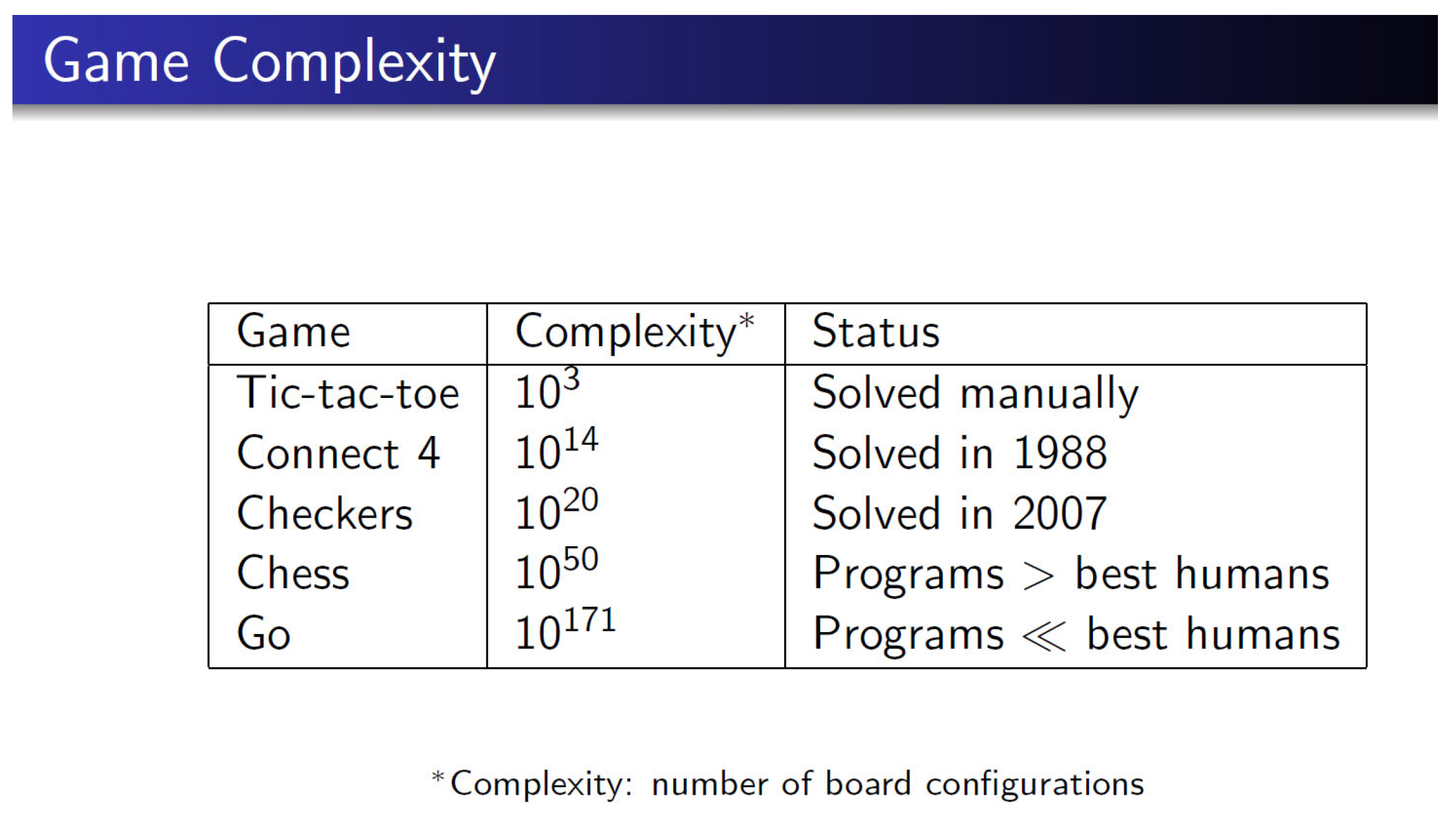
However, the number of possible arrangements of checkers in a heat regenerator could be very high. Thus, finding the optimal arrangement of checkers, of possibly different types, in a heat regenerator could be difficult. In fact, when there are
different types of checkers that can be selected for
each of
positions, the total number of possible arrangements of checkers at
positions is
Thus, for example, when 5 different types of checkers are available for each of the 14 positions, the total number of possible arrangements of checkers, of possibly different types, is
This means that one must evaluate
more than six billion arrangements to reach an optimal arrangement of checkers at 14 positions. Certainly, it seems impractical to solve this optimization problem through this elementary process.
In this article, we will propose an optimization method/algorithm by tree search to tackle this optimization problem. This method is motivated by the recent applications of Artificial Intelligence (AI), based on combination of “Deep Learning” with “Monte-Carlo Tree Search (MCTS)”, to the incredibly complicated board game
Go, Refs. [
16,
17,
18,
19,
20,
21,
22,
23,
24,
25,
26,
27,
28,
29,
30,
31,
32,
33,
34,
35,
36,
37,
38,
39,
40,
41,
42,
43,
44,
45].
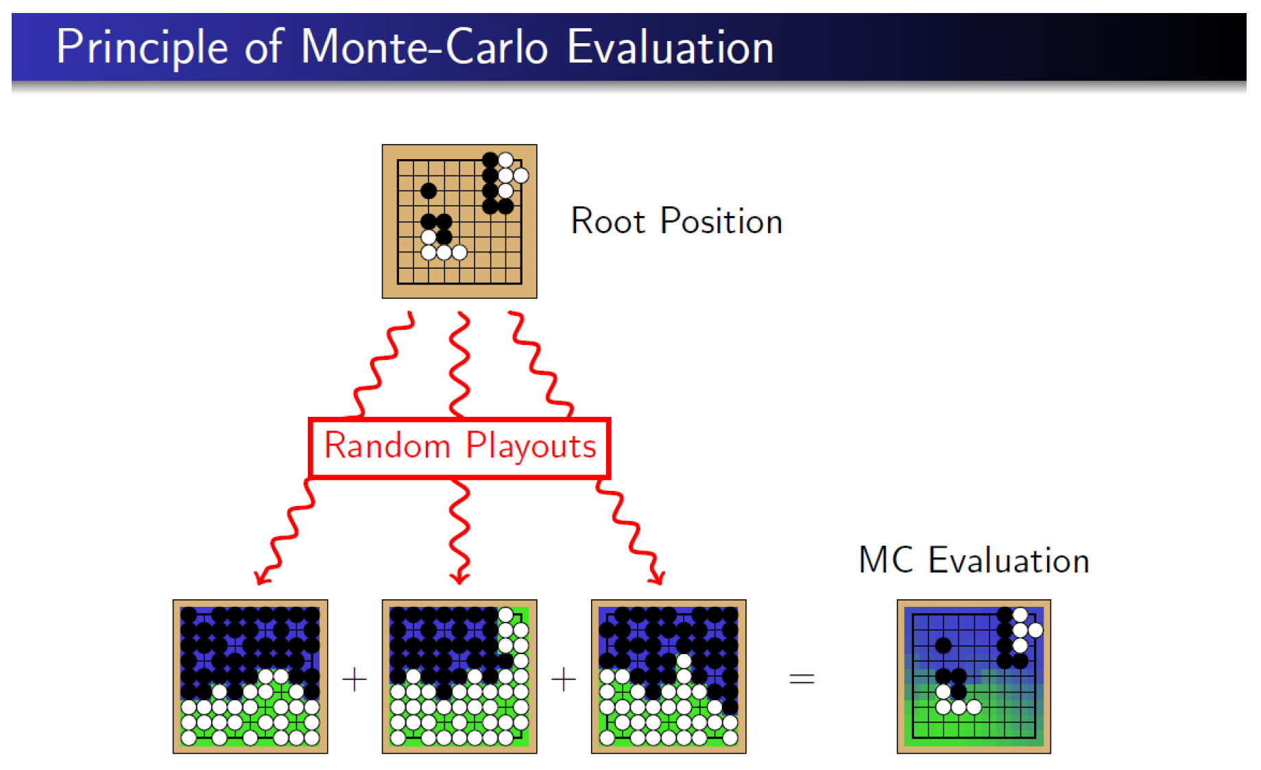
The statistical “Monte-Carlo Method” was proposed in 1949, Ref. [
46], to calculate the area of a region, based on
Random Sampling, to solve problems in
statistical physics. According to the mathematical principle “
Law of Large Numbers”, Refs. [
47,
48,
49], one should be able to estimate, with statistical accuracy, the genuine area of a region when the sampling number is
large enough. By the way, other probabilistic methods “
Stochastic Integrals”, Refs. [
50,
51], based on the Central Limit Theorem, were applied to mathematical finance, Ref. [
52], in those decades.
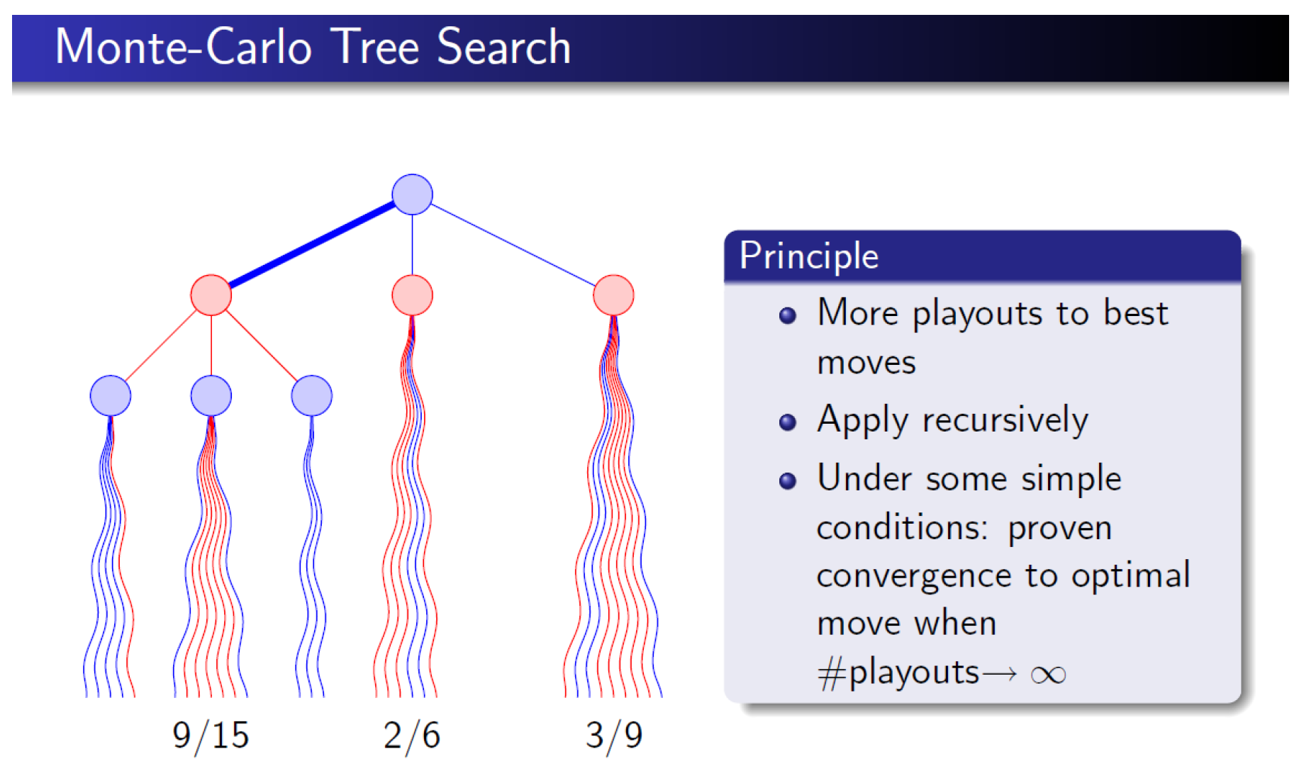
In 1987, B. Abramson applied the “Monte-Carlo Method” to certain “Two-Player Games”: tic-tac-toe, Othello and Chess, Ref. [
16]. B. Abramson proposed the “Expected-Outcome model”, based on the statistical data of “
random game playouts to the end”, as the basis of strategies for a game player. B. Brügmann considered the applications of the “Monte-Carlo Method” to the board game “
Go” in 1993, but not seriously, Ref. [
17]. In 2006, inspired by many predecessors, R. Coulom seriously considered the applications of the “Monte-Carlo Method” to the search tree for the board game “
Go”, Ref. [
18]. See Ref. [
19] for similar work by Kocsis and Szepesvári. The decision-making algorithm proposed in Ref. [
18] was named “Monte-Carlo Tree Search (MCTS)” by R. Coulom. More modifications and improvements, Refs. [
20,
21,
22,
23,
24,
25,
26], were made for MCTS in light of the important contributions by Kocsis and Szepesvári, Ref. [
19], and by Coulom, Ref. [
18]. The MCTS algorithm was also applied to certain games, Refs. [
27,
28,
29,
30,
31]. By combining MCTS with
reinforcement learning based on CNNs (Convolutional Neural Networks), the computer Go player
AlphaGo, developed by Google DeepMind, defeated Lee, Sedol, one of the most brilliant Go players, in a five game Go match in 2016. See Refs. [
32,
33] for further details.
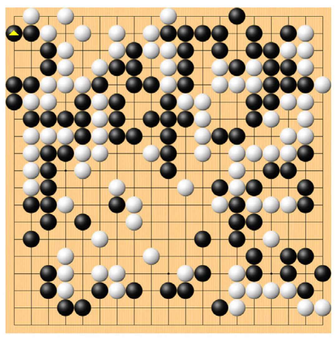
The following three pictures (
Figure 1,
Figure 2 and
Figure 3) were taken from Ref. [
34], which can be found on the website of Rémi Coulom. We sincerely thank Professor Rémi Coulom for kindly granting us permission to use his explanatory pictures in this article. A figure for the board game
Go is shown in
Figure 4.
In 2017, Google DeepMind added a new ingredient “
Dirichlet noise” to
AlphaGo Zero to encourage further exploration by MCTS, which could have been omitted by the earlier versions of
AlphaGo because of low prior probabilities. This deepened the MCTS reinforcement learning of
AlphaGo Zero.
AlphaGo Zero is considered as a genuine AI because
AlphaGo Zero is able to explore the board game Go by MCTS without human knowledge (experience), Ref. [
35]. Applications of Artificial Intelligence with MCTS to other games were developed in Refs. [
36,
37,
38,
39]. Artificial Intelligence with MCTS was also applied to chemical syntheses of organic compounds, Ref. [
40]. Application of MCTS to floor plans was considered in Ref. [
41]. More applications of MCTS are still being explored, Refs. [
42,
43]. For a recent review of MCTS, see Ref. [
44].
Empirical evidence shows that this simple tree search method/algorithm leads to
fast convergence of an optimization search and successfully suggests the
most efficient arrangement of heat-storage ceramic bricks (with the highest long-term Waste Heat Recovery Ratio). See
Section 3 for the details. Thus, this simple tree search method/algorithm may effectively enhance the thermal efficiency of a regenerative combustion system.
2. Materials and Methods
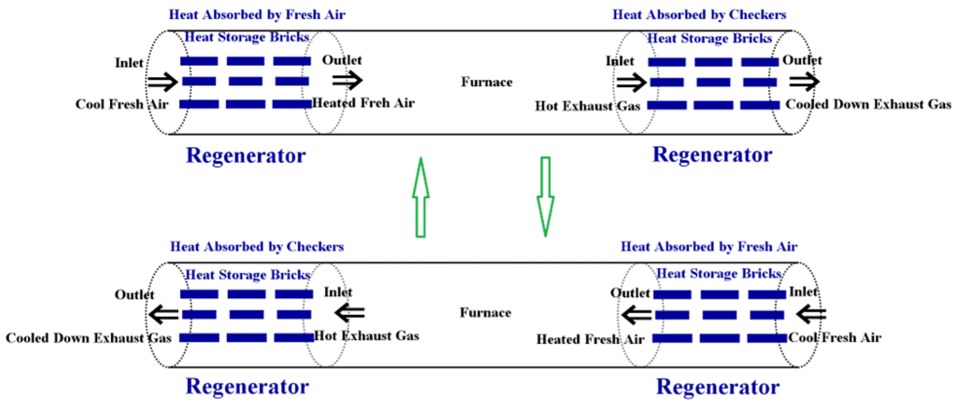
Usually two fixed-bed heat regenerators are utilized in pairs with a central furnace to form a regenerative combustion system. See
Figure 5 for further details. In each heat regenerator, checkers are arranged. The regenerative combustion system operates periodically with a two-phase cycle. The checkers arranged in the heat regenerators, on both ends of a regenerative combustion system, are used to absorb
heat from the high temperature
exhaust gas expelled from the central furnace.
In Phase 1, the cool fresh air flows into the left heat regenerator and is preheated by the checkers arranged there. (The checkers arranged in the left heat regenerator are designed to periodically absorb heat from the high-temperature exhaust gas expelled from the central furnace in Phase 2.) The preheated fresh air then flows into the central furnace for combustion with natural gas. After combustion with natural gas, the high temperature exhaust gas, expelled from the central furnace, then flows into the right heat regenerator and heats up the checkers arranged there. Then Phase 2 starts at the Phase Switch point. In Phase 2, the above process is reversed. The cool fresh air flows into the right heat regenerator and is preheated by the checkers arranged there, which have already absorbed heat from the high-temperature exhaust gas expelled from the central furnace during Phase 1. Then the preheated fresh air flows into the central furnace for combustion with natural gas. Finally, the high-temperature exhaust gas, expelled from the central furnace, flows into the left heat regenerator and heats up the checkers arranged there. Then Phase 1 starts again at the Phase Switch point. A new cycle of operations follows.
2.1. Our Optimization Method/Algorithm by Tree Search
Motivated by the principles of MCTS, we will introduce a simple tree search method/algorithm to find the “
optimal” arrangement, with the
largest long-term
Waste Heat Recovery Ratio (%):
of heat-storage ceramic bricks (checkers) in a heat regenerator, when there are
different types of checkers that can be selected for
each of the
positions in a fixed-bed heat regenerator. In our following discussions, a
node of search tree simply represents an
arrangement of checkers at
positions in a fixed-bed heat regenerator.
We begin with the notion of a “
Partition” of the set
of positions, to be placed by checkers, in a fixed-bed heat regenerator. A
Partition of
is a subset of
such that the largest integer
must be included in
.
Example 1. For the set , and are Partitions of . Assume that
is a Partition of . Using the positive integers in , we may create the following decompositionfor ,
in which Example 2. For the Partition of the set , we have the following decomposition
For the Partitionof the , we will conveniently say that each is an “Interval Component” of with respect to , because each contains certain consecutive positive integers taken from . This phenomenon is clear from the example (Example 2) shown above. We have the following simple facts about the decomposition (2) of .
Fact A. The endpoints of the Interval Components in (2) simply constitute the Partition set of .
Fact B. The Interval Components of the decomposition (2) of , with respect to the Partition , are disjoint.
Fact C. Elements of the Interval Components of the decomposition (2) of are linearly ordered.
There is a
Partial Ordering on the collection of all
Partitions of
. For Partitions
and
of
, we say that
is
finer than
if and only if
We say that
is
strictly finer than
if and only if
We will use the notation
to indicate the condition that
is
strictly finer than
.
Example 3. For Partitions and of , we have .
Now we discuss the notion of “qualified arrangements with respect to a Partition”. Assume that is a Partition of as shown in (1). We say that an arrangement of checkers on is a “qualified arrangement with respect to the Partition ” if and only if the following condition (4) is satisfied.
Definition 1. We say that an arrangement of checkers on is a “qualified arrangement with respect to the Partition ” if the following condition is satisfied.
For each Interval Component of in decomposition (2) with respect to Partition,
Let
denote the class of all “
qualified arrangements with respect to the
Partition ”. Let
denote the norm (the total number of
qualified arrangements with respect to
) of
. Then we have
in which
is the norm (number of elements) of
, as shown in (1).
Example 4. For the Partition of , the total number of “qualified arrangements with respect to the Partition ” is
For the Partition , the total number of “qualified arrangements with respect to the Partition ” is
However, the number of all possible arrangements of checkers on is
.
For Partitions and of , we have the following important.
Fact D. For Partitions and of satisfying , we have
Thus any “qualified arrangement of checkers with respect to Partition ” is naturally a “qualified arrangement of checkers with respect to the Partition ”. Besides, the class o
f arrangements is strictly larger than the class of arrangements. To
initialize a search tree for the optimal (most efficient) arrangements of checkers in a heat regenerator, when
different types of checkers are available for selection at
each of
positions in the heat regenerator, we must choose a
strictly increasing sequence
of
Partitions of
. Let
denote the class of all “
qualified arrangements with respect to the
Partition ”. Then, according to Fact D, the sequence of classes
of arrangements corresponding to the strictly increasing sequence
of Partitions, is naturally
strictly increasing.
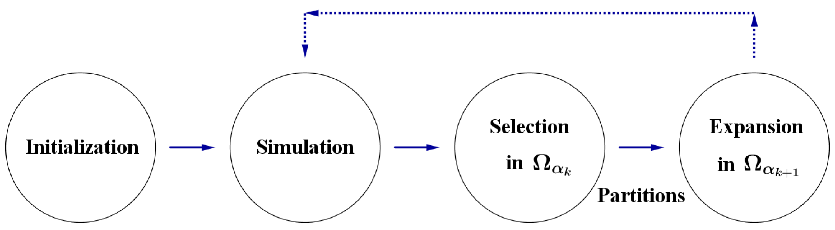
In our tree search, each
arrangement of checkers on
will be considered as a “
node” in the search tree. At the initial stage
, we evaluate the efficiency of each of the arrangements in
(“
qualified arrangements with respect to the
Partition ”) by numerical
Simulation. Then we
select the top
arrangements in
as the “
mother (root) nodes” in
. These selected “mother (root) nodes” will be used to create “
child nodes” (
qualified arrangements with respect to the
Partition ) in
. This process is the
Expansion operator of our algorithm. Then we evaluate the efficiency of each of the
child nodes, created by the
Expansion operator, in
by numerical
Simulation. See
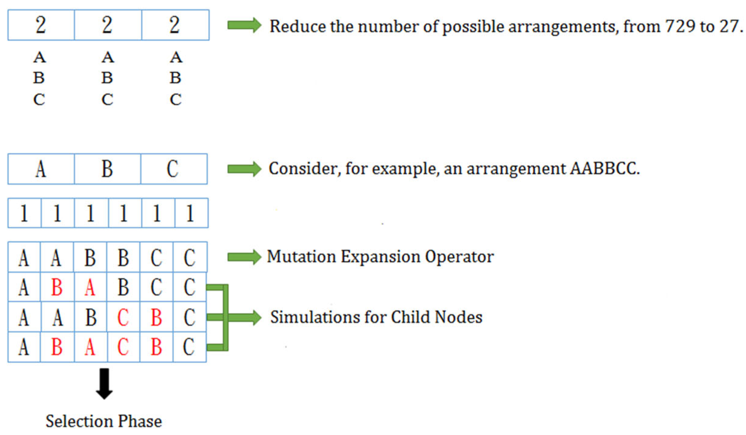
Figure 6 for the phases of our tree search.
In the
Expansion phase of
Figure 6, The “mother (root) nodes” selected in
will be used to
create “child nodes” in
.
2.2. The Expansion Operators
We will discuss two Expansion operators, “Gradient Expansion operator” and “Mutation Expansion operator”, for our tree search method.
We consider the following typical case. Assume that
and
are Partitions of
satisfying
Then, based on
Fact D, we have
Let
be the decomposition of
into a union of
Interval Components with respect to the Partition
. Assume that
. Since
, we note that, for
each Interval Component
, only checkers of the
same type are placed on
by the arrangement
. We assume that, on the Interval Component
, the
checkers arranged by
are all of the type
Assume that
is a “
qualified arrangement with respect to the
Partition ”. Assume that, on the Interval Component
, the checkers arranged by
are all of the type
We say that the arrangement
of checkers is a “
child-node” of
in
, by the “
Gradient Expansion operator”, if the following GE Condition is satisfied.
GE (Gradient Expansion) Condition. There is a sequence of positive integers taken from , satisfying
such thatFor each, we havefor the arrangements and
of checkers on the pair
of adjacent Interval components and .
Besides, outside these pairs of adjacent Interval components, , we have Example 5. For the Partitions and of , we have
These are the decompositions of into unions of Interval Components respectively with respect to the Partitions and .
Assume that we have two different types of checkers and .
Thenis a qualified arrangement of checkers with respect to the Partition .
When is considered as a qualified arrangement with respect to the Partition , it has the following child-nodesby the “Gradient Expansion operator”.
This “
Gradient Expansion operator” is motivated by the usual
Gradient Descent method adopted in
Machine Learning. See, Ref. [
45], for examples. Search through the simple
Gradient Descent method usually converges
slowly. (To expedite the training process of AI, Stochastic Gradient Descent was introduced. See Ref. [
45].)
Now we discuss the “Mutation Expansion operator” under the assumptions (9) to (12). We say that the arrangement of checkers is a “child-node” of in , by the “Mutation Expansion operator”, if the following ME Condition is satisfied.
ME (Mutation Expansion) Condition. There is a sequence of positive integers taken from , satisfying
such thatFor each , we havefor the arrangements and of checkers on the pair of adjacent Interval components and .
Besides, outside these pairs of adjacent Interval components, , we have Example 6. For the Partitions and of , we have the following decompositions
of
into unions of Interval Components, respectively, with respect to Partitions and .
Assume that we have two different types of checkers and .
Then
is a
qualified arrangement of checkers with respect to the Partition .
When is considered as a qualified arrangement with respect to the Partition , it has the following child-nodesby the “Mutation Expansion operator”.
This “
Mutation Expansion operator” is motivated by the
Differential Evolution method. See, for example, Refs. [
53,
54,
55,
56]. A search through this “
Mutation Expansion operator” usually leads to
rapid convergence. Thus, we may use “tree search through the
Mutation Expansion operator” to help us to find a satisfactory strictly increasing sequence
of
Partitions of
. Then we may use this proper strictly increasing sequence of
Partitions of
to execute a delicate “tree search through the
Gradient Expansion operator”, which usually converges slowly.
2.3. The Numerical Simulation Methods
To speed up the evaluation process for an arrangement of checkers in a fixed-bed heat regenerator, our numerical simulations are based on simplified 1-dimensional partial differential equations as in Refs. [
1,
2,
3]. This 1-dimensional model has been discussed in Refs. [
11,
15,
57]. (See Ref. [
58] for the fundamental theory of Continuum Mechanics.) These 1-dimensional partial differential equations were further developed in Refs. [
4,
5].
Let us consider the two-phase cycle of a fixed-bed heat regenerator, which is placed on the
right end of a regenerative combustion system, as shown in
Figure 7. In Phase 1, the high-temperature exhaust gas, from the central furnace, flows into the
right heat regenerator and
heats up the
checkers arranged there. Then Phase 2 starts at the
Phase Switch point of time. In Phase 2, the above process is
reversed. The cool fresh air flows into the
right heat regenerator and is
preheated by the
checkers arranged there, which already absorbed heat from the high-temperature exhaust gas expelled from the central furnace during Phase 1. Then the
preheated fresh air flows into the central furnace for combustion with natural gas.
Let
denote the
switch time of the operation cycle of the fixed-bed heat regenerator shown above. Thus
is the
period of the operation cycle. When
, Phase 1 operates. When
, Phase 2 operates. To evaluate the efficiency of an arrangement of checkers on a fixed-bed heat regenerator, this operation cycle must be performed periodically until we reach an approximately
steady state. We assume that the fixed-bed heat regenerator is located on the interval
of the
-axis. See
Figure 7 for details.
We use the subscript
ar to indicate functions related to the
fresh air flow. We use the subscript
ex to indicate functions related to the
exhaust gas flow. We use the subscript
s to indicate functions related to the
checkers (solid porous medium). Let
be a nonnegative integer. When
we have the following 1-dimensional partial differential equations:
and
satisfying the following boundary conditions
Remark 1. Here, in (21) and (22), we omit the Darcy dissipation. The Darcy dissipation may be estimated through experiments or through the Ergun equation for the pressure drop. See page 86 of Refs. [11,15,57] for a discussion of the Ergun equation. See, for examples, Refs. [59,60] for certain experimental investigations on the pressure drop. For the fluid flows (fresh air or exhaust gas) considered in our simulations, we have In the CFD simulations on Ansys Fluent by W.-J. Syu, Ref. [10], it is found that, for the following arrangement of checkersat 6 positions in a fixed-bed heat regenerator, the pressure drop isThe material parameters of these checkers, considered above, are listed in Table 1 below. It should be pointed out that the CFD simulations on Ansys Fluent by W.-J. Syu, [10], are found to be compatible with the experimental results provided by the Metal Industries Research & Development Centre (MIRDC) of Taiwan. Thus, for arrangements of 6 checkers, whose material parameters are not too far from those shown above, it is reasonable to omit the Darcy dissipation in our numerical simulations. In fact, experimental data of MIRDC supports this omission in our optimization search. See Section 3 for a comparison of our 1-dimensional numerical simulations with the experimental results provided by MIRDC. When
, we have the following 1-dimensional partial differential equations:
and
satisfying the following boundary conditions
Here
is the superficial flow velocity of the gas/air.
and
are, respectively, the densities of the gas/air and the solid porous medium (checkers).
and
are, respectively, the specific heat capacities of the gas/air and the solid porous medium (checkers).
and
are, respectively, the thermal conductivities of the gas/air and the solid porous medium (checkers).
and
are, respectively, the temperatures of the gas/air and the solid porous medium (checkers).
is the void fraction (
porosity) of the solid porous medium (checkers).
is the specific surface area of the porous ceramic medium (checkers) exposed to gas/air per unit volume.
is the
heat transfer coefficient of the solid porous medium (checkers).
is the
heat dissipation through the
external surface of a fixed-bed heat regenerator. We assume that
.
We have the following relation for the Nusselt number of the fluid (gas/air) flow:
in which
is the
characteristic length. Let
and
denote, respectively, the Reynolds number and the Prandtl number of the fluid (gas/air) flow. We will use the following classic relation
of Sieder and Tate to calculate the Nusselt number. Here
and
are, respectively, the viscosity of fluid at the mean bulk temperature and the viscosity of fluid at the wall. See page 583 of Ref. [
6]. Note that, for a positive real number
, we have
when
is
not large. Thus, when performing numerical simulations, we will use the simplified formula
Let and be, respectively, the mass flow rates of the exhaust gas flow and of the fresh air flow. Let and be the specific heat capacities of the fresh air, respectively, at the Inlet of fresh air (into the right heat regenerator) and at the Outlet of fresh air (into the central furnace). Let and be the temperatures of the fresh air, respectively, at the Inlet of fresh air (into the right heat regenerator) and at the Outlet of fresh air (into the central furnace). Let be the specific heat capacity of the exhaust gas flow at the Inlet of exhaust gas (into the right heat regenerator). Let be the temperature of the exhaust gas flow at the Inlet of exhaust gas (into the right heat regenerator).
We define the
Waste Heat Recovery Ratio (%) of an arrangement of checkers in a fixed-bed heat regenerator as follows:
We use the long-term Waste Heat Recovery Ratio to evaluate the efficiency of an arrangement of checkers in a fixed-bed heat regenerator.
To expedite the process of simulations, we use the following polynomials in our simulations.
These polynomials are derived based on the data provided in the Appendices of Ref. [
7] at
Atmospheric Pressure. For the densities of the air/gas, we use the following polynomial
in our simulations. This polynomial is derived based on the data for air provided in the Appendices of Ref. [
7] at
Atmospheric Pressure.
3. Results
Before starting our optimization process using the tree search, we test the validity of our 1-dimensional partial differential equations. This 1-dimensional model has been discussed in Refs. [
11,
15,
57]. It has also been utilized in Refs. [
1,
2,
3,
4,
5]. We test our 1-dimensional modeling for two types of checkers, Cordierite and Mullite, with the material parameters shown in
Table 1 of
Section 2. We consider the following arrangement of checkers
at 6 positions in a fixed-bed heat regenerator.
These checkers are provided by the Metal Industries Research & Development Centre (MIRDC) of Taiwan. It is known that the CFD simulations on Ansys Fluent by W.-J. Syu, [
10], are compatible with the experimental results of MIRDC. Thus, it is natural to compare our 1D simulations with the 3D CFD simulations on Ansys Fluent for the arrangement of checkers described above.
We assume that the temperature of exhaust gas, expelled from the central furnace, is 900 °C (1173.15 K). We assume that the temperature of fresh air, at the Inlet, is 40 °C (313.15 K). We assume that the time of the Phase Switch is . We assume that the superficial flow velocity of the exhaust gas is . We assume that the superficial flow velocity of the fresh air is .
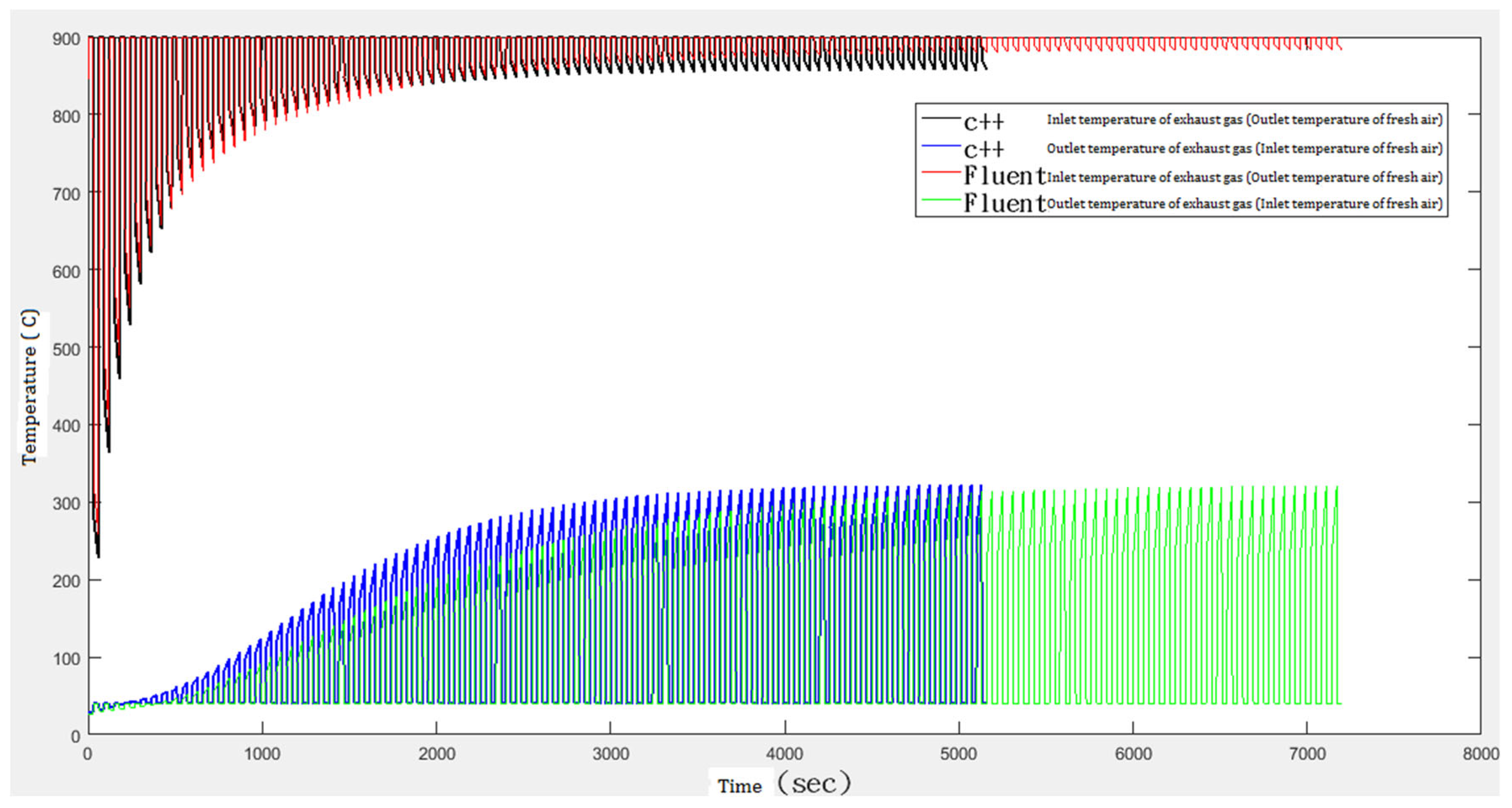
The comparison of our 1D simulations with the 3D CFD simulations on Ansys Fluent for the arrangement of checkers
at 6 positions, in a fixed-bed heat regenerator, is shown in
Figure 8.
In
Figure 8, the Inlet temperature of exhaust gas (expelled from the central furnace) and the Outlet temperature of fresh air (into the central furnace), based on our 1D simulations using C++, is shown in black. In
Figure 8, the Inlet temperature of exhaust gas (expelled from the central furnace) and the Outlet temperature of fresh air (into the central furnace), based on 3D CFD simulations on Ansys Fluent, is shown in red.
In
Figure 8, the Outlet temperature of exhaust gas (expelled from the right heat regenerator) and the Inlet temperature of fresh air (into the right heat regenerator), based on our 1D simulations using C++, is shown in blue. In
Figure 8, the Outlet temperature of exhaust gas (expelled from the right heat regenerator) and the Inlet temperature of fresh air (into the right heat regenerator), based on 3D CFD simulations on Ansys Fluent, is shown in green.
It can be observed that, in the
long term, our numerical simulation results, based on the 1-dimensional partial differential equations, are consistent with the simulation results based on CFD (Computational Fluid Dynamics) on
Ansys Fluent. See
Figure 8.
We also test the validity of our 1-dimensional model by comparing our simplified 1-dimensional numerical simulation results with the experimental results provided by the Metal Industries Research & Development Centre (MIRDC) of Taiwan. There are 3 types of checkers,
A,
B and
C, used in an arrangement
of checkers at 13 positions. The material parameters of these 3 types of checkers,
A,
B and
C, are shown in
Table 2.
There are two experiments provided by MIRDC. The operating parameters for Experiments 1 and 2 are shown in
Table 3. The
Phase Switch time is
for both experiments. The superficial flow velocity of the exhaust gas is
. The superficial flow velocity of the fresh air is
.
A comparison of our simplified 1-dimensional numerical simulation results, in the
long term, with the experimental results of MIRDC is shown in
Table 4.
It can be observed through
Table 4 that, in the long term, our numerical simulation results, based on the 1-dimensional model, are compatible with the experimental results of MIRDC.
Now we apply our simple tree search method with the Mutation Expansion operator to solve the optimization problem for 3 types of checkers to be arranged at 6 positions in a fixed-bed regenerator. The material parameters of these 3 types of checkers,
A,
B and
C, are shown in
Table 2. These checkers are provided by MIRDC. The operating parameters for a regenerative combustion system with two fixed-bed heat regenerators are shown in
Table 3.
Thus, we have
. We choose the
strictly increasing sequence
of
Partitions of
. Thus, we have the following decomposition
of
into a union of
Interval Components
with respect to the Partition
.
We select the top 15 arrangements in as the “mother (root) nodes” in to create “child nodes” (qualified arrangements with respect to the Partition ) in .
For a
complete evaluation process for the total
possible arrangements of checkers, based on 1D simulations, it takes 63 h to finish this evaluation process. The top 3 arrangements are shown in
Table 5.
For the optimization process by our simple
tree search method, it takes only 6 h to evaluate
possible arrangements of checkers, based on 1D simulations. The top three arrangements, found by this simple
tree search method, are shown in
Table 6.
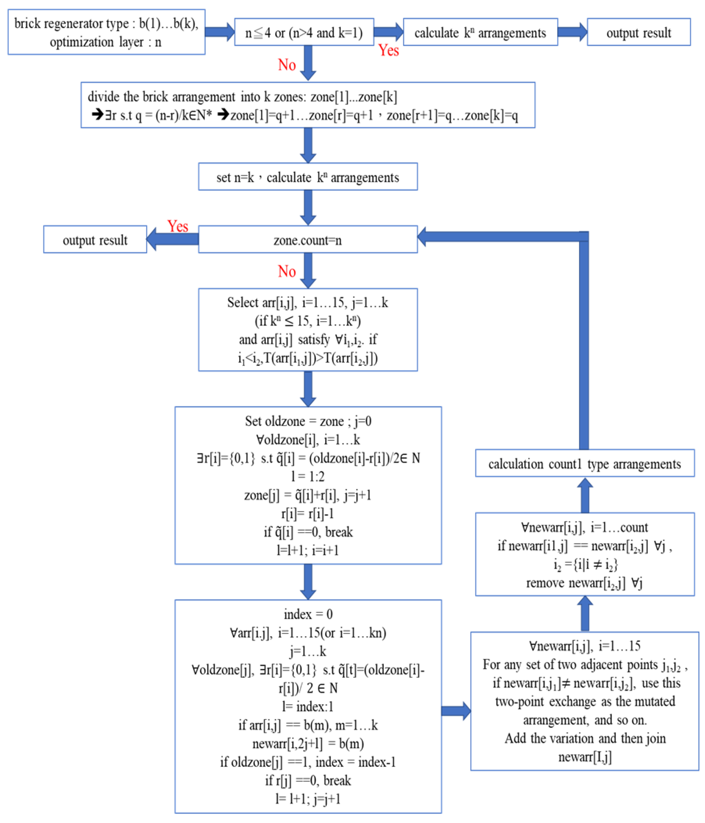
An outline for our tree search method is shown in
Figure 9.
Thus, empirical evidence shows that our
tree search method is helpful and
efficient. An algorithm based on our simple tree search method, with the Mutation Expansion operator, is shown in
Figure 10.
5. Conclusions
In this article, we propose an optimization method using tree search to enhance the thermal efficiency of a regenerative combustion system by searching the optimal arrangements of heat-storage ceramic bricks with the highest long-term Waste Heat Recovery Ratio.
To examine this method, we consider arrangements of heat-storage ceramic bricks at 6 positions. We use the checkers provided by MIRDC of Taiwan.
To expedite the search process, we use simplified 1D simulations to replace 3D CFD simulations on Ansys Fluent. We test the validity of our simplified 1D model by comparing our 1D simulation results, in the long term, with the experimental results of MIRDC. Empirical evidence shows that our simplified 1D model can be trusted.
We then use our simple tree search method/algorithm with simplified 1D simulations to search the arrangements, of heat-storage ceramic bricks at 6 positions, with the highest long-term
Waste Heat Recovery Ratio. A
complete evaluation of the total
possible arrangements of checkers, based on 1D simulations, takes 63 h to finish this evaluation process. For our simple
tree search method/algorithm, it takes only 6 h to find the
most efficient arrangement, of heat-storage ceramic bricks at 6 positions, with the highest long-term Waste Heat Recovery Ratio.
Empirical evidence shows that this simple tree search method/algorithm leads to fast convergence of an optimization search and successfully suggests the most efficient arrangement of heat-storage ceramic bricks (with the highest long-term Waste Heat Recovery Ratio). Thus, this simple tree search method/algorithm may effectively enhance the thermal efficiency of a regenerative combustion system.


