
An Interpretable Method for Anomaly Detection in Multivariate Time Series Predictions


Abstract
1. Introduction
2. Related Works
3. Interpretable Method Design
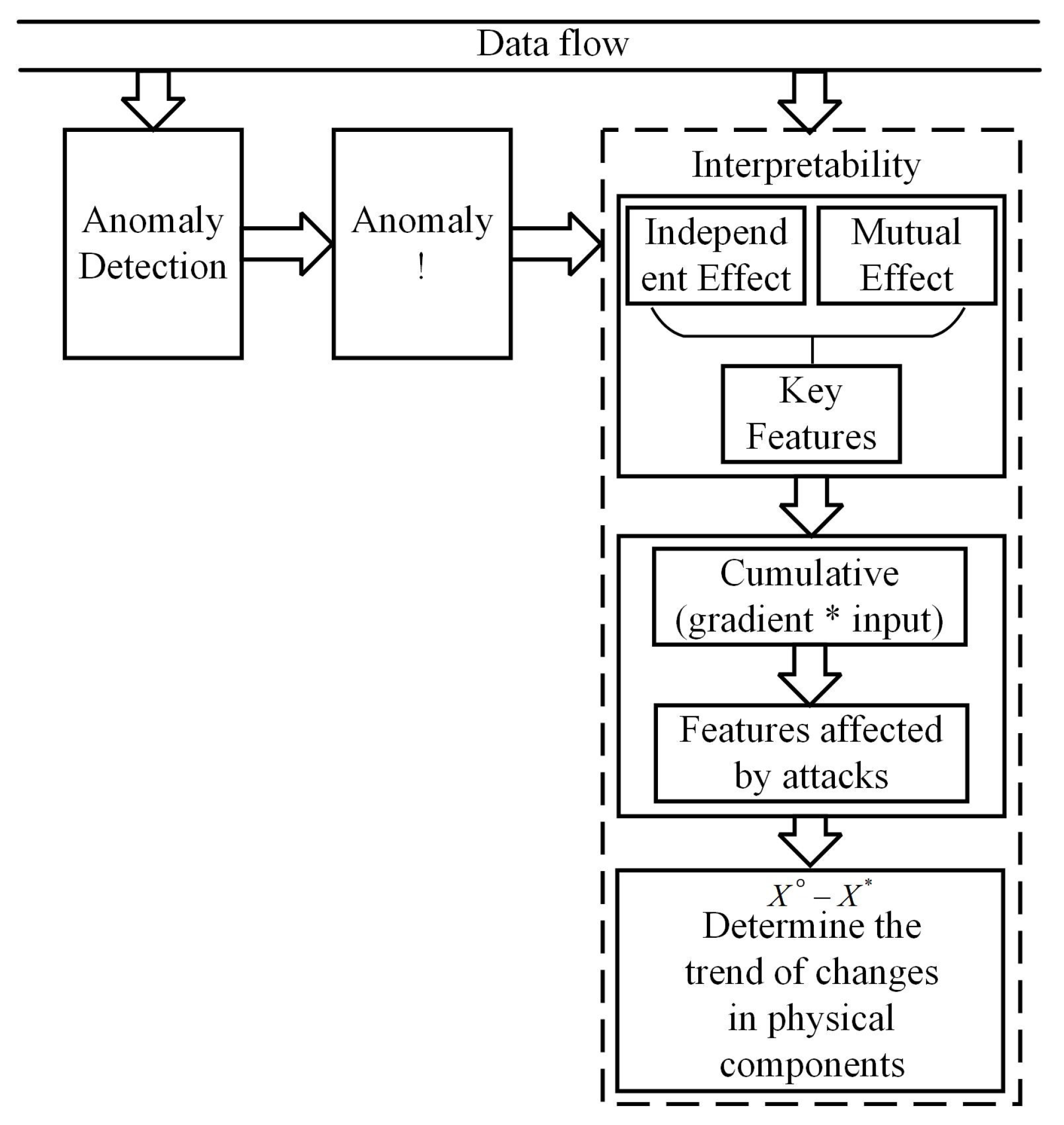
3.1. Scheme Framework
3.2. Detailed Design
3.3. Iteration Process for the Optimization Algorithm
| Algorithm 1: The Proposed Interpretable Algorithm |
Input: Data (containing one or more abnormal input samples ), maximum iteration times Output: Interpretation result, i.e., trend of feature changes affected by attacks
|
4. Experiments
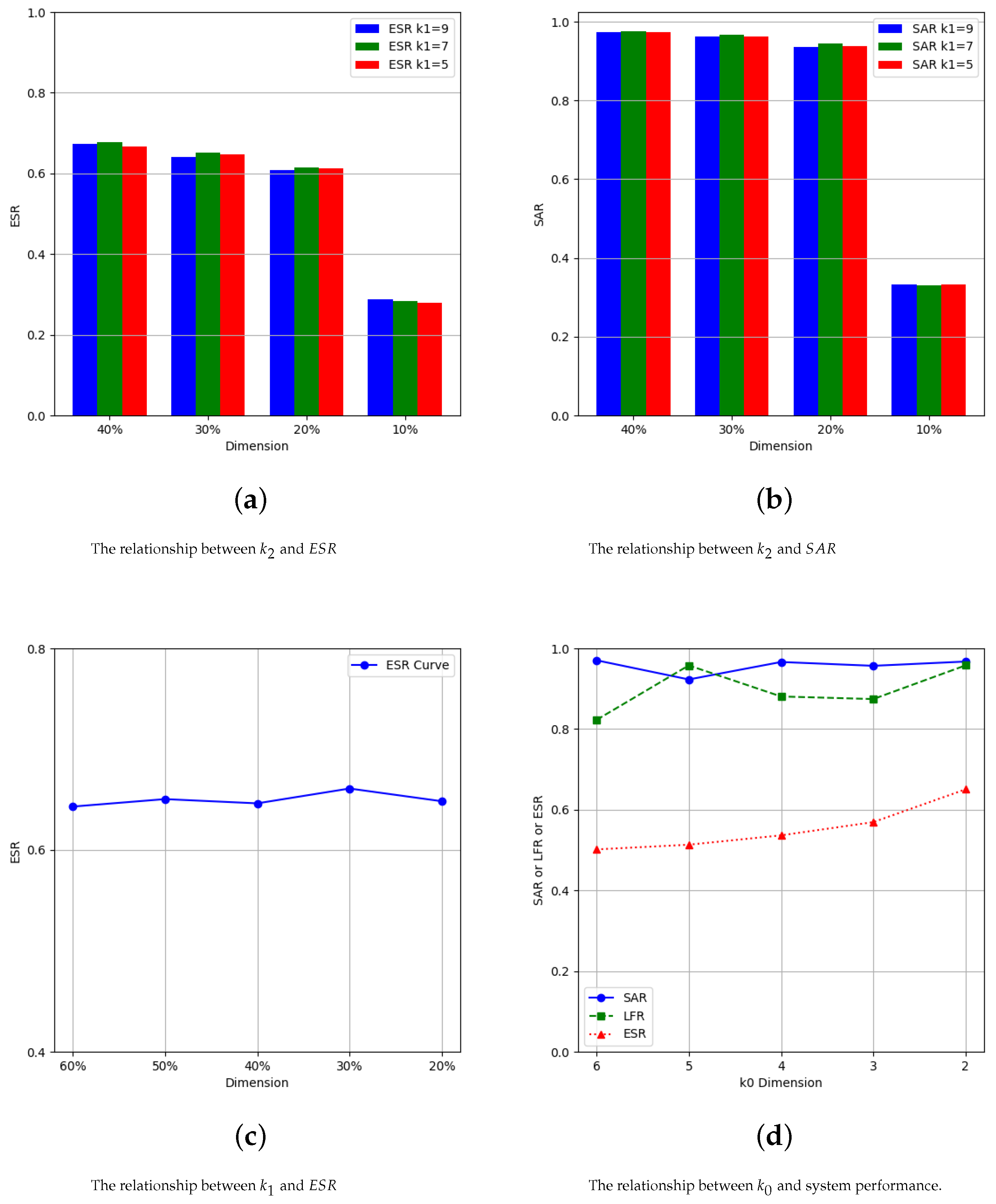
4.1. Parameter Settings
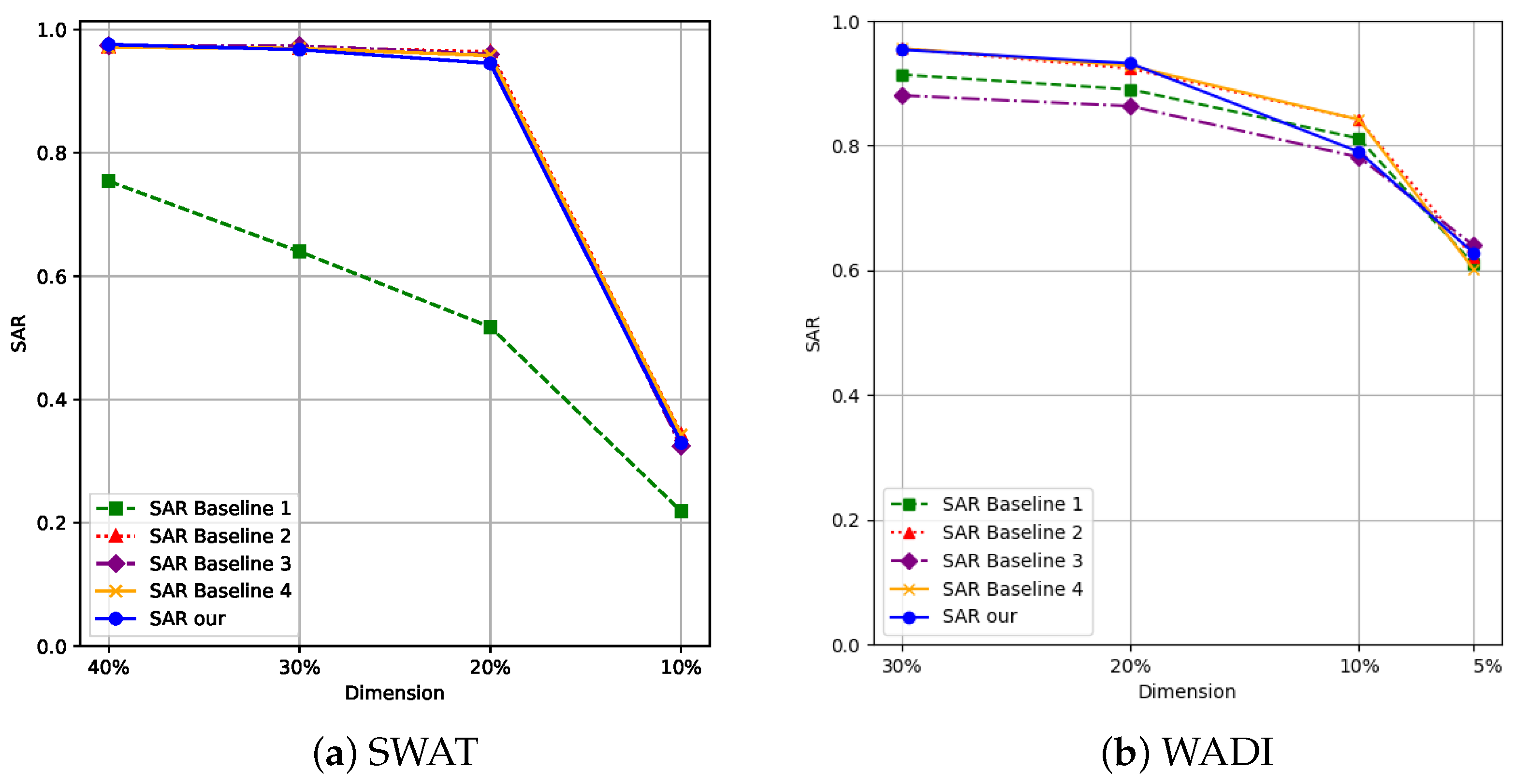
4.2. Algorithm Performance Comparisons
5. Summary
Author Contributions
Funding
Institutional Review Board Statement
Data Availability Statement
Acknowledgments
Conflicts of Interest
References
- Hassija, V.; Chamola, V.; Mahapatra, A.; Singal, A.; Goel, D.; Huang, K.; Scardapane, S.; Spinelli, I.; Mahmud, M.; Hussain, A. Interpreting black-box models: A review on explainable artificial intelligence. Cogn. Comput. 2024, 16, 45–74. [Google Scholar] [CrossRef]
- Yu, A.; Yang, Y.B. Learning to explain: A gradient-based attribution method for interpreting super-resolution networks. In Proceedings of the ICASSP 2023-2023 IEEE International Conference on Acoustics, Speech and Signal Processing (ICASSP), Rhodes Island, Greek, 4–10 June 2023; pp. 1–5. [Google Scholar]
- Li, Z.; Zhu, Y.; Van Leeuwen, M. A survey on explainable anomaly detection. Acm Trans. Knowl. Discov. Data 2023, 18, 1–54. [Google Scholar] [CrossRef]
- Xu, L.; Wang, B.; Zhao, D.; Wu, X. DAN: Neural network based on dual attention for anomaly detection in ICS. Expert Syst. Appl. 2025, 263, 125766. [Google Scholar] [CrossRef]
- Moustafa, N.; Koroniotis, N.; Keshk, M.; Zomaya, A.Y.; Tari, Z. Explainable intrusion detection for cyber defences in the internet of things: Opportunities and solutions. IEEE Commun. Surv. Tutor. 2023, 25, 1775–1807. [Google Scholar] [CrossRef]
- Zhang, Y.; Tiňo, P.; Leonardis, A.; Tang, K. A survey on neural network interpretability. IEEE Trans. Emerg. Top. Comput. Intell. 2021, 5, 726–742. [Google Scholar] [CrossRef]
- Carletti, M.; Masiero, C.; Beghi, A.; Susto, G.A. Explainable machine learning in industry 4.0: Evaluating feature importance in anomaly detection to enable root cause analysis. In Proceedings of the 2019 IEEE international conference on systems, man and cybernetics (SMC), Bari, Italy, 6–9 October 2019; pp. 21–26. [Google Scholar]
- Sundararajan, M.; Taly, A.; Yan, Q. Axiomatic attribution for deep networks. In Proceedings of the International Conference on Machine Learning, Sydney, Australia, 6 August 2017; pp. 3319–3328. [Google Scholar]
- Han, X.; Cheng, H.; Xu, D.; Yuan, S. InterpretableSAD: Interpretable Anomaly Detection in Sequential Log Data, Sydney. In Proceedings of the 2021 IEEE International Conference on Big Data, Chengdu, China, 24–26 April 2021; pp. 1183–1192. [Google Scholar]
- Sipple, J. Interpretable, multidimensional, multimodal anomaly detection with negative sampling for detection of device failure. In Proceedings of the International Conference on Machine Learning. International Conference on Machine Learning (PMLR), San Francisco, CA, USA, 7 February 2020; pp. 9016–9025. [Google Scholar]
- Yang, R.; Wang, B.; Bilgic, M. IDGI: A framework to eliminate explanation noise from integrated gradients. In Proceedings of the IEEE/CVF Conference on Computer Vision and Pattern Recognition, Vancouver, BC, Canada, 18 June 2023; pp. 23725–23734. [Google Scholar]
- Nguyen, Q.P.; Lim, K.W.; Divakaran, D.M.; Low, K.H.; Chan, M.C. Gee: A gradient-based explainable variational autoencoder for network anomaly detection. In Proceedings of the 2019 IEEE Conference on Communications and Network Security (CNS), Washington, DC, USA, 3–5 June 2019; pp. 91–99. [Google Scholar]
- Jiang, R.Z.; Xue, Y.; Zou, D. Interpretability-aware industrial anomaly detection using autoencoders. IEEE Access 2023, 11, 60490–60500. [Google Scholar] [CrossRef]
- Yang, Y.; Wang, P.; He, X.; Zou, D. GRAM: An interpretable approach for graph anomaly detection using gradient attention maps. Neural Netw. 2024, 178, 106463. [Google Scholar] [CrossRef] [PubMed]
- Kauffmann, J.; Müller, K.R.; Montavon, G. Towards explaining anomalies: A deep Taylor decomposition of one-class models. Pattern Recognit. 2020, 101, 107198. [Google Scholar] [CrossRef]
- Han, D.; Wang, Z.; Chen, W.; Zhong, Y.; Wang, S.; Zhang, H.; Yang, J.; Shi, X.; Yin, X. Deepaid: Interpreting and improving deep learning-based anomaly detection in security applications. In Proceedings of the 2021 ACM SIGSAC Conference on Computer and Communications Security, New York, NY, USA, 15–19 November 2011; pp. 3197–3217. [Google Scholar]
- Liu, Y.; Chen, W.; Zhang, T.; Wu, L. Explainable anomaly traffic detection based on sparse autoencoders. Netinfo Secur. 2023, 23, 74–85. [Google Scholar]
- Kraskov, A.; Stögbauer, H.; Grassberger, P. Estimating mutual information. Phys. Rev. Stat. Nonlinear Soft Matter Phys. 2004, 69, 066138. [Google Scholar] [CrossRef] [PubMed]
- Tang, S.; Ding, Y.; Wang, H. Industrial Control Anomaly Detection Based on Distributed Linear Deep Learning. Comput. Mater. Contin. 2025, 82, 1. [Google Scholar] [CrossRef]
- Lundberg, S.M.; Lee, S.I. A unified approach to interpreting model predictions. Adv. Neural Inf. Process. Syst. 2017, 30. [Google Scholar]
- Ribeiro, M.T.; Singh, S.; Guestrin, C. “Why should i trust you?” Explaining the predictions of any classifier. In Proceedings of the 22nd ACM SIGKDD International Conference on Knowledge Discovery and Data Mining, San Francisco, CA, USA, 13–17 August 2016; pp. 1135–1144. [Google Scholar]

| Parameters | SWAT | WADI |
|---|---|---|
| learning rate | 0.1 | 0.1 |
| Optimization frequency | 100 | 50 |
| 0.7 | 0.7 | |
| 0.005 | 0.005 | |
| 0.001 | 0.001 | |
| K | 3 | 3 |
| 25 | 25 | |
| w | 0.9 | 0.6 |
| 2 | 2 | |
| 7 | 7 | |
| 4 | 4 |
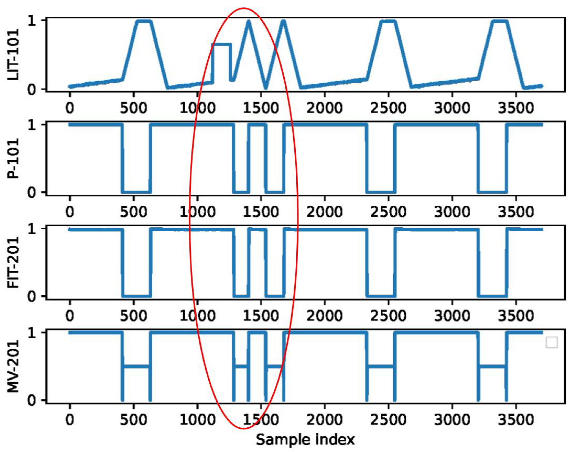
| Attack Index | Features Affected by Attacks | Trend of Changes |
|---|---|---|
| Attack 1, sample 1892 | P-203 | Value increased |
| Attack 1, sample 1892 | FIT-201 | Value increased |
| Attack 1, sample 1892 | LIT-101 | Value decreased |
| Attack 1, sample 1892 | MV-101 | Value increased |
| Attack 30, sample 280322 | MV-101 | Value decreased |
| Attack 30, sample 280322 | P-101 | Value increased |
| Attack 30, sample 280322 | MV-201 | Value increased |
| Attack 30, sample 280322 | P-102 | Value increased |
| (%) | (%) | (%) | |
|---|---|---|---|
| Baseline 1 | 76.45 | 63.99 | 38.75 |
| Baseline 2 | 95.78 | 97.04 | 56.28 |
| Baseline 3 | 76.34 | 97.36 | 45.93 |
| Baseline 4 | 95.78 | 96.94 | 61.67 |
| LIME | - | 66.42 | - |
| SHARP | - | 90.39 | - |
| Our method | 96.73 | 95.78 | 65.05 |
| (%) | (%) | (%) | |
|---|---|---|---|
| Baseline 1 | 56.84 | 81.16 | 57.48 |
| Baseline 2 | 60.82 | 84.18 | 56.94 |
| Baseline 3 | 47.58 | 78.15 | 58.23 |
| Baseline 4 | 60.82 | 84.18 | 56.97 |
| LIME | - | 53.71 | - |
| SHARP | - | 13.02 | - |
| Our method | 60.82 | 79.01 | 57.16 |
Disclaimer/Publisher’s Note: The statements, opinions and data contained in all publications are solely those of the individual author(s) and contributor(s) and not of MDPI and/or the editor(s). MDPI and/or the editor(s) disclaim responsibility for any injury to people or property resulting from any ideas, methods, instructions or products referred to in the content. |
© 2025 by the authors. Licensee MDPI, Basel, Switzerland. This article is an open access article distributed under the terms and conditions of the Creative Commons Attribution (CC BY) license (https://creativecommons.org/licenses/by/4.0/).
Share and Cite
Tang, S.; Ding, Y.; Wang, H. An Interpretable Method for Anomaly Detection in Multivariate Time Series Predictions. Appl. Sci. 2025, 15, 7479. https://doi.org/10.3390/app15137479
Tang S, Ding Y, Wang H. An Interpretable Method for Anomaly Detection in Multivariate Time Series Predictions. Applied Sciences. 2025; 15(13):7479. https://doi.org/10.3390/app15137479
Chicago/Turabian StyleTang, Shijie, Yong Ding, and Huiyong Wang. 2025. "An Interpretable Method for Anomaly Detection in Multivariate Time Series Predictions" Applied Sciences 15, no. 13: 7479. https://doi.org/10.3390/app15137479
APA StyleTang, S., Ding, Y., & Wang, H. (2025). An Interpretable Method for Anomaly Detection in Multivariate Time Series Predictions. Applied Sciences, 15(13), 7479. https://doi.org/10.3390/app15137479