Comparison Between Broadband and Personal Exposimeter Measurements for EMF Exposure Map Development Using Evolutionary Programming

Abstract

In this study, we provide a comparison of radiofrequency electromagnetic field exposure level maps as determined using two approaches: a broadband meter (NARDA EMR-300) equipped with an isotropic probe in the range of 100 kHz to 3 GHz, and a Personal Exposimeter (Satimo EME Spy 140) in the range of 88 MHz to 5.8 GHz. The aim of this research was to determine the necessary adjustments to the measurements made with personal exposimeters to obtain RF-EMF exposure maps equivalent to those made with broadband meters. We evaluated different possibilities to obtain the best equivalence of measurements between both devices. For this purpose, the datasets obtained in both cases were analyzed, as well as the possible correction factors. First, the possibility of establishing a single or double correction factor depending on the existence (or lack thereof) of a line of sight with respect to the base stations was analyzed by minimizing the average value of the error between the values of the broadband meter and the corrected values of the personal exposure meter. Due to the differences observed in the exposure maps, a second procedure was carried out, in which a genetic algorithm was used to determine the ratio between the measurements from both methods (the broadband meter and personal exposure meter), depending on the existence (or lack thereof) of a line of sight, and we compared the exposure maps generated using kriging interpolation.

1. Introduction

Personal exposure to radiofrequency electromagnetic field (RF-EMF) has substantially increased as new wireless technologies are introduced. Society has become more concerned about the possible effects of RF-EMFs on human health in parallel to this increase in exposure. Although recent studies indicate that the available evidence suggests that acute RF-EMFs below regulatory limits do not cause symptoms, concern about this issue continues to grow in the population [1]. Therefore, in addition to monitoring levels, it is necessary to provide results that allow the population to adequately perceive the risk of exposure to RF-EMFs. Geographical interpolation techniques such as kriging allow for the production of exposure maps that are easily understandable by the general public and therefore contribute to the adequate perception of this risk.

Measurements of personal exposure to RF-EMF can be made using personal exposimeters (PEMs) [2], broadband meters (BBMs) [3], or narrowband spectrum analyzers (NBMs). PEMs have been widely used in many different procedures due to their versatility and ease of use, meaning they can be deployed without affecting everyday tasks [4,5,6]. They are also highly useful for the characterization of an individual’s unique exposure and microenvironments [7]. The characterization of exposure with PEMs provides individualized and detailed temporal and spatial information, but such characterization tasks are costly in terms of time and human resources. A BBM is the optimal solution for recording many measurements across a wide area involving various sources (from various locations) or a single source with various frequencies, because BBMs are not as expensive as narrowband measurement devices, and they give a value of the total electric field at that specific point. BBM measurements are adequate to ensure compliance with legal standards; however, BBMs have the disadvantage of being costly in economic terms compared to PEMs, and it is also impossible to identify signal sources based on their frequency [8].

The objective of this study is to compare RF-EMF exposure measurements recorded with a broadband meter and a personal exposimeter in order to develop equivalent exposure maps. This study aims to evaluate the feasibility of adjusting personal exposimeter measurements to match those of broadband meters, thereby providing a more accessible and cost-effective methodology for creating exposure maps that assess RF-EMF risks in urban environments.

The rest of this article is organized as follows. Section 2 describes the equipment and measurement procedures used for data collection, the geographical location of the measurement points taken, and the tools used for their analysis. In Section 3, the measurements taken with the BBM and the PEM are presented, as well as the corrections made with one and two factors and the statistical properties of the ensembles. To find different approximations to the optimal value, an evolutionary algorithm was used. This made it possible to obtain the ranges of variation in the correction factors. The exposure maps generated and the differences between the values generated from the BBM and the PEM, along with their different corrections, are also shown. Finally, Section 4 discusses the limitations of the results and the methodology we employed, and Section 5 presents the conclusions reached.

2. Materials and Methods

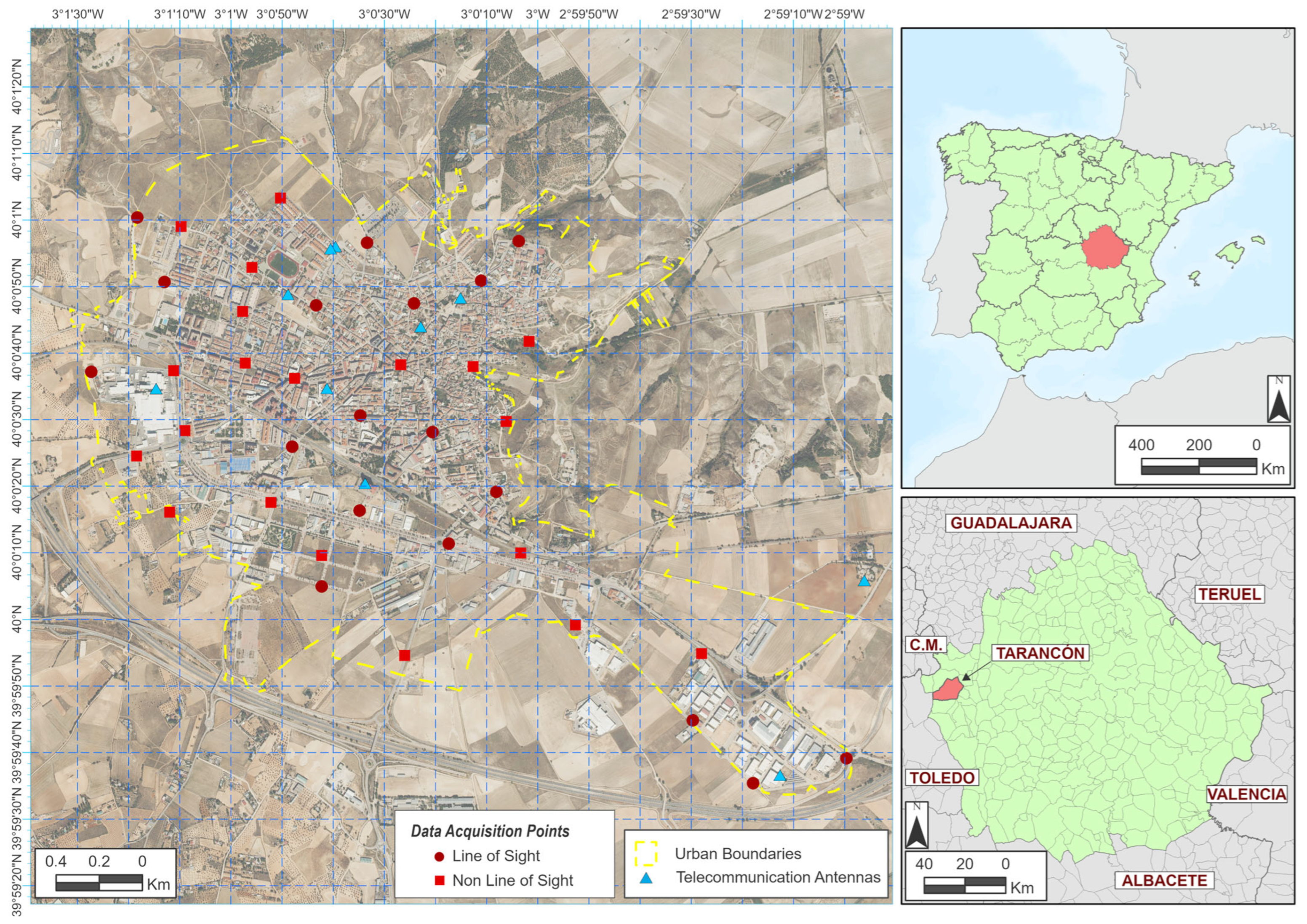
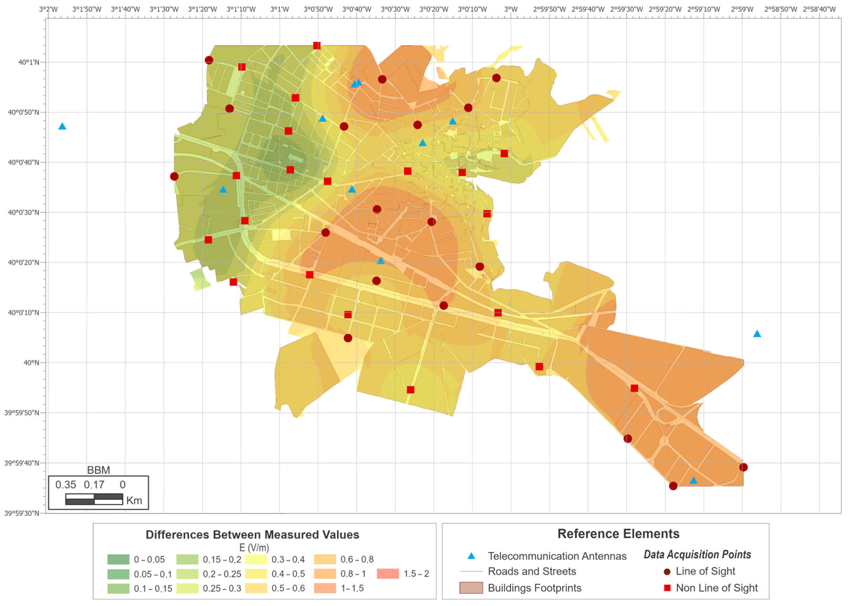
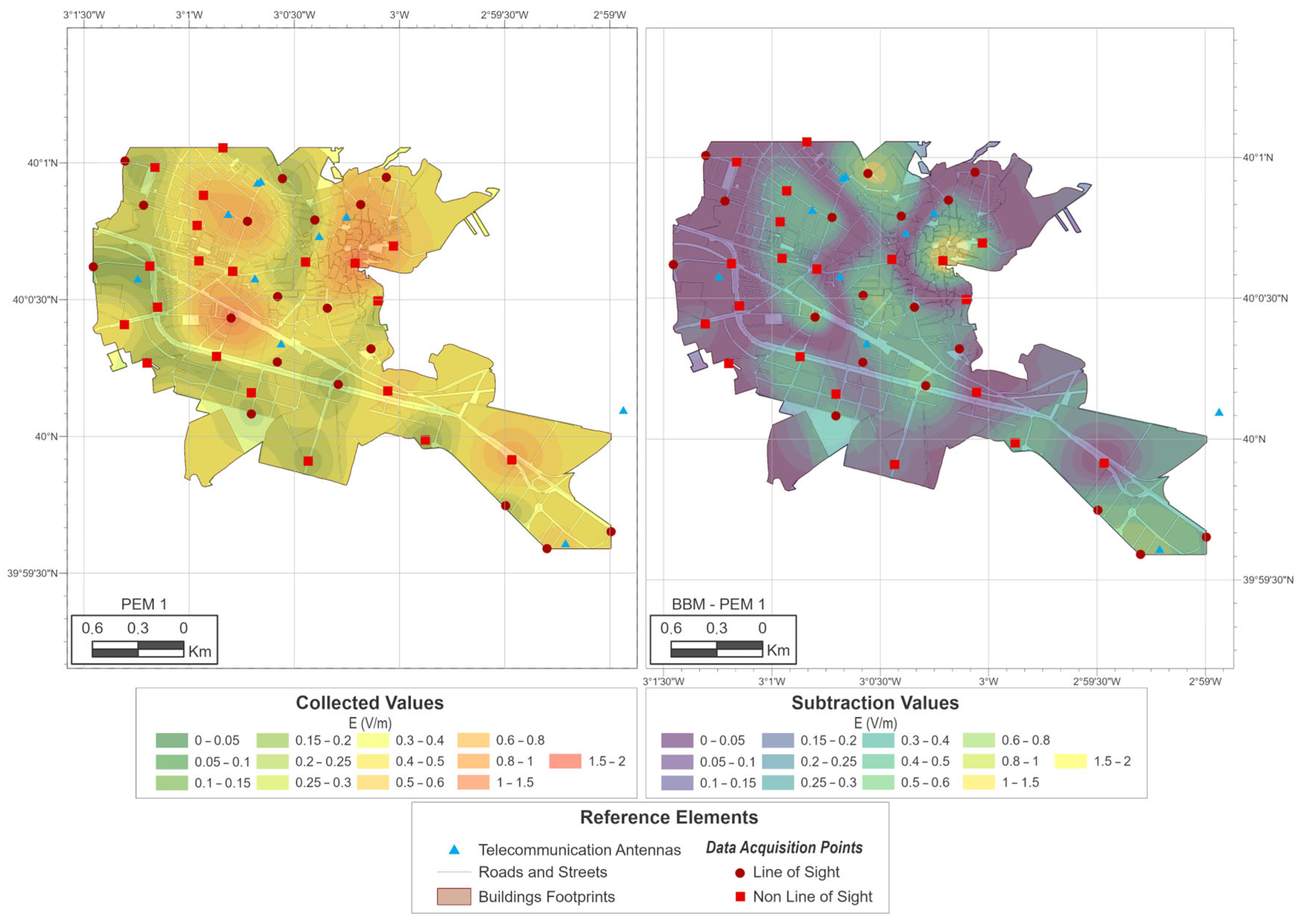
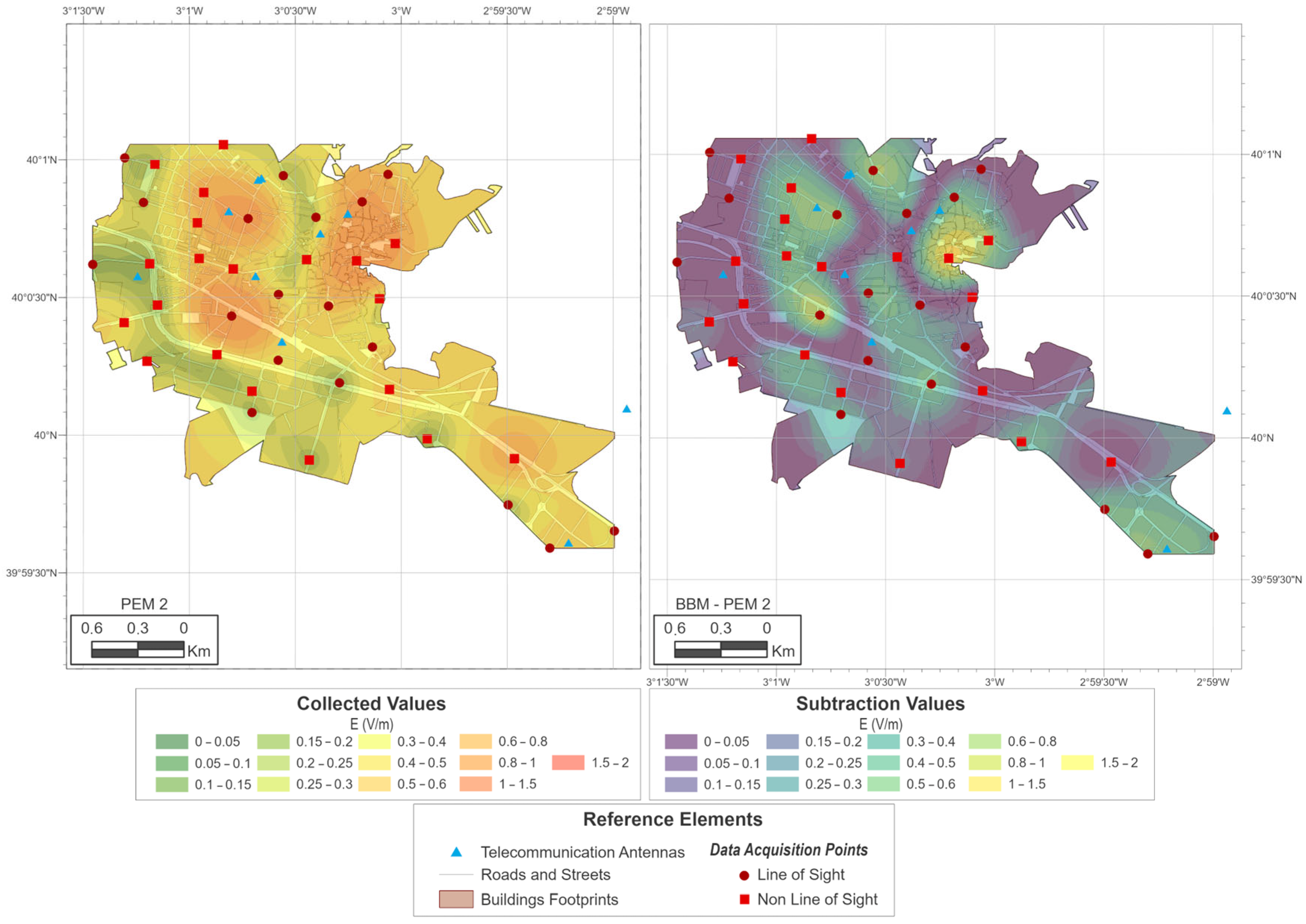
2.1. Measurement Equipment and Procedure

The set of measurements corresponds to those carried out in 38 different locations for 6 min on average, covering the urban area of Tarancón (Spain) in February 2018. A Narda BBM model EMR-300 with an 18C isotropic probe was used to carry out the measurements; it was placed at a height of 1.5 m on a non-metallic tripod EMCO 11689C. The PEM model used was the Satimo EME Spy 140. The ranges of the BBM Narda (from 100 kHz to 3 GHz) and the PEM Satimo EME Spy 140 (from 88 MHz to 5.8 GHz) do not match exactly. For this reason, the exposure meter bands above 3 GHz were discarded, and it was assumed that the contributions in the area below the FM Broadcasting Service (less than 88 MHz) can be considered negligible. During the fieldwork, and to the authors’ knowledge, no local emitters were found in the range between 100 kHz and 88 MHz that could contradict this assumption.

Static measurements were taken at specific points to compare the performance of the BBM and the PEM; the variability between BBMs and smartphones and the use of continuously moving PEMs in a closed environment were analyzed previously [9,10,11]. In this case, we used two PEM, placed on either side of the hip of the volunteer, configured to measure every 5 s. The electric field value corresponding to that location was determined from the average of the values taken during the 6 min of the measurement interval. During the 6 min measurement, the volunteer carrying the PEMs was continuously moving around the static probe placed on a tripod. There is a slight difference in height between the BBM (1.5 m) and the PEMs located at the hips (approximately 1 m). No correction for this difference is proposed in this study, as we implicitly assume that movement around the BBM can correct for the small differences in the values at the two positions. The broadband isotropic probe provides a single value of electric field, which integrates the total power measured over all bands and from every possible location, averaging the values taken across the 6 min measurement period. PEMs are usually used by travelling along the area to be measured, taking measurements at the chosen periodicity, without carrying out six-minute averages [12]. In this case, to obtain the possible equivalence for the purposes of environmental compliance and to eliminate the influence of the volunteer, a circular path around the measurement point in a range of about 3 m was proposed. The goal was to be able to produce equivalent exposure maps using BBM from a fixed point and PEM moving over a small area around that point for a measurement period of six minutes in both cases.

Note that these measurements were made prior to the revision of the ICNIRP 2020 recommendations [13] and therefore follow the previous 1998 guidelines [14]. The levels may have changed today, but the aim of this study is not to produce a map representing the current values, a task that can be undertaken in future, but to assess the possibility of making such an exposure map with a PEM instead of a BBM. The measurement points were selected following a criterion of homogeneous distribution in the urban area of the municipality. The area covered is 5.13 km² and the perimeter of the area is 10.2 km. There were 38 measurement points, so the density of points is 7.40 points/km², similar to the value discussed in other works [15] and considering typical distances between points of 0.3 Km, although some of those located in the southern area may double this value. The sites were located in open areas. For each site, the existence of direct line of sight (LOS) or not (NLOS) with any of the mobile telephony base stations (BTS) existing in the municipality was noted. In this way, the dataset is divided into 18 sites with direct line of sight to the antenna and 20 without it. The measurement points in each case and the position of the BTS are shown in Figure 1.

2.2. Statistical and Graphical Tools

The measured values, both BBM and PEM, were analyzed numerically using Statgraphics Centurión version 19.2.01 (64-bits) software [16] and IBM SPSS v.24 [17]. Using these programs, the means and variances were obtained and the fitting of the probability functions was performed.

The geographic analysis of the data was carried out using R version 4.3.2. This programming language allows for complex statistical analyses and their visualization, highlighting its capacity to process geographic data with libraries such as sp, sf, raster, gstat and automap [18,19,20,21,22]. The sp and sf libraries were used to read and process vector spatial data, while the raster library was employed for handling raster data. Ordinary kriging was carried out using the gstat package. To support this, the automap package was used to automate the fitting of the semivariogram, thereby streamlining the process. It also allows for the use of genetic algorithms from specific libraries, such as GA: Genetic Algorithm [23]. Genetic algorithms are a kind of classical optimization technique and are still used as part of more modern schemes such as the multimethod ensemble approach [24,25]. In this case, it is only a matter of finding the optimal value of two variables, so classical techniques such as genetic algorithms are suitable for the optimization process. These capabilities have led to its selection as a programming language. The interpolation technique used in this study was ordinary kriging, using the specific libraries gstat and automap [19,22]. Interpolation by kriging has been used for mapping with BBM and PEM measurements and to calculate the whole-body specific absorption rate (SAR) [15,26,27].

The gstat library was used for the development of the comparative mapping [22]. The adjustment of the semi-variogram was performed manually, using information from similar statistical analyses [3,28]. In the case of the BBM, the fit was performed with a spherical function, while the uncalibrated exposimeter (PEM) dataset showed a better fit with an exponential function. As explained in detail below, the measurements made with the PEM were corrected using a single constant for the whole range of values (PEM-1) or two different constants depending on whether there was LOS to any of the emitters at the measurement point (PEM-2). The adjustment of the semivariogram was, in both cases, conducted using a spherical function. For the integration of the spatial interpolation process with the genetic algorithm, the automatic adjustment of the automap library was used; this serves to adjust the sample to the function with the smallest error present. For this case, the following distributions were used: Spherical, Exponential, Gaussian, Spatio-Temporal Error and Matern’s Covariance [19].

The kappa variable, in the estimation of the semivariogram, allows the smoothness of the random field to be adjusted. In other words, it favors a better fit. In this case, a variable kappa value was used to test different levels of smoothness and select the one that best fitted the data. For the interpolation process, a rectangular interpolation grid of 5 × 10⁶ cells was generated. In the interpolation adjustment, the function resulting from the automatic adjustment of the semi-variogram is used. Other parameters used in the interpolations are: nmax and maxdist. The parameter nmax is used to limit the number of neighboring points that influence the estimation of a value at a specific location. The maxdist parameter, on the other hand, defines the maximum distance up to which neighboring points should be considered for interpolation. In this case, the value 10 was used for the nmax parameter and 20 for the maxdist parameter.

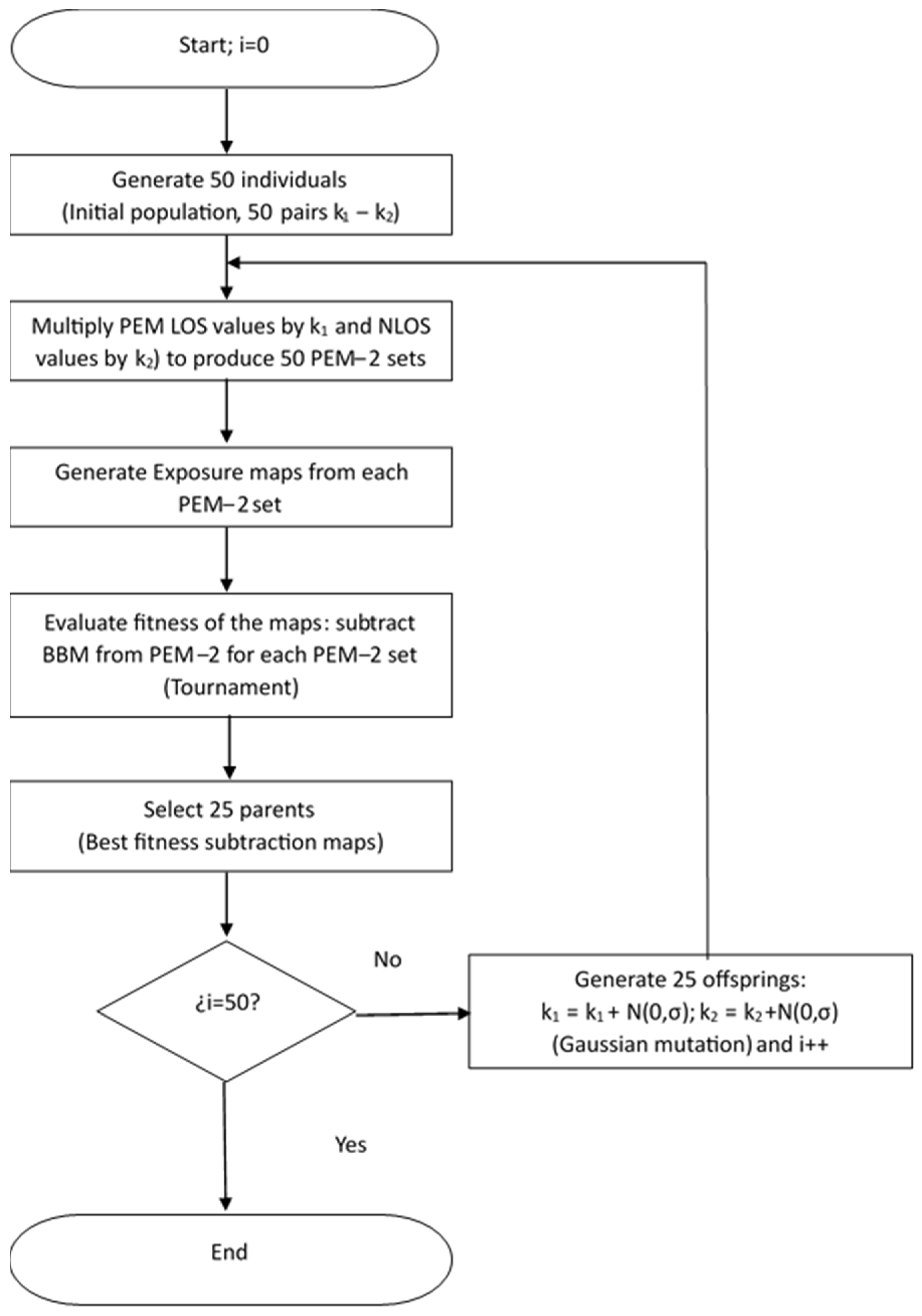
2.3. Evolutionary Programming

To establish the proportionality values of the LOS and NLOS measurement groups between PEM and BBM that best fit the generated exposure maps, a classical evolutionary algorithm has been programmed. A population of 50 individuals (pairs of k1 and k2 values representing the BBM-PEM proportionality for LOS and NLOS respectively) and a selection by tournament procedure are tested, so that the best 25 become parents of the next generation. Offspring are generated from the best 25 parents via the Gaussian mutation procedure, with no crossover (exchange of k₁ and k₂ values between individuals) allowed. The variance of the Gaussian mutation is reduced over the 50-generation run [29,30,31].

3. Results

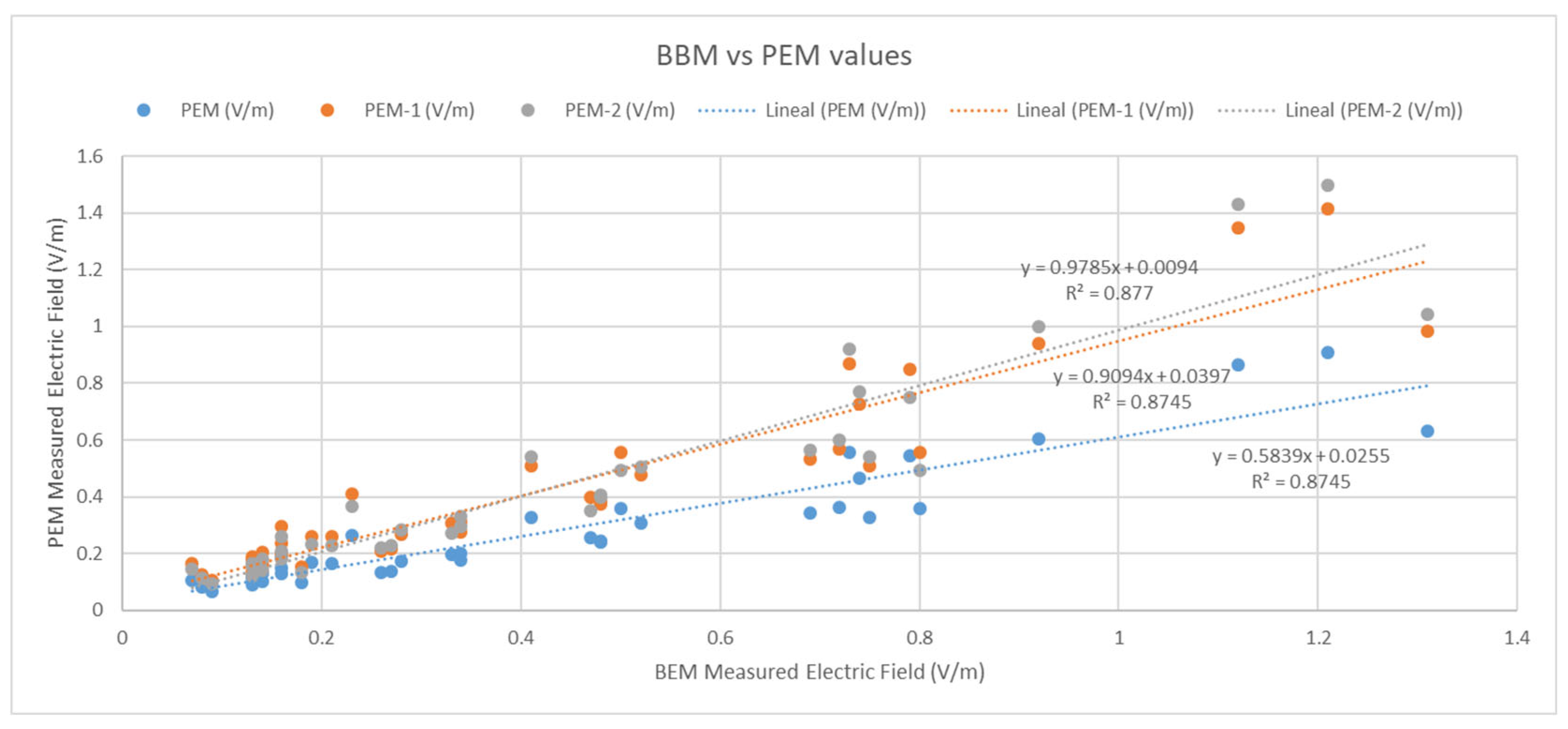
3.1. Numerical Results

The measured values at the 38 sites are shown in

Table 1. Location and values of BEM, PEM and single (PEM-1) and double (PEM-2) corrected values.

Spot #	LOS (Y/N)	Latitude	Longitude	BBM	PEM	PEM-1	PEM-2
		UTM Coord.	UTM Coord.	(V/m)	(V/m)	(V/m)	(V/m)
1	Y	39.994206	−2.983249	0.74	0.47	0.74	0.35
2	Y	39.993172	−2.98831	1.31	0.63	1.01	0.49
3	N	39.998579	−2.991105	0.79	0.54	0.87	0.75
4	N	39.999779	−2.997955	0.47	0.25	0.41	0.12
5	N	40.00277	−3.000925	0.5	0.36	0.57	0.49
6	Y	40.003162	−3.004844	0.72	0.36	0.58	0.13
7	Y	40.005329	−3.002251	0.48	0.24	0.39	0.4
8	Y	40.001367	−3.011736	0.75	0.33	0.52	0.16
9	N	40.002663	−3.011736	0.13	0.09	0.14	0.23
10	N	40.007875	−3.019171	0.13	0.11	0.18	0.14
11	N	40.004472	−3.019993	0.18	0.1	0.16	0.17
12	Y	40.010333	−3.024253	0.26	0.13	0.21	0.09
13	Y	40.007211	−3.013344	0.73	0.56	0.89	1.5
14	N	40.004878	−3.014495	0.8	0.36	0.57	0.26
15	N	40.010379	−3.019779	0.19	0.17	0.27	0.11
16	Y	40.004534	−3.009684	0.34	0.2	0.32	0.33
17	Y	40.014083	−3.020273	0.27	0.14	0.22	0.23
18	Y	40.016776	−3.021755	0.28	0.17	0.27	0.21
19	N	40.016401	−3.019377	0.16	0.19	0.3	0.18
20	N	40.017585	−3.013982	0.13	0.12	0.19	0.27
21	N	40.014692	−3.015529	0.23	0.26	0.42	0.77
22	N	40.012854	−3.01603	0.09	0.07	0.11	0.54
23	N	40.010694	−3.015893	0.08	0.08	0.13	0.6
24	N	40.01006	−3.013209	0.07	0.11	0.17	0.5
25	Y	40.013106	−3.012031	0.48	0.25	0.39	1.04
26	Y	40.015715	−3.009268	1.21	0.91	1.45	0.22
27	Y	40.013187	−3.006717	0.41	0.33	0.52	0.23
28	Y	40.015789	−3.001042	0.34	0.18	0.29	0.56
29	N	40.011602	−3.000477	0.16	0.15	0.24	0.92
30	N	40.008259	−3.001715	0.33	0.2	0.32	0.29
31	Y	40.007813	−3.00571	0.92	0.6	0.97	0.54
32	N	40.010627	−3.007441	0.21	0.17	0.27	0.28
33	Y	40.008511	−3.009652	1.12	0.87	1.39	0.41
34	Y	40.014136	−3.003077	0.69	0.34	0.55	1
35	N	39.998498	−3.00723	0.16	0.13	0.21	0.14
36	Y	39.995791	−2.991585	0.52	0.31	0.49	0.18
37	N	40.006814	−3.021794	0.14	0.1	0.17	0.37
38	N	40.010553	−3.003512	0.14	0.13	0.21	1.43
		Mean		0.44	0.28	0.44	0.44
		Median		0.34	0.2	0.31	0.31
		Standard Deviation		0.34	0.21	0.33	0.35

. At the 38 points indicated, 9982 values corresponding to 14 frequency bands were taken using the PEM. Values measured using the PEM, broken down by frequency bands, were not included to avoid excess values in the article, but they are available upon request from the authors. Instead,

Table 2. PEM Satimo EME 140 frequency bands and mean measured values.

Band	Description of Frequency Bands	Frequency (MHz)	E (V/m)
FM	Radio broadcast transmitter	88–108	0.157
TV3	Television broadcast transmitter	174–223	0.020
TETRA	Mobile communication for closed groups	380–390	0.023
TV4&5	Television broadcast transmitter	470–830	0.036
GSM + UMTS 900 (UL)	Transmission from handset to base station	880–915	0.009
GSM + UMTS 900 (DL)	Transmission from base station to handset	925–960	0.163
GSM 1800 (UL)	Transmission from handset to base station	1710–1785	0.010
GSM 1800 (DL)	Transmission from base station to handset	1805–1880	0.036
DECT	Digital enhanced cordless telecommunications	1880–1900	0.050
UMTS 2100 (UL)	Transmission from handset to base station	1920–1980	0.005
UMTS 2100 (DL)	Transmission from base station to handset	2110–2170	0.079
Wi-Fi 2G	Wireless local area network	2400–2500	0.021
WiMAX	Worldwide interoperability for microwave access	3400–3800	0.020
Wi-Fi 5G	Wireless local area network	5150–5850	0.049

shows the ranges of the PEM frequency bands and the average of the EMF-measured values in each band. The number of decimal places offered by the PEM is higher, since the accuracy of the BBM is two digits; however, in order to improve the presentation, a number of decimal places equal to 3 is considered in Table 2. In the rest of the EMF values, where both types of measurements are compared, 2 decimal places are used to facilitate the reading. In Table 1, first, the site number (SPOT #) and the LOS-NLOS conditions are given. The next two columns correspond to the UTM coordinates of the measurement point. Then, there are the direct measurements made with the BBM EMR-300 and those made with the pair of Satimo 140 PEMs. Finally, the measurements are corrected using a single correction factor (PEM-1) as described by Bolte [32] and using a double correction factor (PEM-2) according to the LOS-NLOS condition. The values of the PEM-1 and PEM-2 columns were obtained by equating the mean value of the BBM and PEM column values in the single or dual correction cases. For the sake of comparison, measured and corrected values are given using two decimals. In the PEM-1 case, the ratio between both measurement sets is 1.557. In the PEM-2 case, the ratio between LOS values is 1.651 and that between NLOS values is 1.380. Further details of these corrections are given in the discussion section.

When comparing the four measurement sets (Figure 2), it is observed that measurements taken with the PEM (blue line) tend to underestimate, especially the higher values (generally, those measured in LOS conditions). The ideal slope of the straight line for the corrected measurements should be 1, and this value is practically reached with the proposed double correction (PEM-2, grey line) instead of the single correction (PEM-1, blue line) with similar values of the R² coefficient.

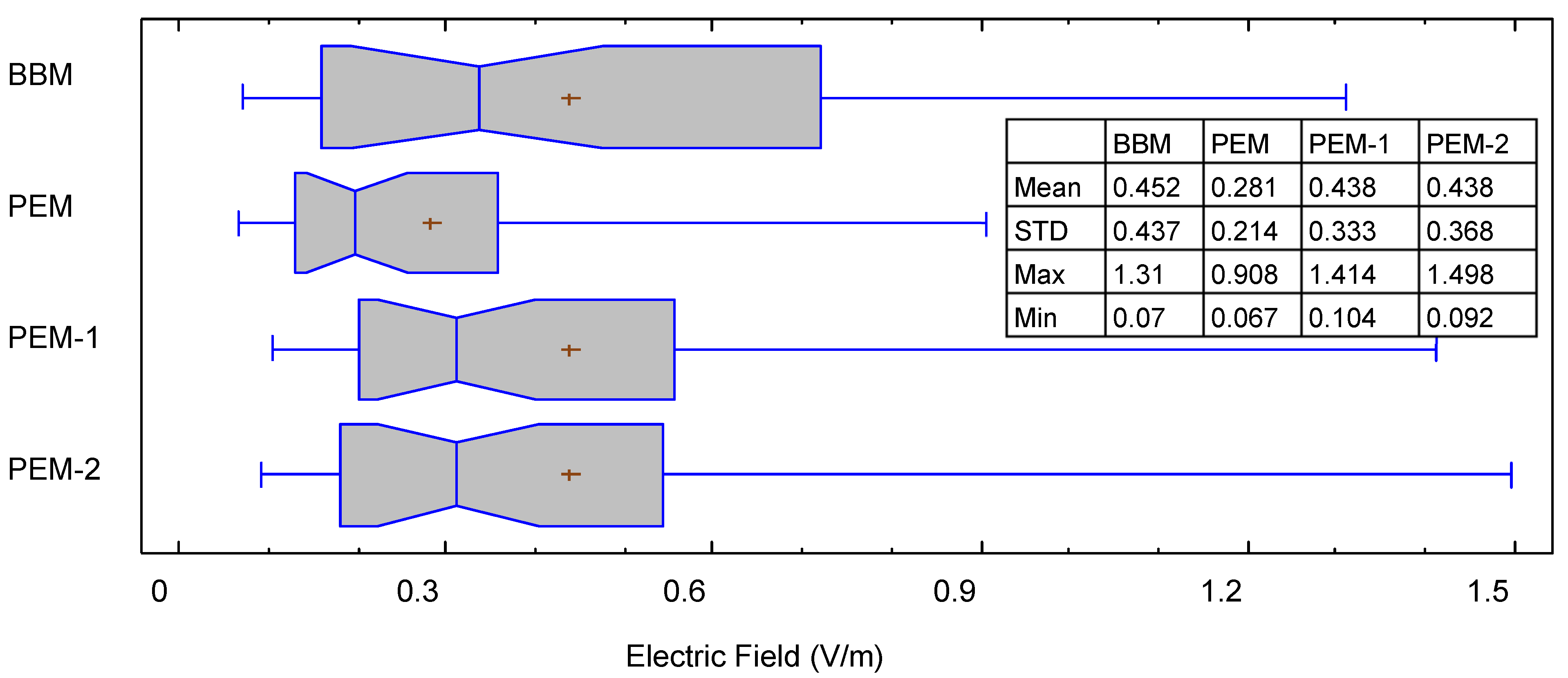
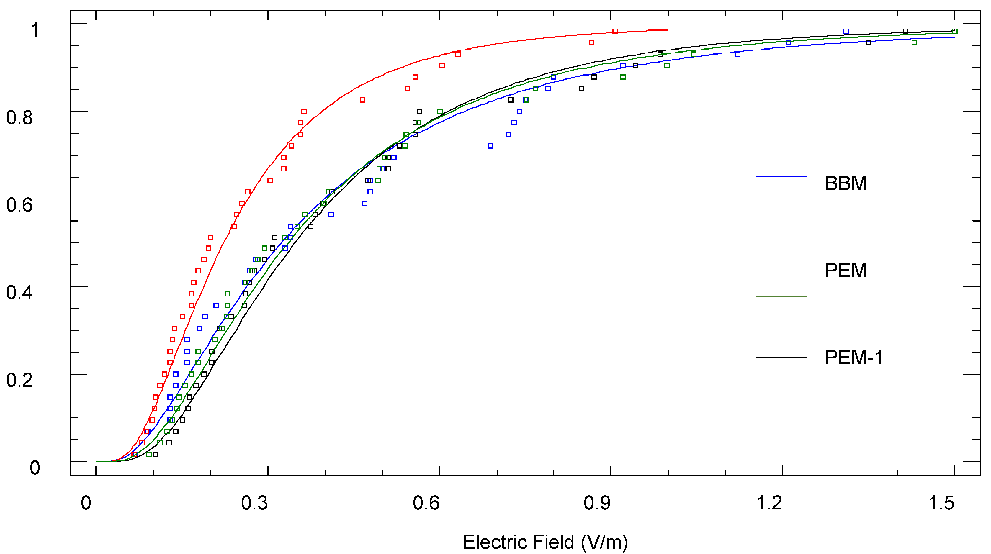
3.2. Statistical and Graphical Results

The main statistical values of the measurements are shown in Figure 3. Although the mean values are similar, there are differences between the ranges of measurements and, to a lesser extent, between the standard deviations of the sample. The mean BBM measurement value was 0.438 V/m (IC95%: 0.328–0.548) and we determined a value of 0.281 V/m for the PEM measurements (IC95%: 0.213–0.350). The BBM and PEM measurements showed a rho Spearman correlation of 0.948 ** (p < 0.01). Taking this value into account, the mean PEM exposure value should be 0.438 V/m (IC95%: 0.340–0.561). We also performed a U–Mann-Whitney test (BBM and corrected PEM measurements) that found no statistically significant differences (p > 0.05).

Figure 4 shows the statistical fit to the lognormal distribution as described by [3]. The proposed double correction (green) achieves a better statistical fit of the BBM values (blue).

To check the validity of these adjustments in the realization of exposure maps, the sets of measurements were plotted on cartographic maps using the kriging method using R software [33]. First, the exposure map corresponding to the Narda EMR 300 BBM measurement was obtained (Figure 5). The maps obtained for the PEM, PEM-1 and PEM-2 sets and the differences with respect to the map of the BBM points are shown below (Figure 6, Figure 7 and Figure 8).

As shown in Figure 5, the highest exposure values are concentrated near the BTS. If this map is compared with the PEM maps, some differences in the interpolation can be seen that were not revealed by the previous analyses. First, the map obtained using the direct PEM measurements (Figure 6) is able to determine the areas with the highest level of exposure, but not the spatial variation; it therefore offers greater gradients of variation towards the areas with lower levels. The corrections made to the personal exposure meter measurements correct this defect to some extent but still offer differences with respect to the original map. In the PEM-1 case (Figure 7), even higher maximum values can be seen. In this sense, the simple correction of the dataset can lead, after the kriging interpolation process, to an overestimation of the exposure reflected in the map. In the PEM-2 case (Figure 8), the areas with the highest level of error are minimized. There are still some areas (SE of the map) where errors have not been corrected. It is possible that this is due to a defect in the planning of the sampling, which does not correctly establish the perimeter of the area under study.

3.3. Genetic Algorithm Adjustment

The differences shown in the maps above suggest that the dataset adjustments after mean correction—particularly in the PEM-1 case—are not well suited for producing an exposure map. For this reason, we analyzed the possibility of finding an adjustment that minimizes the differences between the map obtained by means of the BBM and the corrected PEM and not between the mean values of both sets. The differentiation between LOS and NLOS measurements was maintained in order to increase the degree of freedom of the algorithm. Figure 9 shows the flowchart followed. Each individual in the population consists of two values (k₁ and k₂), which are the proportionality constants between the LOS and NLOS measurement subsets, respectively. First, the exposure map corresponding to the BBM measurements is obtained. This map is identical to the one in Figure 5. An initial population of 50 individuals is generated. Their values of k₁ and k₂ are obtained as 1 + N (0, 1), the latter being a normal distribution of mean 0 and standard deviation 1. With these values, an automatic estimation of the semi-variogram is performed with the autofitVariogram function of the R AutoMap library. Based on this analysis, it is possible to determine the relationship between the distance of the samples and the difference in the acquired measurements. Once the semivariogram has been estimated and adjusted, the krige function of the gstat library is used to perform the interpolation with kriging, resulting in a raster layer with the continuous distribution of the variable. This layer is then clipped to the study area. Once all the solutions necessary for the analysis have been extracted, they are normalized in values from 0 to 255. Subsequently, to determine the differences, the Structural Similarity Index of the layers obtained is determined by taking the layer generated with the BBM data as the good image and subtracting those obtained from the genetic solutions. Therefore, the exposure maps of each individual are generated and then subtracted from the BBM map. The sum of the absolute value of the difference at each point on the surface corresponds to the fitness function (absolute value of the difference between both maps). The 25 best values correspond to the individuals that will be parents of the next generation. The offspring are obtained by adding to each parent a random value of mean 0 and decreasing variance (σ) over the following generations. The process is repeated until 50 generations have been completed.

Evolutionary algorithms are characterized by obtaining a different solution on each run. Successive runs yield a range of sub-optimal solutions of the constants k₁ and k₂. For this reason, the algorithm shown in Figure 9 was run five times, obtaining the best values shown in

Table 3. Best pairs of k₁ and k₂ values obtained in each iteration.

Iteration #	k1	k2
1	1.7011	1.3241
2	1.4805	1.2490
3	1.5799	1.3338
4	1.4853	1.2619
5	1.6643	1.4062

.

The final values of k₁ and k₂ are in the ranges 1.7011–1.4853 and 1.4062–1.2490, respectively. These ranges are consistent with the values obtained from the relationship found in Section 3.1 (1.651 and 1.380, respectively). Using the pair of values corresponding to the first iteration, the exposure map and the difference map shown in Figure 10 were produced. This solution is indicated as PEM-G, since a double correction is made, and the values of which were obtained by means of a genetic algorithm. Although differences are observed in the areas of maximum exposure, the values are lower than in the previous cases. The discussion section contains an analysis of the limitations of this method, which lead to the persistence of differences.

4. Discussion

In this study, we compared radiofrequency electromagnetic field (RF-EMF) exposure measurements obtained using a broadband meter (BBM) and a personal exposimeter (PEM). The primary objective was to evaluate the necessary adjustments for making personal exposimeter measurements comparable to those from broadband meters when developing exposure maps. We analyzed the data collected and studied two correction approaches: a single correction factor and a double correction factor, depending on the existence of direct line of sight (LOS) to base stations. Additionally, we implemented a genetic algorithm to enhance the accuracy of exposure maps generated from PEM measurements and obtaining a range of values of the tested proportionality factors.

Measurements made with the PEM tend to underestimate the value corresponding to the measurement site. This is due to the shielding of the body over the meter [34], which implies a lower final value. In the work of Bolte et al., a single correction factor is proposed over the whole set of measurements. Due to this shielding of the body, especially in the direct vision measurements, we proposed different correction depending on whether the measurement is made under LOS conditions to the BTS. If so, there is a predominant contribution in the received electric field due to this component, and its possible shielding significantly reduces the value measured by the PEM.

When there is NLOS, the measured field value is due to several secondary contributions coming from the multipath of the signal, so that the possible shielding of some of them has less influence on the measured value. According to this hypothesis, we calculated correction factors for both cases. Considering a single factor gives a weighting factor for the measures of 1.557. This factor is consistent with that obtained by Bolte et al. (1.06 to 1.57) [32]. On the other hand, if the dataset is divided, a correction factor of 1.650 is obtained for LOS measurements and 1.380 for the rest.

This second correction (PEM-2) achieves a better fit of the statistical values of the dataset between the BBM and the PEM. However, when it comes to representing these values on an exposure map, significant differences are observed both in the maximum exposure values obtained on the map and in their spatial variations when moving away from them.

These types of corrections are based on equalizing the mean values of datasets or subsets of data. Since the final objective is the representation of exposure maps, an optimization was tested using a genetic algorithm that tries to minimize the differences between the exposure maps to be generated. The results obtained indicate that the differences between the proportionality constants for both subsets of data are more extreme than in the case of the calculation of the mean, even exceeding the limits determined by Bolte for a single correction.

The largest differences in the exposure maps are obtained around the maxima, especially in the cases of the Bolte correction (PEM-1). For this reason, a different strategy was tested, which focuses on matching the spatial representations of exposure rather than just equalizing the average values of the data. A genetic algorithm was applied to optimize the proportionality constants between the LOS and NLOS measurement subsets. The goal was to minimize the differences between the exposure maps generated with BBM and the corrected PEM measurements. This approach allowed for more precise corrections, particularly in urban environments where the exposure can vary significantly depending on the presence of direct line of sight to base stations. By adjusting these factors through an evolutionary process, we aimed to produce exposure maps that were more consistent and reflective of the actual RF-EMF distribution.

Results from the genetic algorithm show a promising improvement in the spatial accuracy of the exposure maps. The corrected PEM measurements, using the genetically optimized factors, provided exposure distributions that more closely mirrored those obtained with BBM. While some local variations still exist, especially in areas with complex urban architecture, the overall accuracy of the PEM-generated maps significantly increased. This approach demonstrates the potential of using PEM devices with proper calibration and correction to produce reliable and cost-effective RF-EMF exposure maps.

Limitations

Despite the promising results obtained in this study, several limitations need to be acknowledged. First, a relatively limited number of measurement points were used to compare PEM and BBM measurements, which may affect the generalizability of the results to other urban areas or more complex environments. Future research should consider increasing the number of measurement points and conducting studies in diverse locations to validate the applicability of the proposed correction factors.

Second, the body shielding effect on the PEM remains a challenging factor to fully model. While differentiated corrections for LOS and NLOS conditions were applied, other environmental factors, such as the presence of architectural structures or unidentified interference sources, may also affect the measurements.

Limitations concerning the geographical interpolation of the values themselves must also be considered. The kriging technique is characterized by obtaining an interpolation surface that does not contain the measured values; rather, it searches for trends in them. For this reason, the correction of the sets of points does not guarantee identical results in the realization of the maps.

Some of the weaknesses in the set of measurements used should also be highlighted; these may lead to problems in the generation of interpolation maps. Considering the location of the measurement points, the southern and eastern areas of the municipality do not have measurement points on the perimeter, which can lead to errors at the extremes of the interpolation surface; this will consequently lead to incorrect fitness adjustment values. Similarly, in the base stations located further east of the municipality, a greater number of measurements should have been made.

In addition to the above issues, we must also consider a possible difference between the measurements made with both devices. In the proportional correction of both measurement subsets, it is implicitly assumed that the sensitivity and linearity of both instruments over their entire measurement range are identical. Although this assumption can be taken as true for properly calibrated equipment, non-linear solutions that optimize the kriging results could be tested.

Finally, although the use of the genetic algorithm improved the accuracy of the exposure maps, this technique is computationally intensive and may not be easily applicable in all cases, especially in studies requiring real-time results. The presented methodology could benefit from the incorporation of faster optimization techniques or the integration of predictive models to reduce the need for extensive corrections.

5. Conclusions

We conclude that exposure assessments based on spot measurements can serve as a practical proxy to evaluate personal RF-EMF exposure, whether using a static probe or a portable PEM. The developed methodology offers a reliable and efficient approach to characterizing personal exposure levels, enabling continuous monitoring and the detection of potential changes over time. The result of the different proportionality factors obtained is shown in

Table 4. Proportionality ratios between the different sets.

	PEM	PEM-1	PEM-2	PEM-G (Range)
k1	1	1.557	1.650	1.7011–1.4853
k2	1	1.557	1.380	1.4062–1.2490

.

The application of correction factors, particularly the differentiation between LOS and NLOS conditions, significantly improves the accuracy of PEM measurements, bringing them closer to those obtained with BBMs. This highlights the importance of accounting for the line of sight to antennas when estimating exposure levels, as direct exposure to base stations considerably affects measurement accuracy due to body shielding effects. By applying appropriate correction factors, the inherent limitations of PEMs, such as underestimating exposure levels in LOS conditions, can be mitigated.

Moreover, using genetic algorithms to optimize these corrections further enhances the precision of the exposure maps, demonstrating that this method can be a valuable tool in urban RF-EMF monitoring. The ability to generate accurate spatial exposure distributions through PEMs makes this methodology more accessible and cost effective, especially in large-scale studies where deploying multiple BBMs might not be feasible.

Nevertheless, further validation is needed in various environments to refine the correction models and ensure broader applicability. Future studies should focus on refining these algorithms and exploring other factors that could influence exposure, such as linearity, urban infrastructure, and signal interference. Despite these challenges, the methodology developed in this study represents a significant advancement in RF-EMF exposure assessment, offering a flexible and scalable approach to creating consistent EMF exposure maps using PEMs.

References

1. Bosch-Capblanch, X.; Esu, E.; Dongus, S.; Oringanje, C.M.; Jalilian, H.; Eyers, J.; Oftedal, G.; Meremikwu, M.; Röösli, M. The effects of radiofrequency electromagnetic fields exposure on human self-reported symptoms: A systematic review of human experimental studies. Environ. Int. 2024, 187, 108612. [Google Scholar] [CrossRef] [PubMed]
2. Ramirez-Vazquez, R.; Escobar, I.; Vandenbosch, G.A.E.; Vargas, F.; Caceres-Monllor, D.A.; Arribas, E. Measurement studies of personal exposure to radiofrequency electromagnetic fields: A systematic review. Envrion. Res. 2023, 218, 114979. [Google Scholar] [CrossRef] [PubMed]
3. Sánchez-Montero, R.; Alén-Cordero, C.; López-Espí, P.L.; Rigelsford, J.M.; Aguilera-Benavente, F.; Alpuente-Hermosilla, J. Long term variations measurement of electromagnetic field exposures in Alcalá de Henares (Spain). Sci. Total Environ. 2017, 598, 657–668. [Google Scholar] [CrossRef]
4. Sagar, S.; Struchen, B.; Finta, V.; Eeftens, M.; Röösli, M. Use of portable exposimeters to monitor radiofrequency electromagnetic field exposure in the everyday environment. Environ. Res. 2016, 150, 289–298. [Google Scholar] [CrossRef] [PubMed]
5. Frei, P.; Mohler, E.; Bürgi, A.; Fröhlich, J.; Neubauer, G.; Braun-Fahrländer, C.; Röösli, M.; QUALIFEX Team. Classification of personal exposure to radio frequency electromagnetic fields (RF-EMF) for epidemiological research: Evaluation of different exposure assessment methods. Environ. Int. 2010, 36, 714–720. [Google Scholar] [CrossRef]
6. Chikha, W.B.; Zhang, Y.; Liu, J.; Wang, S.; Sandeep, S.; Guxens, M.; Veludo, A.F.; Röösli, M.; Joseph, W.; Wiart, J. Assessment of Radio Frequency Electromagnetic Field Exposure Induced by Base Stations in Several Micro-Environments in France. IEEE Access 2024, 12, 21610–21620. [Google Scholar] [CrossRef]
7. Sagar, S.; Dongus, S.; Schoeni, A.; Roser, K.; Eeftens, M.; Struchen, B.; Foerster, M.; Meier, N.; Adem, S.; Röösli, M. Radiofrequency electromagnetic field exposure in everyday microenvironments in Europe: A systematic literature review. J. Expo. Sci. Envrion. Epidemiol. 2018, 28, 147–160. [Google Scholar] [CrossRef]
8. IEEE Std C95.3-2002; Recommended Practice for Measurements and Computations of Radio Frequency Electromagnetic Fields with Respect to Human Exposure to Such Fields, 100 kHz-300 GHz; IEEE Std C95.3-2002 (Revision of IEEE Std C95.3-1991). IEEE: Piscataway, NJ, USA, 2002; p. 126. [CrossRef]
9. Ramirez-Vazquez, R.; Gonzalez-Rubio, J.; Arribas, E.; Najera, A. Personal RF-EMF exposure from mobile phone base stations during temporary events. Environ. Res. 2019, 175, 266–273. [Google Scholar] [CrossRef]
10. López-Espí, P.L.; Sánchez-Montero, R.; Guillén-Pina, J.; Castro-Sanz, R.; Chocano-del-Cerro, R.; Martínez-Rojas, J.A. Smartphone-Based Methodology Applied to Electromagnetic Field Exposure Assessment. Sensors 2024, 24, 3561. [Google Scholar] [CrossRef]
11. Sandoval-Diez, N.; Belácková, L.; Veludo, A.F.; Jalilian, H.; Guida, F.; Deltour, I.; Thielens, A.; Zahner, M.; Fröhlich, J.; Huss, A.; et al. Determining the relationship between mobile phone network signal strength and radiofrequency electromagnetic field exposure: Protocol and pilot study to derive conversion functions. Open Res. Eur. 2024, 4, 206. [Google Scholar] [CrossRef]
12. Paniagua-Sánchez, J.M.; García-Cobos, F.J.; Rufo-Pérez, M.; Jiménez-Barco, A. Large-area mobile measurement of outdoor exposure to radio frequencies. Sci. Total Environ. 2023, 877, 162852. [Google Scholar] [CrossRef] [PubMed]
13. International Commission on Non-Ionizing Radiation Protection (ICNIRP). Guidelines for Limiting Exposure to Electromagnetic Fields (100 kHz to 300 GHz). Health Phys. 2020, 118, 483–524. Available online: https://www.icnirp.org/cms/upload/publications/ICNIRPrfgdl2020.pdf (accessed on 25 June 2025). [CrossRef]
14. International Commission on Non-Ionizing Radiation Protection (ICNIRP). Guidelines for limiting exposure to time-varying electric, magnetic, and electromagnetic fields (up to 300 GHz). Health Phys. 1998, 74, 494–522. [Google Scholar]
15. López-Espí, P.L.; Sánchez-Montero, R.; Guillén-Pina, J.; Chocano-del-Cerro, R.; Rojas, J.A.M. Optimal design of electromagnetic field exposure maps in large areas. Environ. Impact Assess. Rev. 2024, 106, 107525. [Google Scholar] [CrossRef]
16. Statgraphics Technologies Inc. Statgraphics Centurion 19. Available online: https://www.statgraphics.com/download19 (accessed on 27 September 2024).
17. IBM Corporation. IBM SPSS Statistics v. 24. 2017. Available online: https://www.ibm.com/es-es/products/spss-statistics (accessed on 27 September 2024).
18. Bivand, R.S.; Pebesma, E.; Gómez-Rubio, V. Applied Spatial Data Analysis with R; Springer: New York, NY, USA, 2013. [Google Scholar] [CrossRef]
19. Hiemstra, P. Automap: Automatic Interpolation Package. 2023. Available online: https://CRAN.R-project.org/package=automap (accessed on 18 August 2024).
20. Hijmans, R.J. Raster: Geographic Data Analysis and Modeling. 2023. Available online: https://CRAN.R-project.org/package=raster (accessed on 30 September 2024).
21. Pebesma, E. Simple Features for R: Standardized Support for Spatial Vector Data. R J. 2018, 10, 439. [Google Scholar] [CrossRef]
22. Pebesma, E. Gstat: Spatial and Spatio-Temporal Geostatistical Modelling, Prediction, and Simulation. 2023. Available online: https://CRAN.R-project.org/package=gstat (accessed on 30 September 2024).
23. Scrucca, L. GA: A Package for Genetic Algorithms in R. J. Stat. Softw. 2013, 53, 1–37. [Google Scholar] [CrossRef]
24. Salcedo-Sanz, S.; Del Ser, J.; Landa-Torres, I.; Gil-López, S.; Portilla-Figueras, J.A. The Coral Reefs Optimization Algorithm: A Novel Metaheuristic for Efficiently Solving Optimization Problems. Sci. World J. 2014, 2014, 1–15. [Google Scholar] [CrossRef]
25. Wu, G.; Mallipeddi, R.; Suganthan, P.N. Ensemble strategies for population-based optimization algorithms–A survey. Swarm Evol. Comput. 2019, 44, 695–711. [Google Scholar] [CrossRef]
26. Rufo-Pérez, M.; Antolín-Salazar, A.; Paniagua-Sánchez, J.M.; Jiménez-Barco, A.; Rodríguez-Hernández, F.J. Spatial and Temporal Mapping of RF Exposure in an Urban Core Using Exposimeter and GIS. Sensors 2025, 25, 1301. [Google Scholar] [CrossRef]
27. Jawad, O.; Lautru, D.; Benlarbi-Delai, A.; Dricot, J.-M.; Doncker, P. Study of Human Exposure Using Kriging Method. Prog. Electromagn. Res. B 2014, 61, 241–252. [Google Scholar] [CrossRef]
28. Guillén-Pina, J.; Pérez-Aracil, J.; Chocano-del-Cerro, R.; Sánchez-Montero, R.; López-Espí, P.L.; Salcedo-Sanz, S. Efficient design of electromagnetic field exposure maps with multi-method evolutionary ensembles. Environ. Res. 2025, 278, 121636. [Google Scholar] [CrossRef] [PubMed]
29. Goldberg, D.E. Genetic Algorithms in Search, Optimization, and Machine Learning. In Addison Wesley Series in Artificial Intelligence; Addison-Wesley: Boston, MA, USA, 1989. [Google Scholar]
30. Schwefel, H.-P. Numerical Optimization of Computer Models; John Wiley & Sons, Inc.: Hoboken, NJ, USA, 1981. [Google Scholar]
31. Yao, X.; Liu, Y.; Lin, G. Evolutionary programming made faster. IEEE Trans. Evol. Comput. 1999, 3, 82–102. [Google Scholar] [CrossRef]
32. Bolte, J.F.B.; van der Zande, G.; Kamer, J. Calibration and uncertainties in personal exposure measurements of radiofrequency electromagnetic fields. Bioelectromagnetics 2011, 32, 652–663. [Google Scholar] [CrossRef] [PubMed]
33. R Core Team. R: A Language and Environment for Statistical Computing. 2023. Available online: https://www.R-project.org/ (accessed on 18 August 2024).
34. Bolte, J.F.B. Lessons Learnt on Biases and Uncertainties in Personal Exposure Measurement Surveys of Radiofrequency Electromagnetic Fields with Exposimeters; Elsevier Ltd.: Amsterdam, The Netherlands, 2016. [Google Scholar] [CrossRef]
Figure 1. Distribution of measuring locations and BTS.
Applsci 15 07471 g001
Figure 2. Ratio of measured BBM values to PEM, PEM-1, and PEM-2 values.
Applsci 15 07471 g002
Figure 3. Mean value, standard deviation, and measured ranges of the different datasets.
Applsci 15 07471 g003
Figure 4. Cumulative probability and lognormal distribution fitting for the different datasets.
Applsci 15 07471 g004
Figure 5. Narda BBM exposure map.
Applsci 15 07471 g005
Figure 6. Satimo PEM and differences in the PEM vs. BBM exposure maps.
Applsci 15 07471 g006
Figure 7. PEM-1 and difference between PEM-1 and BBM exposure maps.
Applsci 15 07471 g007
Figure 8. PEM-2 and differences in the PEM-2 vs. BBM exposure maps.
Applsci 15 07471 g008
Figure 9. Flowchart of the evolutionary algorithm optimization.
Applsci 15 07471 g009
Figure 10. PEM-G and difference between the PEM-G and BBM exposure maps.
Applsci 15 07471 g010