Abstract
Understanding tortuosity is essential for accurately modeling fluid flow in complex porous media, particularly in the sub-surface reservoir rock; therefore, tortuosity estimation was evaluated using three approaches: Streamline streamline simulations via the Lattice Boltzmann Method (LBM), geometric pathfinding using Dijkstra’s algorithm, and empirical modeling based on pore-structure parameters. The analysis encompassed 1963 micro-Computed Tomography (micro-CT) images of Brazilian pre-salt carbonate and sandstone samples, with the effective porosity extracted from LBM velocity fields, isolating flow-contributing pores, establishing streamline tortuosity as the reference standard. Sandstones exhibited relatively narrow tortuosity ranges (Dijkstra: 1.29–1.75; Streamline: 1.18–2.61; Empirical: 1.18–4.42), whereas carbonates display greater heterogeneity (Dijkstra: 1.00–3.18; Streamline: 1.00–3.68; Empirical: 1.59–4.93). Model performance assessed using the corrected Akaike Information Criterion (AICc) revealed that the best agreement with the data was achieved by the semi-empirical model incorporating coordination number and minimum throat length (AICc = −113.11), followed by the Dijkstra-based geometrical approach (−99.74) and the empirical porosity-based model (202.23). There was a nonlinear inverse correlation between tortuosity and effective porosity across lithologies. This comprehensive comparison underscores the importance of incorporating multiple pore-scale parameters for robust tortuosity prediction, improving the understanding of flow behavior in heterogeneous reservoir rocks.
1. Introduction
Understanding the characteristics of fluid flow within porous media is crucial for predicting transport phenomena in various subsurface applications, such as hydrocarbon recovery, groundwater hydrology, and underground geophysics. One of the key parameters governing flow efficiency is tortuosity, an intrinsic property that measures the extent to which fluid flow paths deviate from a straight line through the pore structure [1,2,3]. In the context of rocks as petroleum reservoirs, tortuosity reflects the geometric complexity of the pores and the ability of the pore network to facilitate fluid flow. High tortuosity generally indicates convoluted and resistive flow paths, thereby hindering fluid transport efficiency through reduced flow velocity and altered pressure distribution according to the fundamental principles of porous flow, such as Darcy’s law. Tortuosity is inversely related to porosity and permeability since more complex flow paths tend to reduce flow space and the medium’s capacity to transmit fluids [4,5,6].
Rock types such as sandstone and carbonate have significant hydrocarbon potential, with the relatively uniform pore system in sandstone dominated by intergranular pores formed during deposition and early diagenesis [7,8,9]. Consequently, sandstone exhibits relatively homogeneous petrophysical properties and a more predictable relationship between porosity, permeability, and tortuosity compared to carbonate rocks. However, diagenetic processes such as cementation, local dissolution, and structural deformation can significantly alter the pore system, affecting connectivity and tortuosity [10,11].
In contrast, carbonate rocks, especially Brazilian pre-salt carbonate, also possess very high hydrocarbon potential but with more complex structures [12,13] due to long geological evolution and intensive diagenetic processes [14,15]. Unlike the relatively uniform pore system of sandstone, pre-salt carbonate formed in a lacustrine (ancient lake) environment beneath salt layers undergoes a series of processes such as dolomitization, selective dissolution, recrystallization, with the overburden pressure of thick salt layers causing thermal and tectonic influences [16,17,18]. Consequently, the pore system is highly heterogeneous, consisting of a combination of intergranular pores, moldic pores, vuggy pores, and micro- to macro-fractures. The pores vary in shape and size, as well as connectivity and directional orientation, creating a highly anisotropic medium [19]. The resulting fluid flow paths are not homogeneous or isotropic, thus posing significant challenges in representing and accurately calculating actual flow paths within the rock. Therefore, a multidisciplinary approach is necessary to quantify tortuosity while describing its relationship with other physical parameters such as throat radius, porosity, and permeability [6].
Tortuosity is classified into several types, including geometric, hydraulic, diffusive, and electrical tortuosity [20]. This study focuses on geometric tortuosity (Dijkstra) and flow tortuosity (Streamline), comparing both with tortuosity values obtained from mathematical formulations. Typically, Dijkstra is calculated using shortest-path algorithms applied to digital representations of the pore structure. These algorithms have proven effective in modeling pore networks in both two-dimensional (2D) and three-dimensional (3D) rock structures [21]. Since flow tortuosity represents the actual path traveled by the fluid through the porous medium, it is derived from the velocity field obtained via numerical flow simulations such as the Lattice Boltzmann Method (LBM), which is widely employed due to its advantages in handling complex boundaries and realistic porous media geometries [22,23,24,25]. Flow tortuosity is calculated from the streamline visualizations derived from the velocity field and is the ratio between the total length of the traced streamline representing the actual fluid trajectory through the pore space and the straight line distance between the inlet and outlet boundaries of the sample domain [26,27,28].
Tortuosity can also be estimated using empirical or semi-theoretical equations involving petrophysical parameters such as effective porosity, coordination number, and throat length derived from segmentation and digital characterization of the pore structure [29]. Several classical models remain in use due to their ease of implementation and ability to provide reasonably representative initial estimates. However, their accuracy is highly influenced by the pore morphology complexity and the validity of the homogeneity assumptions inherent in these models [30,31,32].
Table 1 summarizes the approaches used by various authors to evaluate tortuosity. Matyka et al. [28] employed 2D synthetic data to evaluate flow tortuosity and compared it with several empirical models. In comparison, Panini et al. [2] estimated geometric tortuosity from 3D images of carbonate and sandstone rocks and compared these values with those obtained from various empirical models. Meanwhile, Nurcahya et al. [26] calculated multiple petrophysical parameters, including tortuosity, from 2D images using the A* algorithm. Subsequently, the authors extended this approach to 3D data, focusing on streamline-based tortuosity estimation and analysis of other relevant physical parameters for porous media characterization [33].

Table 1.
Comparison of tortuosity studies.
A relevant precedent can also be found in the work by Bini et al. [34], which proposed a Lagrangian particle-based finite element model to simulate Brownian motion within trabecular bone structures reconstructed from micro-CT imaging. Their study highlights the value of combining high-resolution microstructural data with numerical simulation to investigate transport phenomena in complex porous media. This approach shares conceptual similarities with the present work, which employs micro-CT-based reconstructions and numerical analysis to evaluate tortuosity in geological samples. The alignment between these studies underscores the broader applicability of image-based modeling frameworks across disciplines involving porous structures.
While previous studies have investigated tortuosity using various methods and rock types, none have comprehensively combined geometric tortuosity, flow tortuosity, and empirical model estimations across a large 3D dataset of sandstone and carbonate rocks. This study integrated numerical modeling, digital image analysis, and empirical model evaluation to provide new insights into the complexity of pore structures and fluid flow in porous media, particularly within the highly heterogeneous pre-salt carbonate formations. The findings are expected to support improved data-driven decision-making in reservoir management and enhance the accuracy of fluid flow predictions in subsurface environments.
2. Materials and Methods
A high-resolution 3D dataset derived from the Brazilian pre-salt carbonate formation, including SW01, SW02, SW03, SW04, SW05, SW06, SW07, SW08, SW09, and SW10, was utilized to investigate pore-scale fluid dynamics in heterogeneous porous media. This geological system is widely recognized for its intricate pore architecture and extreme internal heterogeneity, effectively representing complex carbonate reservoirs. The original microstructural data acquired through X-ray micro-CT consisted of volumes measuring 1000 × 1000 × 1000 pixels and are publicly accessible via the Digital Porous Media (https://www.doi.org/10.17612/xr50-s717) [35]. Ten sandstone types were included for comparison: Bandera Brown, Bandera Gray, Buff Berea, Berea Upper Gray, Berea Sister Gray, Berea, Kirby, Leopard, Bentheimer, and Castlegate. These sandstones are well established in pore-scale studies due to their relatively homogeneous and predictable pore networks, and the samples are publicly accessible via the Digital Porous Media (https://doi.org/10.17612/f4h1-w124) [36]. Both sandstone and carbonate data were accessed on 30 October 2024.
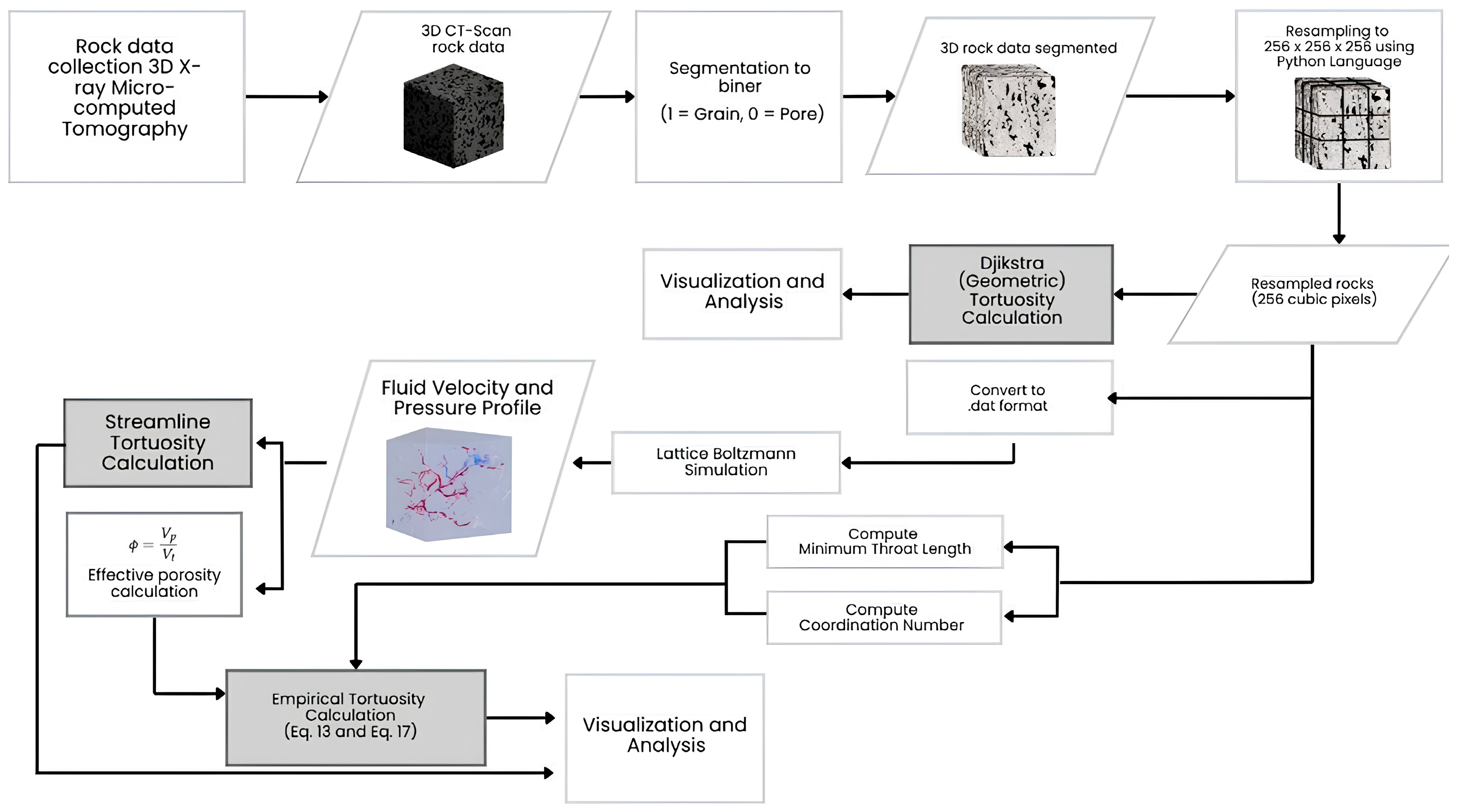
The methodological flowchart in Figure 1 begins with segmentation employing a thresholding technique to convert grayscale images into binary format, thereby enabling the distinction between the matrix phase and the pore space within the rock structure. This thresholding method operates by setting a defined intensity cutoff value: pixels exhibiting intensity values exceeding this threshold are classified as pore space and assigned a white value (1 or 255), whereas pixels with intensity values at or below the threshold are designated as matrix and assigned a black value (0).
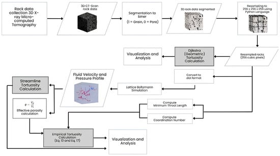
Figure 1.
Methodological flowchart.
By leveraging the contrast in intensity between these two phases, this approach constitutes a critical preprocessing step in image analysis for the quantitative characterization of porous media microstructures.
The grayscale voxel intensity function g(x, y, z) was obtained from 3D micro-CT scans of rock samples. A fixed global threshold of 128, corresponding to the midpoint of the 8-bit grayscale range (0–255), was used to segment pore space (binary value 1) from the solid matrix (value 0). This threshold was selected to ensure consistent segmentation between pore and solid phases, particularly in datasets with bimodal grayscale histograms. The use of a fixed global threshold reduces subjectivity, simplifies the segmentation process, and minimizes the influence of image noise. This approach enhances reproducibility and facilitates direct comparison across multiple samples with varying characteristics.
Each volume was resampled from its original resolution (1000 × 1000 × 1000 voxels) to 256 × 256 × 256 to standardize input for simulation, preserving essential pore-scale features while reducing computational cost. The segmented binary volumes delineate pore and matrix regions and serve as input for finite-volume flow modeling. The dataset comprised 1963 volumes, including 1040 carbonate rock samples (SW01–SW10) and 923 sandstone samples, enabling robust inter-lithology comparisons and high-resolution flow simulations. Tortuosity was subsequently computed to characterize flow path complexity within the pore network (Figure 2), reflecting the deviation of actual flow paths from straight-line trajectories to provide a measure of transport resistance within the porous structure.
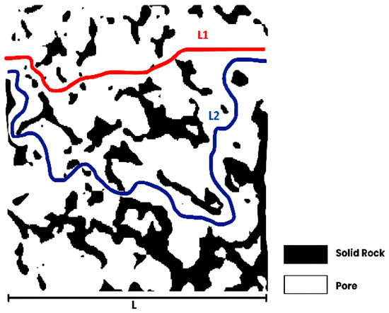
Figure 2.
Fluid flow in porous media: The red line (L1) represents the shortest path, and the blue line (L2) represents the longest path.
Streamline tortuosity offers a more physically representative measure than purely geometric definitions, as it incorporates actual fluid flow behavior. Geological processes such as dissolution, dolomitization, and fracturing introduce heterogeneity and anisotropy, forcing fluids to traverse non-linear, branched pathways within the pore network. As a result, the effective flow path exceeds the straight-line distance between the inlet and outlet boundaries.
Fluid trajectories were computed by integrating the particle motion equation using a fourth-order Runge-Kutta scheme implemented in ParaView 5.9.1 [33]. This better represents the actual behavior of fluid flow in complex porous structures, particularly by capturing the uneven velocity distributions that characterize real flow paths [37] ensuring high numerical accuracy in solving
where denotes the position of a fluid particle at time t, and u is the local velocity vector interpolated from the LBM field. Streamline tortuosity is then defined as the ratio between the streamline length and the straight-line distance and can be solved using the classical fourth-order Runge-Kutta method as follows
This approach captures heterogeneous velocity variations within complex pore geometries, enabling a more accurate representation of fluid flow. Key parameters, including permeability, effective porosity, and tortuosity, are derived from velocity and pressure fields obtained via LBM simulations. The single-phase incompressible fluid flow through the porous medium is governed by the mass and momentum conservation equations,
These equations describe creeping flow characterized by a Reynolds number significantly less than unity. Within porous media, Darcy’s law commonly governs the relationship between flow velocity and pressure gradient, which can be expressed as follows
The LBM functions at the mesoscopic scale by modeling the collective dynamics of particle populations via the particle distribution function f(x, c, t). which represents the probability density of particles possessing velocity c at position x and time t. Macroscopic properties, such as density, are obtained by summing the distribution function over all discrete velocity directions
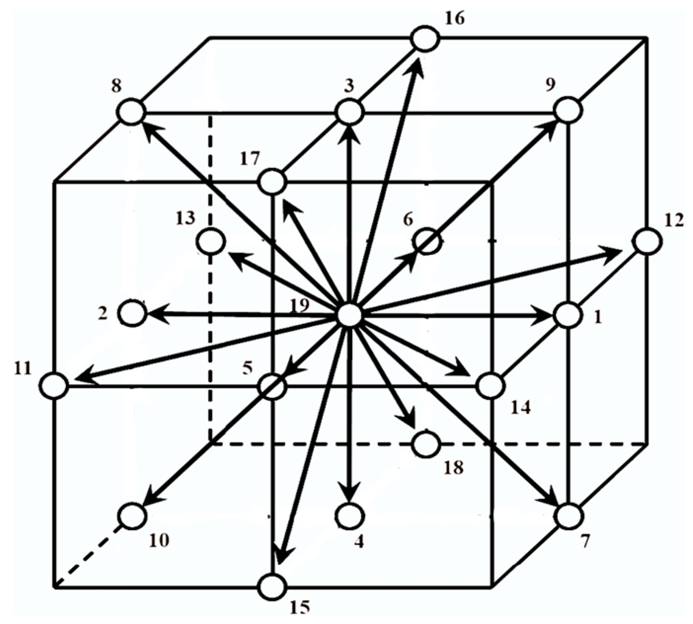
Here, represents the discrete distribution function corresponding to the lattice direction, dependent on spatial position and time. The D3Q19 lattice scheme, depicted in Figure 3, was adopted in this study due to its favorable trade-off between computational cost and solution accuracy.
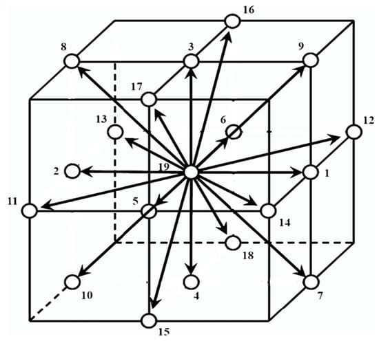
Figure 3.
Discrete velocity in the D3Q19 model scheme.
Table 2 presents the weighting factors for the D3Q19 model. These weighting factors are used in the lattice Boltzmann method to assign relative importance to each discrete velocity direction in the D3Q19 velocity set.
Table 2.
The weighting factor for the D3Q19 model.
This configuration is particularly effective for modeling creeping flow regimes (low Reynolds number) characteristic of fluid transport in porous media. The general LBE is
In the Bhatnagar-Gross-Krook (BGK) model, the evaluation of the particle distribution function at each time step is separated into two primary processes, collision and streaming. The collision mechanism is mathematically represented as follows
where is the equilibrium distribution function and s is the relaxation time. Macroscopic quantities such as density and momentum were computed from the distribution functions as follows
The simulation consisted of streaming and collision steps, with collisions handled via the Single Relaxation Time (SRT) approach based on the BGK model. This method, known for its numerical stability and reduced sensitivity to viscosity, helps suppress spurious velocity fluctuations [38]. Simulations ran for 30,000 time steps ensured steady-state flow with no-slip conditions at the top and bottom walls enforced using the bounce-back scheme. A pressure gradient along the x-direction drove the fluid through the porous domain. The halfway bounce-back condition was applied at solid surfaces as validated in previous studies [39,40]. To minimize numerical slip inherent to BGK models. After reaching convergence, permeability was computed from the velocity and pressure distributions using a Darcy-based formulation adapted for LBM
Effective porosity was estimated from LBM velocity fields using a velocity-thresholding image processing method. Voxels with non-zero velocities were classified as effective pores, while regions with velocities below a threshold were considered ineffective. The threshold was determined as the 10th percentile of the lowest velocity distribution, isolating flow-contributing pores from stagnant zones. A binary mask was generated from this segmentation, and effective porosity was computed using
where is the volume of effective pore space and is the total pore volume. This effective porosity accounts solely for interconnected pores that are actively traversed by the fluid.
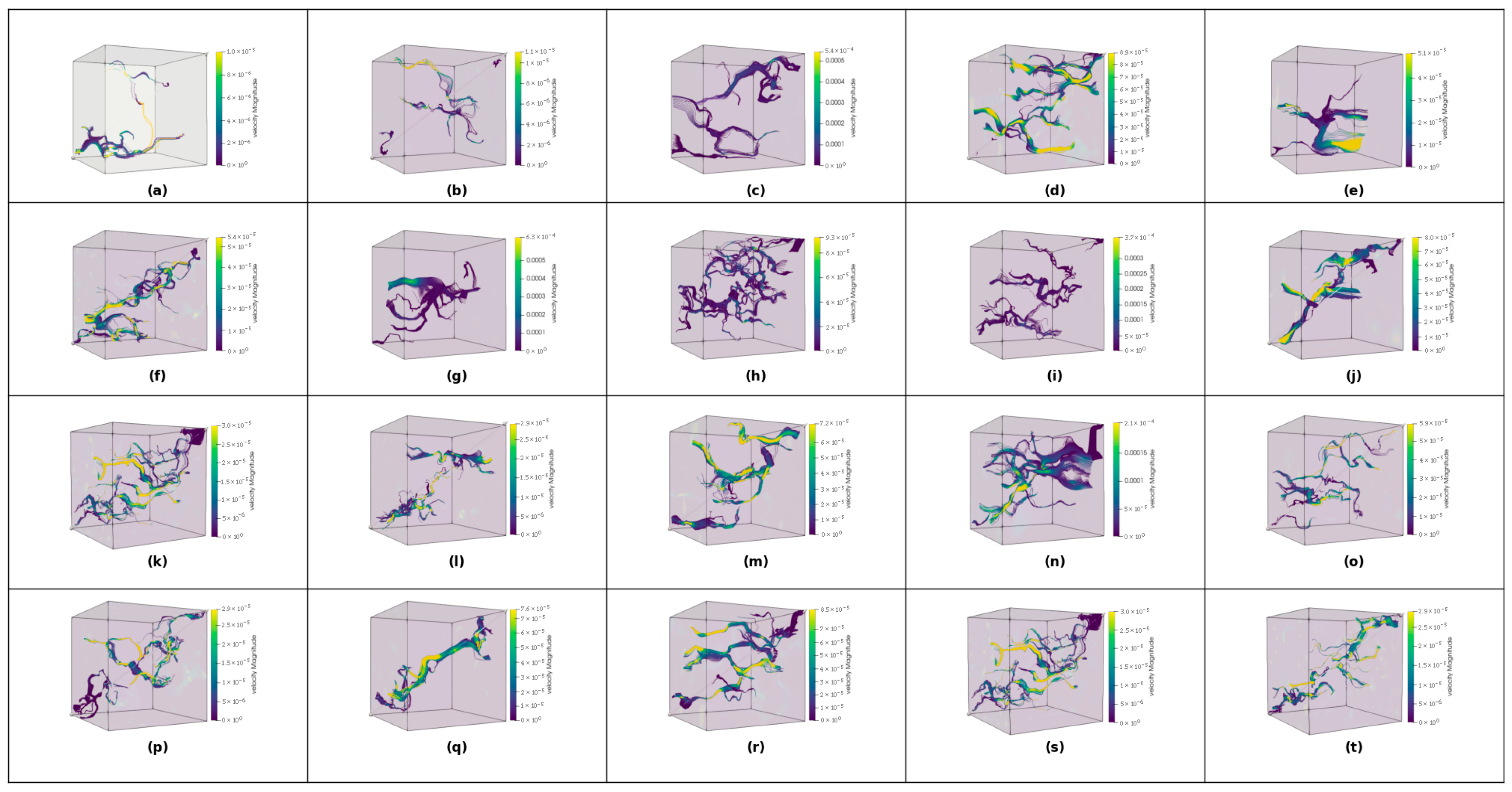
Velocity and pressure gradients were obtained from the LBM simulation and visualized using ParaView 5.9.1 with the stream tracers feature for each rock type. Figure 4 illustrates the fluid flow within each rock sample measuring 256 × 256 × 256 voxels and displays the 3D microstructure of Sandstone and Brazilian pre-salt carbonate rocks, highlighting significant variations in pore distribution and connectivity.
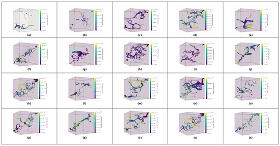
Figure 4.
Velocity field distributions for each sample of rock types. (a) SW01, (b) SW02, (c) SW03, (d) SW04, (e) SW05, (f) SW06, (g) SW07, (h) SW08, (i) SW09, (j) SW10, (k) Bandera Brown, (l) Bandera Gray, (m) Buff Berea, (n) Bentheimer, (o) Berea, (p) BSG, (q) BUG, (r) Castlegate, (s) Kirby, and (t) Leopard.
These microstructural differences form the basis for the quantitative analysis of the relationship between rock physical properties using 3D data.
Geometric tortuosity was computed using Dijkstra’s algorithm, a deterministic weighted shortest-path method applied to the segmented 3D pore structure obtained from micro-CT scans. This algorithm accurately identifies the minimal flow path between inlet and outlet nodes without heuristic approximations, making it well-suited for characterizing tortuous pathways within complex pore networks. Pathfinding was performed in three principal directions, x, y, and z, by identifying whether a connected path exists from one face of the sample to the opposite face through pore voxels only. Once a path is detected, its total length is compared to the straight-line length of the sample in the corresponding direction, yielding the directional tortuosity. The function subsequently returns both the minimum and the average tortuosity across the three directions, thereby determining geometric tortuosity based on the shortest path method.
Geometric tortuosity, , is defined as the ratio of the actual path length of the fluid, , to the straight line distance between the inlet and the outlet, L, and is mathematically expressed as follows
Similar methodologies have been widely adopted in the literature, exemplified by Sun et al. who utilized Dijkstra’s algorithm for pore microstructure characterization [21], and Cecen et al. who applied shortest-path analysis on 3D microstructural datasets of fuel cell materials [40]. These studies reinforce the validity and relevance of this approach in pore structure investigations.
An empirical equation was subsequently employed to corroborate the accuracy of tortuosity estimations encompassing both streamline and geometric aspects. For instance, Avila et al. calculated geometric tortuosity in 3D porous media using the A* algorithm to identify the shortest efficient flow paths [30]. Furthermore, they developed an empirical model capable of predicting geometric tortuosity, τg, solely as a function of the effective porosity of the medium, , which quantifies the fraction of void space available for fluid flow
Additionally, Ghanbarian et al. (2013) proposed a theoretical model for geometric tortuosity [41], expressed as follows
In percolation models of fluid flow in porous media, the occupation probability represents the likelihood that a pore or throat is occupied by fluid, ranging from 0 to 1. The critical occupation probability, pc, marks the threshold for the formation of a continuous flow path. For 3D systems, the correlation length exponent ≈ 0.88 and the fractal dimension of the optimal flow path is . The linear system size is denoted by .
Bernabé et al. [32] showed that there is a linear relationship between the occupation probability and the average pore coordination number Z in regular lattice structures, such as 2D square, hexagonal, and triangular lattices, and 3D simple cubic, body-centered cubic, and face-centered cubic lattices. This relationship underpins the connection between pore network topology and fluid transport properties.
Building on this framework, Ghanbarian et al. improved finite-size scaling by incorporating the coordination number Z [31] and replacing the occupation probability p and the critical threshold with the normalized ratio and , respectively, where is the maximum coordination number.
The scaling constant C is defined as C = 0.85, where represents the minimum tortuous length, corresponding to the shortest pore throat path. This refined scaling approach enhances the accuracy of permeability predictions and improves the reliability of fluid flow modeling in complex porous media.
Subsequently, the values of , , and the minimum throat length () were computed and incorporated into the following equation
The ARE and AICc [42,43] were computed to evaluate the accuracy of the empirical equations and geometric tortuosity as follows
where is the tortuosity value estimated by the model, while τ corresponds to either the geometric tortuosity or the empirical values. N denotes the number of samples, q is the number of input parameters in the model, and RSS is the residual sum of squares. The corrected AICc enables comparison of models with different numbers of parameters, where a smaller AICc indicates a more accurate model.
The tortuosity obtained from the streamline method was used as the ground truth reference to evaluate the accuracy of geometric and empirical tortuosity estimates, ensuring that the benchmark reflects realistic fluid transport pathways within the porous medium. The ARE and AICc were calculated using the streamline-based tortuosity values to quantitatively assess the performance of each model.
Unlike previous studies that examine tortuosity using a single method or limited lithology, this work combines Dijkstra, streamline, and empirical models on 1963 3D images of both carbonate and sandstone rocks, offering a comprehensive comparison framework grounded in LBM-derived flow metrics.
3. Results and Discussion
3.1. Tortuosity Distribution
The tortuosity was evaluated as a key parameter for modeling fluid flow in carbonate and sandstone rocks, utilizing 1963 digital rock samples. Tortuosity was computed using three different approaches: Streamline tortuosity derived from streamlined paths obtained through LBM simulations and used as the reference, geometric tortuosity calculated using Dijkstra’s algorithm, and two empirical models based on macroscopic geometric parameters.
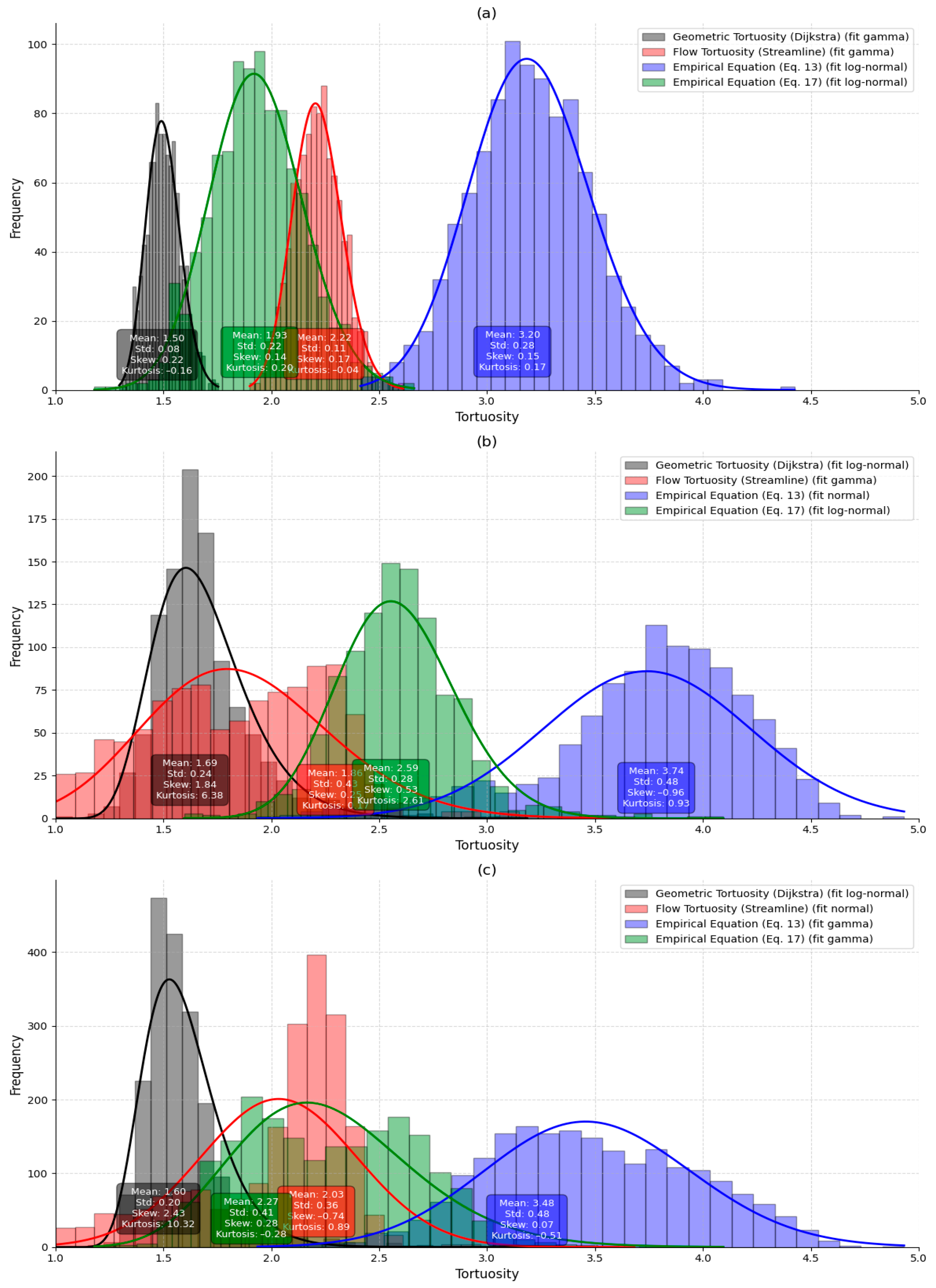
The statistical analysis of tortuosity, as summarized in Figure 5, reveals the distinct behaviors of sandstone and carbonate rocks across Dijkstra, streamline, and empirical tortuosity measures. Distributions were fitted using the best-matching probability functions, gamma, log-normal, and normal, selected based on visual inspection and goodness-of-fit statistics (e.g., skewness, kurtosis, and standard deviation).

Figure 5.
Tortuosity distribution in (a) sandstone, (b) carbonate, and (c) mixed using the Geometric Tortuosity (Dijkstra), Flow Tortuosity (Streamline), and Empirical Equation (Equations (13) and (17)) methods.
The Dijkstra tortuosity of sandstone exhibited a gamma distribution with a mean of 1.50 and a low standard deviation of 0.08. The distribution shows near symmetry, with skewness of 0.22 and slight platykurtosis (kurtosis = −0.16), indicating a relatively homogeneous pore structure. The streamline tortuosity, obtained using the LBM approach, also follows a gamma distribution but with a mean value of 2.22 and a similarly narrow standard deviation of 0.11. Its skewness (0.17) and kurtosis (−0.04) suggest mild asymmetry but overall statistical normality.
The empirical methods yielded more varied results. Tortuosity values calculated using Equation (13) conformed to a log-normal distribution (mean = 1.93, std = 0.22), showing slight positive skewness (0.14) and low kurtosis (0.20), while Equation (17) obtained a significantly higher mean tortuosity of 3.20 (std = 0.28), as well as log-normal distribution with marginal skewness (0.15) and kurtosis (0.17). These differences indicate that empirical estimators may over- or under-predict tortuosity depending on their sensitivity to pore geometry.
Across all tortuosity measures, Dijkstra tortuosity follows a log-normal distribution with a mean of 1.69 and a relatively high standard deviation of 0.24. Its strong positive skewness (1.84) and high kurtosis (6.38) reflect a long-tailed distribution indicative of significant variability in pore path lengths caused by irregular carbonate microstructures. Flow tortuosity modeled via gamma distribution has a mean value of 1.86 with higher variability (std = 0.43), moderate skewness (0.25), and near-normal kurtosis (0.17), suggesting a broader distribution of flow path lengths compared to sandstone.
For empirical models, Equation (17) fitted a log-normal distribution with a mean of 2.59 (std = 0.28), skewness of 0.53, and moderate leptokurtosis (kurtosis = 2.61), while Equation (13) conforms to a normal distribution (mean = 3.74, std = 0.48) with notable negative skewness (−0.96) and slightly elevated kurtosis (0.93). The presence of both left and right-skewed distributions for carbonates highlights the complexity of estimating tortuosity in highly heterogeneous pore systems.
When analyzing the combined dataset across all rock types, the aggregate Dijkstra tortuosity follows a log-normal distribution with a mean of 1.60 and a standard deviation of 0.20. However, its high skewness (2.43) and kurtosis (10.32) point to a strongly right-skewed, heavy-tailed distribution, reinforcing the structural diversity present in carbonate-dominated samples. In contrast, streamline tortuosity fitted a normal distribution (mean = 2.03, std = 0.36), with negative skewness (−0.74) and moderate kurtosis (0.89), suggesting a central tendency with moderate variation, likely due to the averaging effect across lithologies.
The empirical tortuosities exhibit diverse behaviors. Equation (13), fitting a Gamma distribution, yields a mean of 3.48 (std = 0.48), low skewness (0.07), and negative kurtosis (−0.51), reflecting a peaked distribution with limited asymmetry, whereas Equation (17) following a log-gamma distribution has a lower mean of 2.27 (std = 0.41), mild skewness (0.28), and slightly negative kurtosis (−0.28).
The results underscore the greater pore-scale complexity of carbonate rocks compared to sandstones, particularly in the Dijkstra and streamline tortuosity statistics. The pronounced skewness and kurtosis in carbonates indicate irregular, anisotropic flow paths that are not well captured by empirical equations alone. Among the evaluated methods, the LBM-derived flow tortuosity appears most representative of true flow behavior due to its sensitivity to microstructural heterogeneity, making it the preferred approach for accurate modeling of transport properties in porous media.
3.2. Tortuosity Comparison Across Streamline
The streamlined geometric tortuosity values in Figure 6 were used as a reference (ground truth) and plotted on the y-axis against various tortuosity estimates obtained from alternative methods.
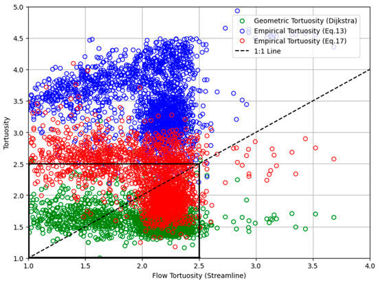
Figure 6.
Tortuosity estimated values from Dijkstra, Equation (13) by Ávila et al. [30] and Equation (17) of the proposed percolation-based model are plotted against the streamline on the x-axis.
The tortuosity values based on the streamline method range from 1.0 to 2.5, generally reflecting the complexity of fluid flow paths within the rock pores. Notably, the Dijkstra method and the semiempirical approach formulated in Equation (17) are consistent with the streamline values, with most data points closely distributed around the 1:1 reference line, depicted by the solid line in Figure 6. This indicates that both approaches can accurately represent the actual flow paths in porous media.
In contrast, the tortuosity estimates derived from Equation (13) significantly deviated from the ground truth, with widely scattered values reaching 5.0, suggesting a high sensitivity to the input parameters used in that formulation. Specifically, Equation (13) relies solely on the effective porosity of the rock samples, which appears insufficient to capture the geometric and topological complexities of the pore pathways in heterogeneous porous media. By comparison, the formulation in Equation (17) is more comprehensive, integrating several key microstructural parameters known to influence transport behavior.
These parameters include effective porosity, the average coordination number , the maximum coordination number relative to the average (), and the minimum throat length () within the pore network. Following the approach proposed by Ghanbarian et al., the empirical coefficient C is set to [44] to align the estimation with local geometric characteristics represented by the minimum throat length, which physically corresponds to the lower bound of flow resistance within the rock pores. Overall, these results underscore the importance of a multiparametric approach for accurately estimating Dijkstra tortuosity. Incorporating additional pore network structural information enhances prediction accuracy, ultimately providing a more realistic depiction of fluid flow dynamics within complex porous media. This is especially relevant at the microscopic scale, which is critical for transport studies in geological systems and reservoir engineering.
3.3. Boxplot of Tortuosity Values by Porosity Group (L1–L5)
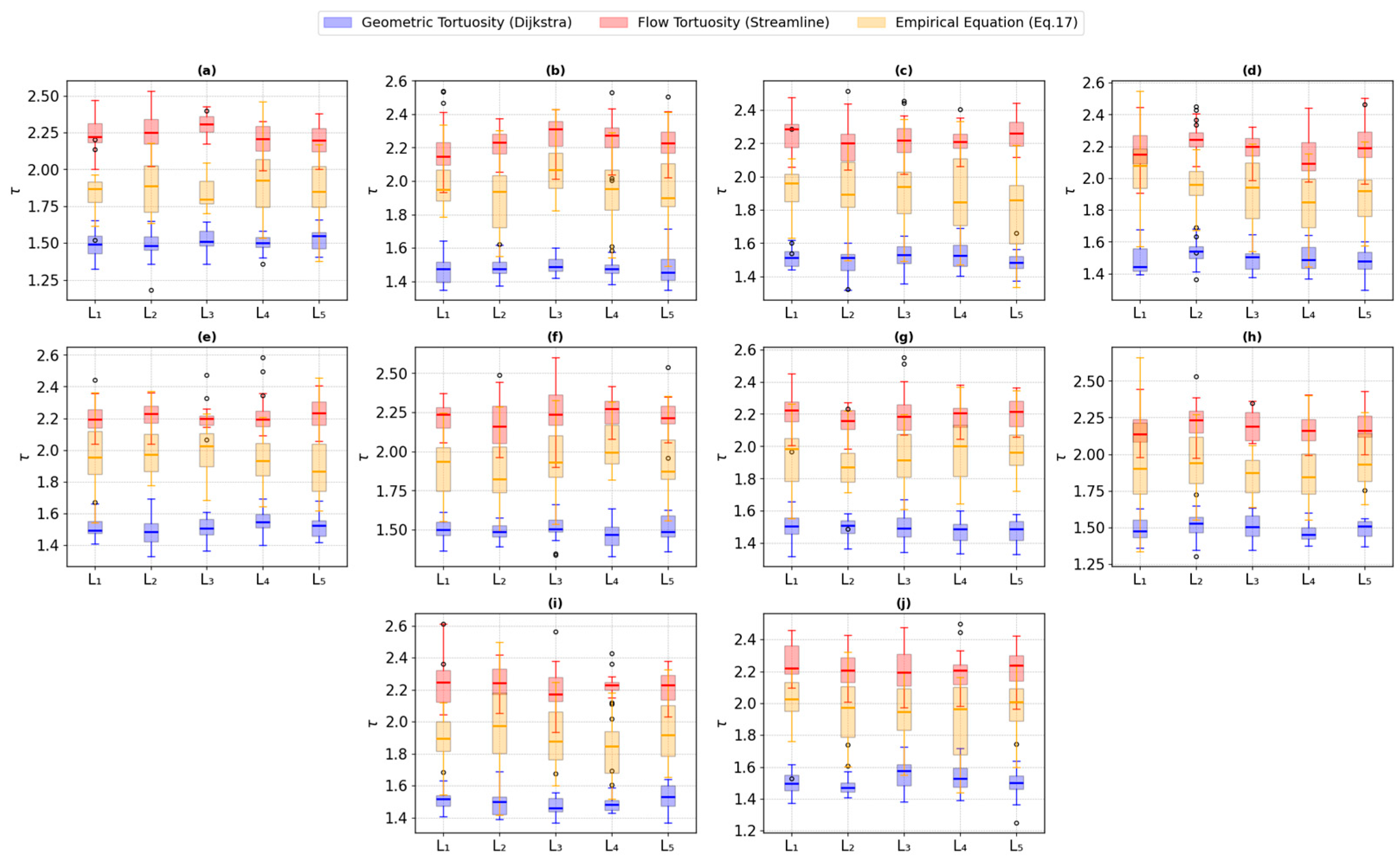
To evaluate the consistency of the relationship between porosity and tortuosity across different rock types, box plots in Figure 7 and Figure 8 were employed to visualize the variation in tortuosity as a function of grouped porosity values. Porosity was discretized into five categorical groups, labeled L1 to L5, arranged from the lowest (L1) to the highest (L5) porosity interval, with each group representing 20% of the porosity distribution to balance statistical robustness and resolution, ensuring meaningful comparisons while covering the observed porosity spectrum. The five-bin grouping aligns with conventional quantile-based methods in porous media studies, enabling comparisons with prior research. Each boxplot displays tortuosity (y-axis) calculated by three methods: Dijkstra’s algorithm, streamline tortuosity, and an empirical model represented by Equation (17).
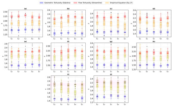
Figure 7.
Tortuosity of sandstone samples (a) Bandera Brown, (b) Bandera Gray, (c) Buff Berea, (d) Bentheimer, (e) Berea, (f) Berea Sister Gray, (g) Berea Upper Gray, (h) Castlegate, (i) Kirby, and (j) Leopard.
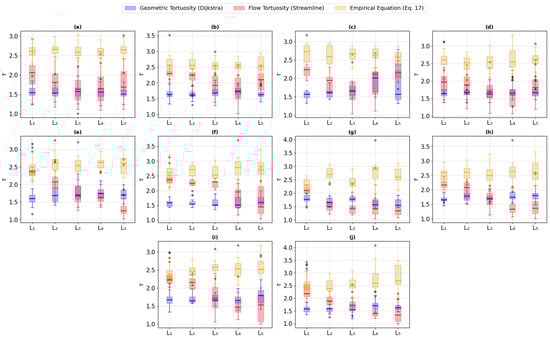
Figure 8.
Tortuosity of carbonate samples (a) SW01, (b) SW02, (c) SW03, (d) SW04, (e) SW05, (f) SW06, (g) SW07, (h) SW08, (i) SW09, and (j) SW10.
Preliminary evaluations showed that the predictions significantly deviated from both simulation-based results and the observed empirical behavior. Equation (13), although widely cited, tends to under- or overestimate tortuosity under certain pore geometries, particularly in heterogeneous formations like carbonates; thus, it is less representative of actual tortuosity under the studied conditions and was therefore omitted from detailed interpretation. The selection of Dijkstra, streamline simulation, and Equation (17) ensures that structural and flow-related mechanisms are captured while maintaining a tractable and reliable empirical reference, providing a comprehensive framework for understanding tortuosity variations across lithologies and validating the robustness of porosity-tortuosity trends in porous media.
The x-axis categorizes samples by their porosity (L1–L5), revealing clear distinctions between sandstone and carbonate lithologies. Sandstone samples exhibit more homogeneous behavior, with relatively stable tortuosity values and consistent distributions across porosity groups. This homogeneity is evident in the tighter and more symmetric boxplot spreads, indicating uniform pore structures and flow pathways within sandstones. In contrast, carbonate samples display far greater variability in tortuosity values, especially for streamline tortuosity and Dijkstra tortuosity derived from simulations of actual rock structures. The widespread and irregular distribution of data points highlights the inherently heterogeneous pore geometry and complex flow networks typical of carbonates.
Interestingly, tortuosity values estimated from the empirical model using Equation (17) tend to be more stable even for carbonates, suggesting that empirical correlations may smooth out microstructural heterogeneities that significantly affect simulation-based methods. These findings underscore the difference in pore-scale complexity between sandstones and carbonates and validate the use of porosity grouping as a useful framework for comparative analysis. The more homogeneous sandstone behavior contrasts with the heterogeneous carbonate response, providing important insight into how lithological variability influences tortuosity-porosity relationships and porous media flow physics.
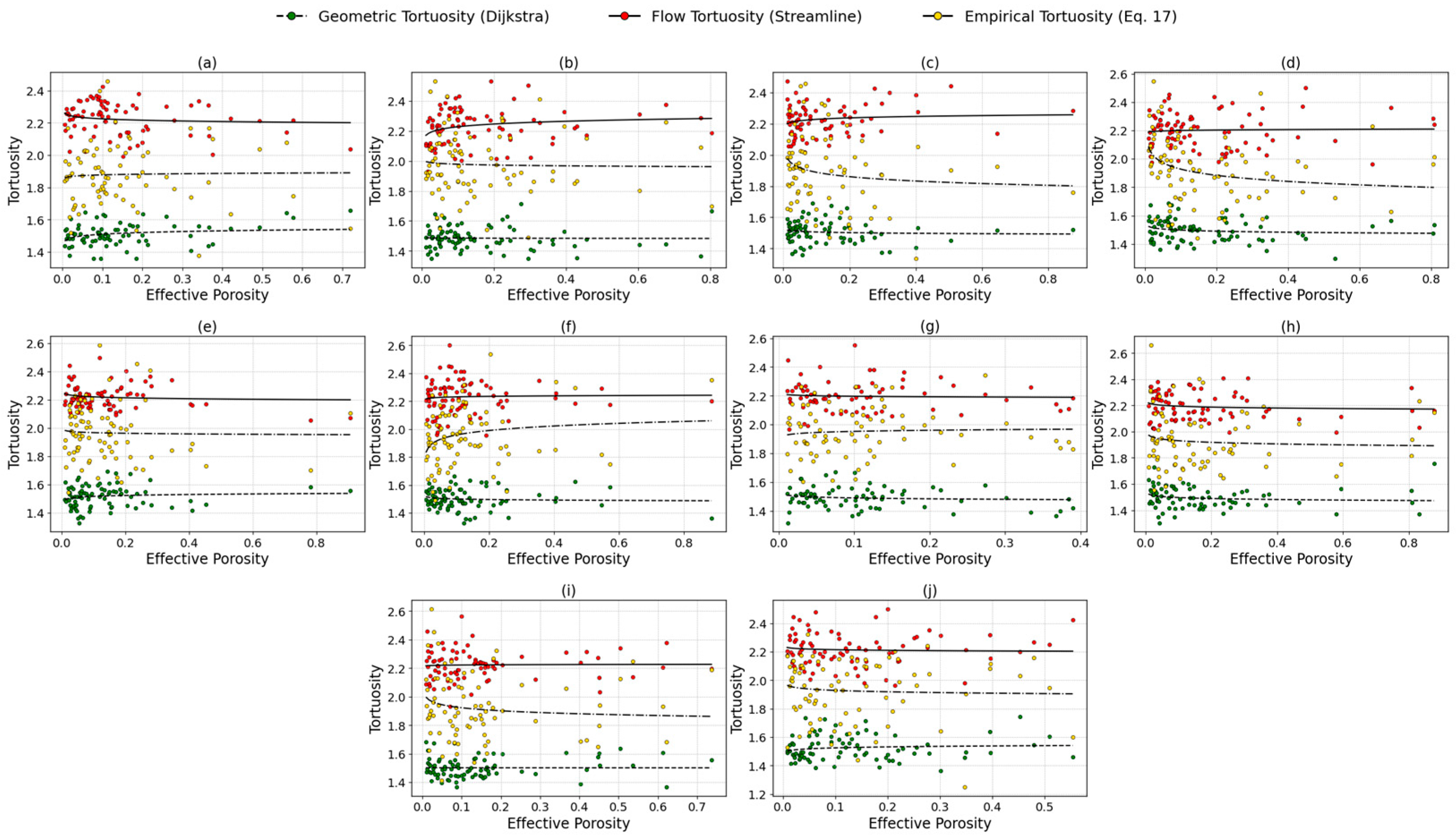
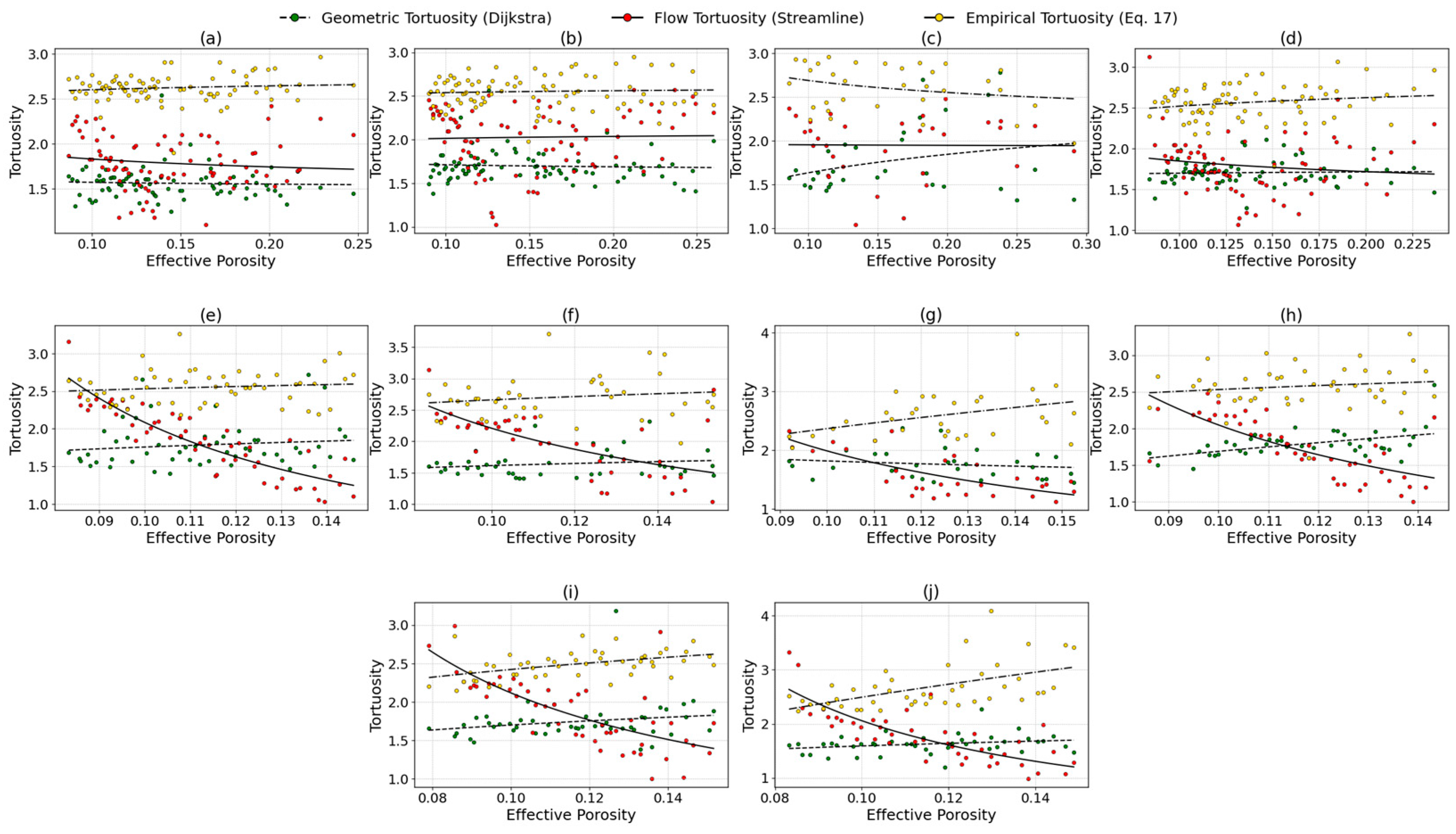
3.4. Tortuosity-Porosity Relationship
Figure 9 and Figure 10 illustrate the relationship between tortuosity and effective porosity for sandstone and carbonate rock samples, respectively. In Figure 9, which represents sandstone rocks, the tortuosity values estimated by the streamline method, Dijkstra, and empirical approach Equation (17) are generally consistent and fall within a similar range across varying porosity values.
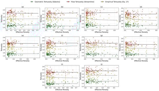
Figure 9.
Tortuosity-porosity relationship of in sandstone samples (a) Bandera Brown, (b) Bandera Gray, (c) Buff Berea, (d) Bentheimer, (e) Berea, (f) Berea Sister Gray, (g) Berea Upper Gray, (h) Castlegate, (i) Kirby, and (j) Leopard.
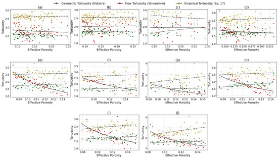
Figure 10.
Tortuosity-porosity relationship of carbonate samples (a) SW01, (b) SW02, (c) SW03, (d) SW04, (e) SW05, (f) SW06, (g) SW07, (h) SW08, (i) SW09, and (j) SW10.
Most data points are densely clustered within an effective porosity interval of 0.001 to 0.4, indicating a stable agreement among the three methods. This consistency suggests that in relatively homogeneous porous structures like sandstones, Dijkstra and empirical models can approximate the streamline tortuosity with reasonable accuracy.
In general, Equation (17) yielded the highest average coefficient of determination (R2) among the three approaches for fitting the relationship between tortuosity and porosity in sandstone samples, although the value was relatively low at approximately 0.023. For the Dijkstra method, the highest R2 was observed in the Bandera Brown rock, while the lowest values were found in Bandera Gray and Kirby. The streamline method obtained the highest R2 in Bandera Gray at 0.049, whereas the lowest was in Kirby (0.001). The best fit achieved by Equation (17) was in the Bentheimer rock (R2 = 0.096), while the poorest fit occurred in the Berea rock (R2 = 0.001). In contrast, there were significant discrepancies in carbonate rock samples between streamline-based tortuosity and those estimated using Dijkstra and the empirical equation (Figure 10). Overall, the streamline method provided the best fit (R2 = 0.348), while the geometric method showed the poorest agreement. The lowest R2 for Dijkstra was observed in sample SW04 (0.001), and the highest in SW08 (0.230). For the streamlined approach, R2 ranged from 0.000 (SW03) to 0.794 (SW05), while the empirical method had a range from 0.003 (SW02) to 0.281 (SW10).
The pronounced deviation of streamline tortuosity reflects the complex and heterogeneous pore structure of carbonate rocks, where features such as vugs, irregular throats, and disconnected pore clusters significantly influence fluid flow. In such systems, geometric and empirical models often fail to capture the true transport pathways; therefore, streamline approaches, such as the lattice Boltzmann method, are critical to accurately quantifying tortuosity in rocks with substantial pore-scale variability. This highlights the limitations of applying generalized models across lithologically diverse media.
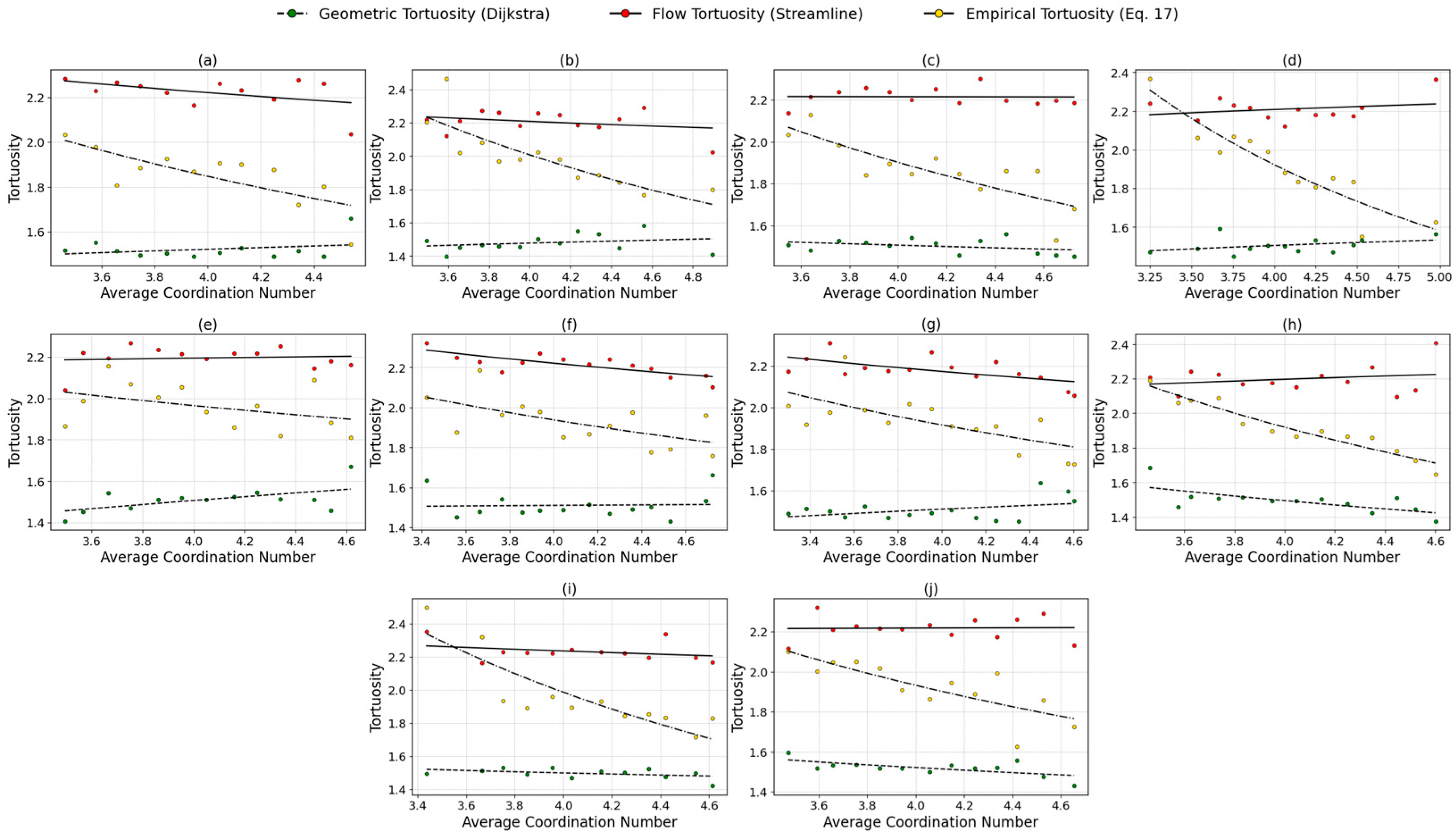
3.5. Tortuosity-Average Coordination Number Relationship
Figure 11 and Figure 12 illustrate the relationship between tortuosity and average coordination number for sandstone and carbonate rocks, respectively. This plot was constructed because is directly involved in one of the empirical equations used to estimate tortuosity. A higher generally indicates better pore connectivity which may reduce the effective flow path length, thereby lowering tortuosity. Conversely, lower coordination numbers often correspond to more isolated or poorly connected pores, potentially increasing the tortuosity of the medium.
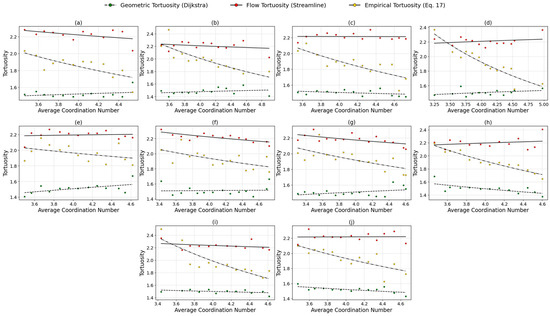
Figure 11.
Tortuosity-average coordination number relationship in sandstone samples (a) Bandera Brown, (b) Bandera Gray, (c) Buff Berea, (d) Bentheimer, (e) Berea, (f) Berea Sister Gray, (g) Berea Upper Gray, (h) Castlegate, (i) Kirby, and (j) Leopard.
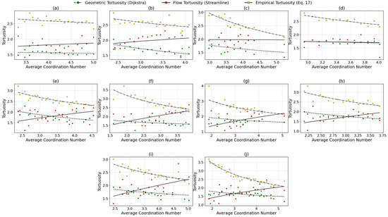
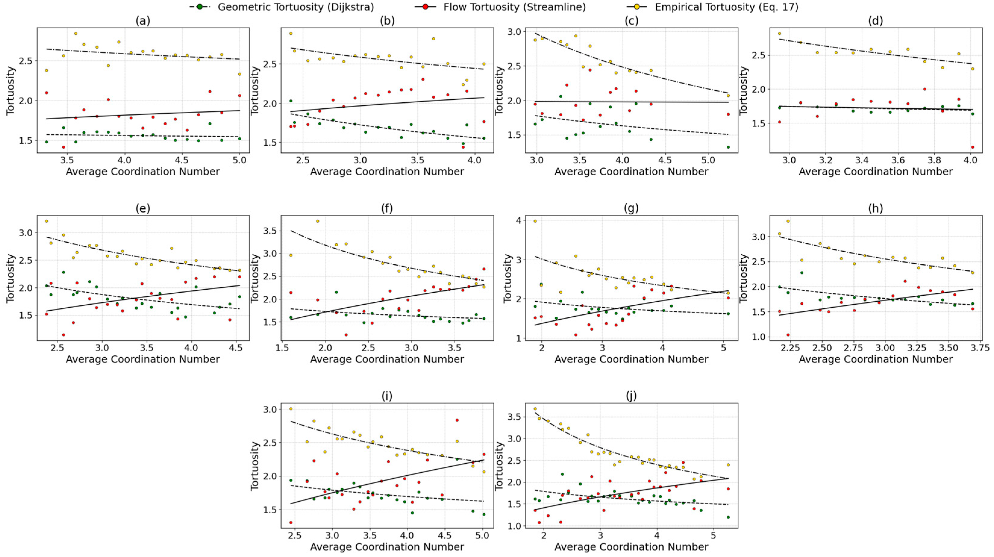
Figure 12.
Tortuosity-average coordination number relationship in carbonate samples (a) SW01, (b) SW02, (c) SW03, (d) SW04, (e) SW05, (f) SW06, (g) SW07, (h) SW08, (i) SW09, and (j) SW10.
A clear inverse correlation was observed in sandstones (Figure 11), particularly in the empirical tortuosity values derived from Equation (17). Overall, the best fit was achieved using Equation (17), with an average R2 of 0.609, while the lowest was observed for the streamline method, at 0.148. For the Dijkstra method, the lowest R2 occurred in Berea Sister Gray, and the highest in Castlegate (0.465). In comparison, the lowest R2 was found in Buff Berea, and the highest in Berea Sister Gray (0.592) for the streamline-based tortuosity. The R2 ranged from 0.159 (Berea) to 0.917 (Castlegate) for Equation (17).
As tortuosity increases, the average decreases significantly, supporting the theoretical expectation that higher tortuosity—representing more convoluted flow paths—is associated with lower pore connectivity. This trend was also observed, though less distinctly, in both the streamline and Dijkstra-derived tortuosity values, which show a more gradual decline in with increasing tortuosity. The consistency of this inverse relationship across methods, particularly evident in Equation (17), confirms the structural coherence of sandstone pore networks, where variations in local coordination are effectively captured by tortuosity metrics. We aim to validate the physical consistency of the empirical model by examining this relationship, further exploring how topological features of the pore structure influence fluid transport behavior.
In contrast, carbonate rocks (Figure 12) exhibit a more complex and less predictable relationship. While the Dijkstra and Equation (17) tortuosity values demonstrate a marked inverse correlation with coordination number—similar to that observed in sandstones—the streamline-based tortuosity reveals a divergent pattern. Here, tortuosity and appear to be positively correlated, indicating that samples with higher streamline tortuosity may also exhibit higher average connectivity. Overall, the best fitting performance was observed for the empirical method Equation (17), with an average Overall, the best fitting performance was observed for the empirical method Equation (17), with an average R2 of 0.585, while the lowest was found in the streamline method, with an average R2 of 0.205. For the Dijkstra method, the lowest R2 was obtained for sample SW01 (0.016), and the highest for SW02 (0.616). In the streamline method, the lowest value occurred in SW03, while the highest was in SW08 (0.435). For the empirical model Equation (17), R2 ranged from 0.092 in SW01 to 0.916 in SW10.
This seemingly counterintuitive trend indicates that tortuosity derived from flow simulations is influenced not only by geometric connectivity in carbonate systems but also by localized features such as constrictions, dead ends, and preferential high-velocity channels. These characteristics, typical of carbonate pore structures, increase flow complexity despite well-connected networks and reflect the fundamental pore-structure differences between sandstones and carbonates. The strong inverse correlation observed in sandstones supports their relatively uniform granular framework, where the average coordination number (), but also reliably correlates with tortuosity across different estimation methods. Conversely, in carbonates, the greater pore-type diversity and spatial heterogeneity disrupt the direct relationship between coordination number and flow behavior, limiting the effectiveness of empirical or geometric Z metrics in capturing flow complexity.
These results highlight the necessity of considering both pore connectivity and dynamic flow processes when assessing tortuosity in heterogeneous media. While remains a valuable structural parameter, its predictive power for transport properties varies with rock type and the method of tortuosity estimation. Therefore, integrating multiple characterization approaches is essential for accurately modeling fluid transport in complex porous systems.
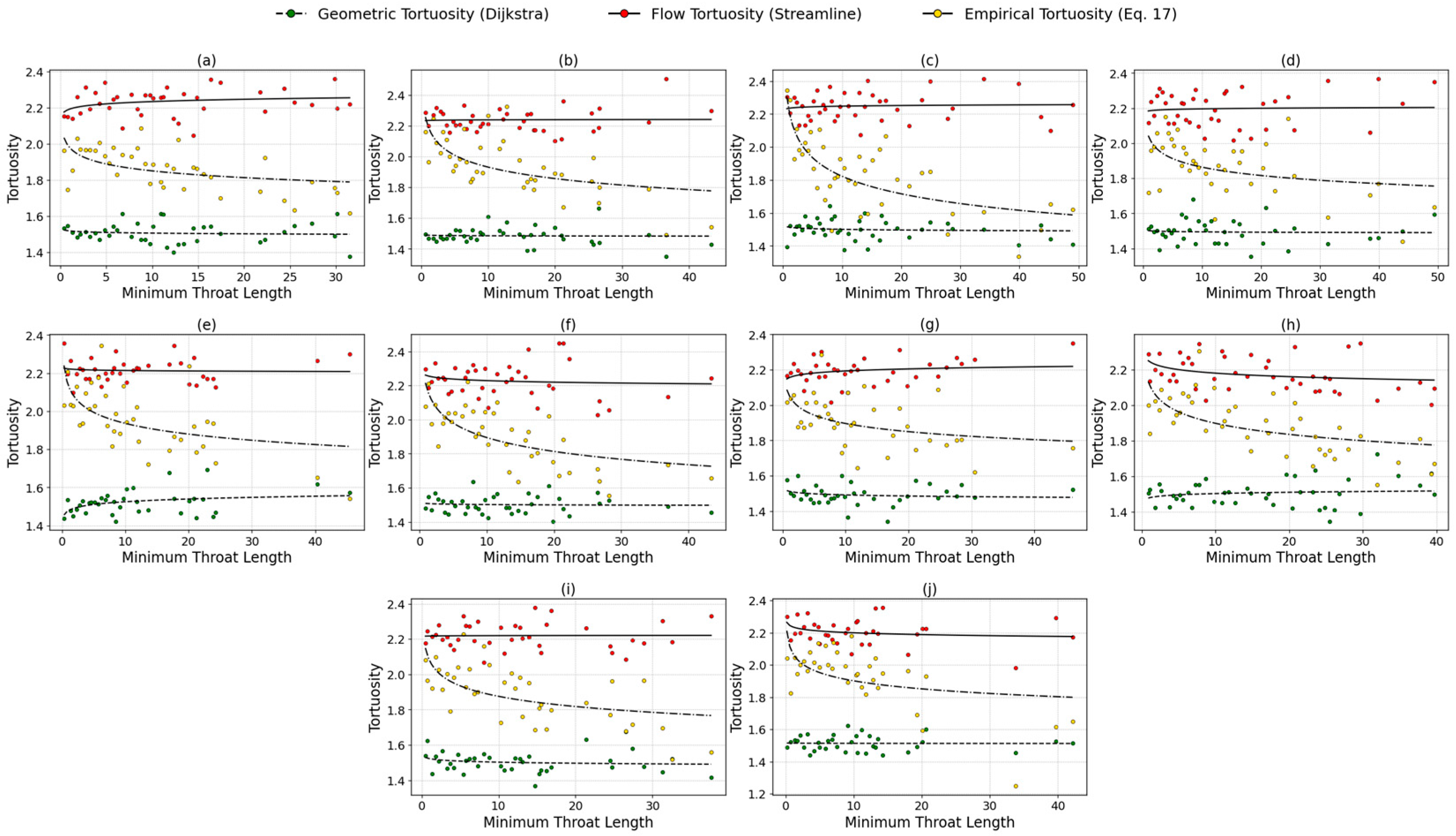
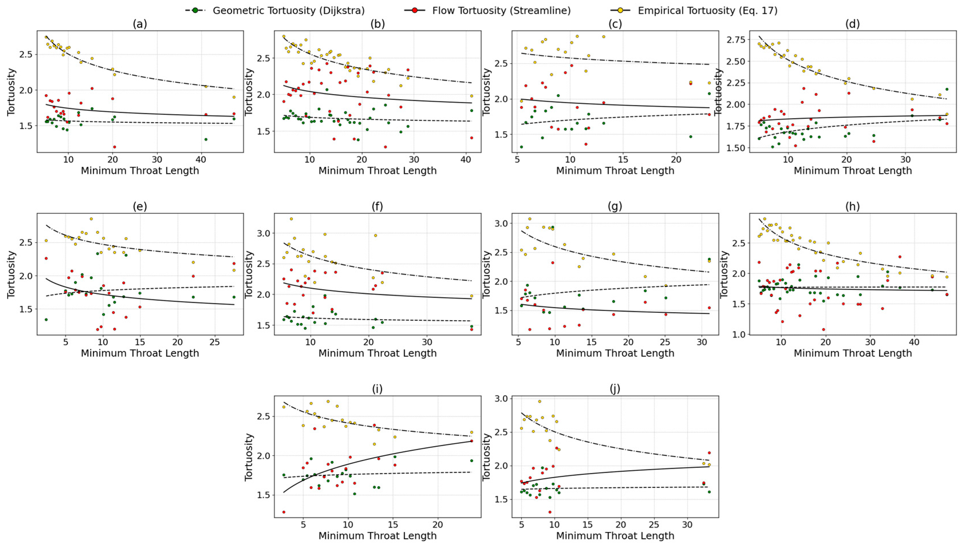
3.6. Tortuosity-Minimum Throat Length Relationship
Figure 13 and Figure 14 present the relationship between tortuosity and minimum throat length for sandstone and carbonate rocks, respectively.
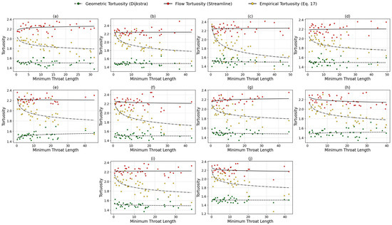
Figure 13.
Tortuosity-minimum throat length relationship of sandstone samples (a) Bandera Brown, (b) Bandera Gray, (c) Buff Berea, (d) Bentheimer, (e) Berea, (f) Berea Sister Gray, (g) Berea Upper Gray, (h) Castlegate, (i) Kirby, and (j) Leopard.
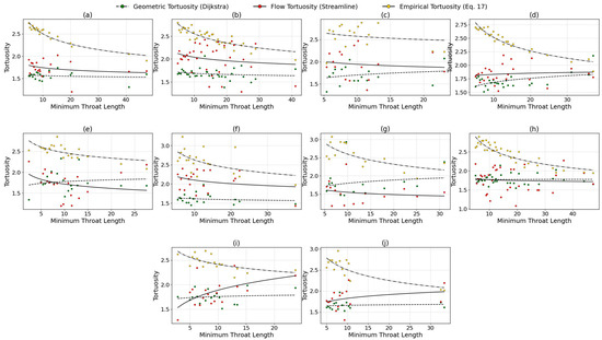
Figure 14.
Tortuosity-minimum throat length relationship of carbonate samples (a) SW01, (b) SW02, (c) SW03, (d) SW04, (e) SW05, (f) SW06, (g) SW07, (h) SW08, (i) SW09, and (j) SW10.
The tortuosity values of sandstone samples analyzed using Equation (17) decrease as the minimum throat length increases. This trend is particularly evident in both the streamline and Dijkstra methods, where the tortuosity values remain relatively stable and approximately linear, indicating a consistent flow path complexity relative to pore constrictions. This behavior suggests that in sandstone formations, larger minimum throat lengths correspond to simpler, less tortuous flow paths, consistent with the expected pore geometry where wider throats facilitate more direct fluid transport. The observed linearity in tortuosity for both the streamline and Dijkstra methods further supports their robustness in capturing the geometric constraints imposed by throat sizes in porous sandstone.
The best fitting performance was obtained using Equation (17), with an average R2 of 0.328, while the lowest was found in the Dijkstra method, with an average R2 of 0.022. For the Dijkstra method, the lowest R2 was observed in Bandera Gray (0.001), and the highest in Berea (0.130), whereas for the streamline method, the lowest R2 values were recorded in Bandera Gray and Kirby, while the highest was found in Castlegate (0.090). For Equation (17), the lowest R2 was observed in Bentheimer (0.196), and the highest in Buff Berea (0.553).
Conversely, carbonate rocks (Figure 14) exhibited an inverse relationship, where higher tortuosity values tend to correspond with smaller minimum throat lengths, suggesting that narrow pore throats significantly contribute to the increased complexity of flow paths. Such behavior likely results from the inherently heterogeneous and anisotropic pore structures characteristic of carbonate formations, where restricted flow through smaller throats forces fluids to navigate more winding and tortuous pathways. Consequently, tortuosity increases as minimum throat size decreases, reflecting greater flow path complexity and resistance.
The best fitting performance was observed with Equation (17), yielding an average R2 of 0.554, while the lowest was obtained using the Dijkstra method, with an average R2 of 0.041. For Dijkstra, the lowest R2 was recorded in sample SW08, and the highest in SW04 (0.221), with the R2 values ranging from 0.004 (SW08) to 0.289 (SW09). For Equation (17), the highest R2 was found in SW01, and the lowest in SW03 (0.030).
However, notable deviations from this general trend were observed in the streamline-derived tortuosity for samples SW05 and SW09, as well as in the Dijkstra-based tortuosity for sample SW07, where an increase in tortuosity coincides with an increase in minimum throat length. This behavior may be attributed to distinct pore-scale features or heterogeneities present in these specific samples, such as poorly connected throats or nonuniform throat size distributions. Such characteristics can result in more tortuous flow paths despite the presence of larger minimum throat dimensions, underscoring the complex and non-linear relationship between geometric parameters and effective flow tortuosity in heterogeneous carbonate rocks. Overall, these findings highlight the contrasting pore-scale flow dynamics between sandstone and carbonate rocks, with sandstone exhibiting a more straightforward dependency of tortuosity on the minimum throat length.
This is due to the intricate dependence of flow tortuosity on pore connectivity, topological order, and microscale anisotropy, factors not fully captured by porosity alone. Consequently, samples with identical effective porosities can have vastly different internal architectures, resulting in significantly varied flow path lengths. Therefore, while effective porosity filters out non-conductive pore spaces, it alone cannot represent the spatial complexity of flow paths characterized by flow tortuosity.
3.7. Comparison of Tortuosity Studies
A comparative analysis with previous experimental and numerical investigations on similar porous materials was conducted to assess the validity of the tortuosity values obtained in this study (Table 3).
Table 3.
Comparison of tortuosity studies across various porous media and methods. Porosity values are explicitly categorized as either absolute or effective porosity, where reported. Flow tortuosity values are based on direct fluid simulations. Dijkstra tortuosity values are typically obtained from shortest path algorithms.
Koponen et al. investigated 2D synthetic porous media using the lattice-gas automata method (FHP-III model) to examine the empirical relationship between tortuosity and porosity [45]. Analytical methods were found to be inadequate for capturing the complexity of fluid transport in such systems, prompting the use of direct numerical simulations. Their results indicated that the flow tortuosity varied between 1.1 and 1.7 within a porosity range of 0.4 to 0.9. There was a correlation between increasing tortuosity and decreasing porosity, highlighting the nontrivial nature of pore-scale connectivity in controlling transport behavior. Panini et al. reported geometric tortuosity values between 1.00 and 1.80 for sandstone and carbonate samples within a porosity range of 0.07 to 0.37, whereas the empirical tortuosity values derived from correlation-based models showed a broader distribution from 1.00 to 7.00. This suggests that while empirical models are highly sensitive to variations in pore structure, they may produce significant deviations if not calibrated carefully to internal geometrical features. A recent study by Nurcahya et al. [26] analyzed 2D representations of sandstone and found geometric tortuosity ranging from 1.38 to 2.20 across effective porosities of 0.06 to 0.325. In a follow-up study conducted in 2025, the same group extended their investigation to 3D models (128 × 128 × 128 voxels) and reported flow tortuosity values ranging from 2.25 to 3.75 for effective porosities between 0.05 and 0.35. These findings support theoretical expectations, as the transition from two to three dimensions typically leads to greater complexity in flow paths due to enhanced connectivity and geometric constraints. In the present study, the tortuosity values observed for 3D sandstone samples with effective porosity from 0.08 to 0.22 were in good agreement with these prior reports: geometric tortuosity ranged from 1.29 to 1.75, flow tortuosity from 1.18 to 2.61, and empirical tortuosity estimates were between 2.47 to 4.42 for Equation (13) and 1.18 to 2.59 for Equation (17). For carbonate samples, which are known for their greater heterogeneity and structural complexity, the effective porosity ranged from 0.03 to 0.30 with geometric tortuosity values ranging from 1.00 to 3.18, flow tortuosity from 1.00 to 3.68, and empirical tortuosity from 2.45 to 4.93 for Equation (13) and 1.59 to 3.47 for Equation (17). The wider spread in empirical estimates reflects the high sensitivity of such models to input parameters, highlighting their limitations in capturing complex microstructures without proper adjustment. Overall, these findings emphasize the relevance of using a combination of geometric, fluid streamline, and empirical methods for tortuosity characterization, providing valuable insight into transport behavior within natural porous systems of varying lithological and structural characteristics.
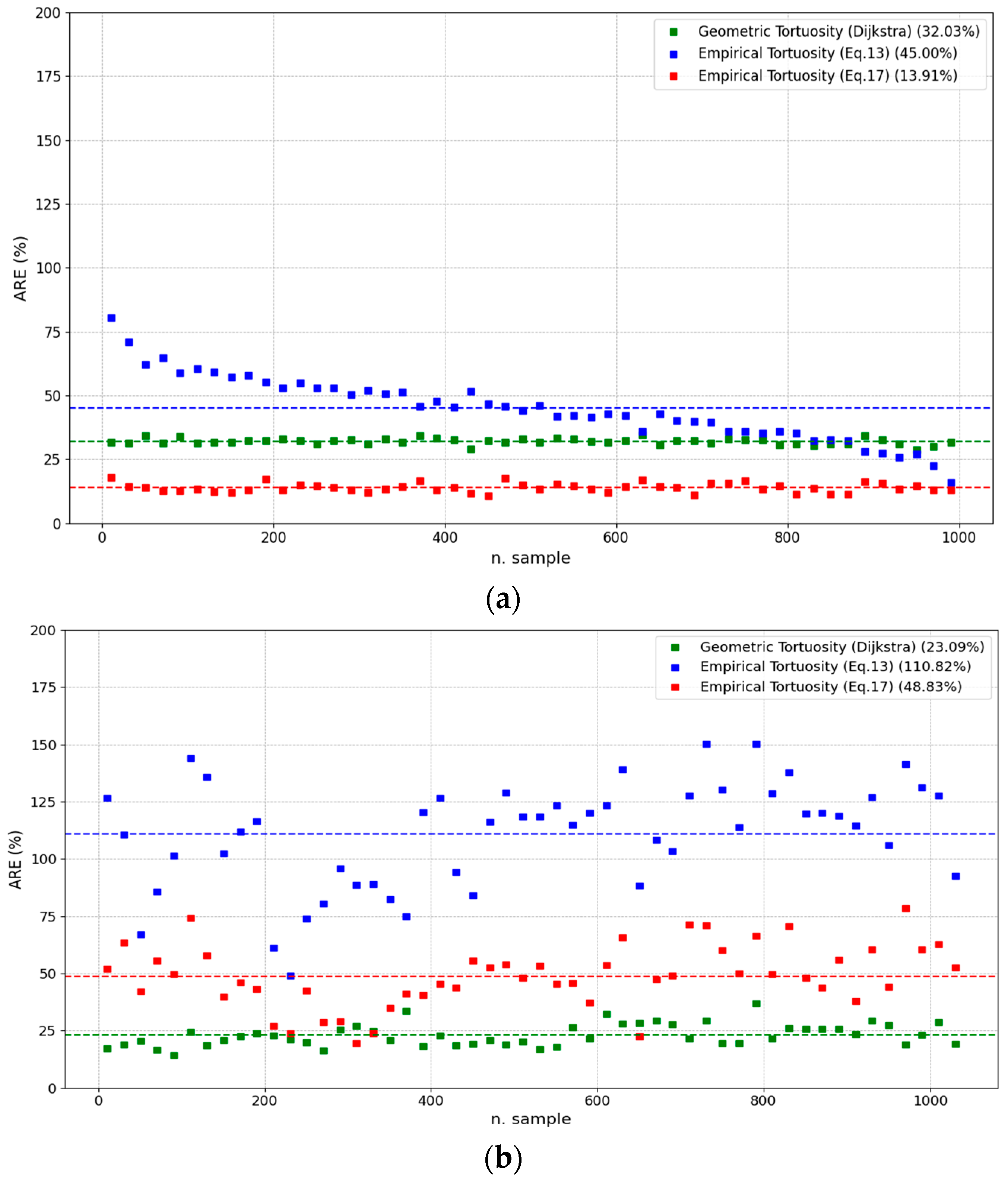
3.8. ARE
Absolute Relative Error (ARE) as the primary metric for performance evaluation, representing the proportional deviation of estimated tortuosity from streamline-based reference values. This formulation ensures scale-independence and enables robust inter-method comparisons. Figure 15a presents the ARE for the sandstone samples, using streamline tortuosity obtained from streamline simulations as the ground truth for comparison.
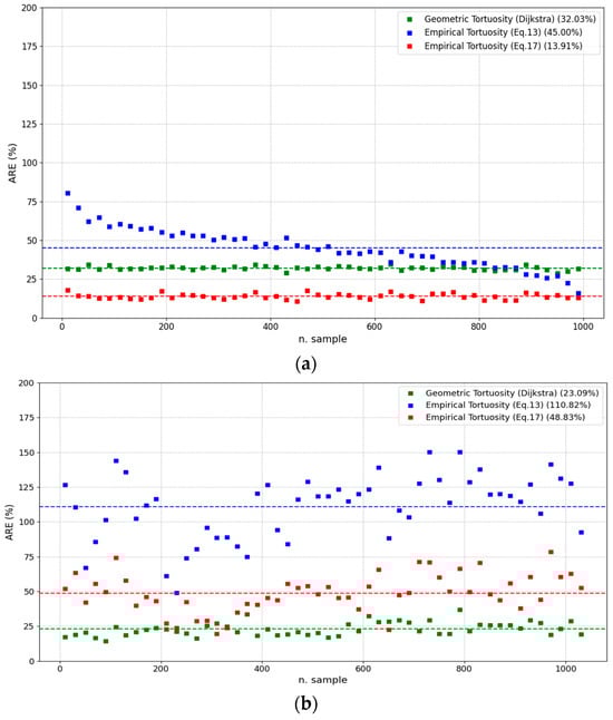
Figure 15.
ARE of (a) sandstone and (b) carbonate samples.
Equation (17) exhibits the highest predictive accuracy with an ARE of 13.91%, effectively capturing the dominant flow paths in sandstone, which typically feature a relatively homogeneous and well-connected pore structure. In contrast, the Dijkstra method and Equation (13) exhibit significantly larger discrepancies, with ARE values of 32.03% and 45.00%, respectively, suggesting that the assumptions or sensitivities underlying these models may not be well-suited to the simpler and more uniform sandstone geometry. Specifically, while the Dijkstra algorithm considers the shortest paths through the medium, it may overestimate or underestimate tortuosity in systems where flow is more uniformly distributed across the pore space. Meanwhile, Equation (13) relies solely on porosity, which likely limits its ability to capture the actual pore structure and connectivity. These findings confirm that Equation (17) offers a robust and efficient estimation of streamline tortuosity for relatively homogeneous porous media such as sandstone.
Figure 15b shows that Equation (13) yields a very high ARE of 110.82% for carbonate rocks, indicating a substantial deviation from the streamline-derived tortuosity and a fundamental misrepresentation of the actual flow pathways. This underperformance likely stems from the model’s limited ability to account for the intricate and highly heterogeneous pore systems typical of carbonate rocks.
In contrast, Equation (17) and the Dijkstra algorithm exhibit superior performance, with AREs of 48.83% and 23.09%, respectively, attributed to their better adaptability to complex pore networks, where connectivity, tortuous paths, and dead-end pores are prevalent. Dijkstra’s algorithm traces the most efficient path from inlet to outlet within a voxelized pore space; thus, it is inherently sensitive to variations in pore geometry and spatial heterogeneity, making it more suitable for modeling flow in such systems.
These results underline the importance of model selection based on lithological characteristics and pore architecture complexity. Taken together, the contrasting performances of the models across sandstone and carbonate samples indicate that no single model provides universally accurate tortuosity predictions across different rock types. While Equation (13) demonstrates satisfactory performance in systems characterized by relatively regular and continuous pore networks, such as high-porosity sandstones, its application to more complex and heterogeneous media, such as carbonate rocks, results in notable discrepancies. Its underlying assumptions rely on simplified geometric representations and thus are less applicable in formations with irregular throat distributions, isolated pore bodies, or anisotropic connectivity, thereby reducing its predictive accuracy in such environments.
The findings highlight the necessity for adaptive modeling approaches that can accommodate structural variability. Analytical or semi-empirical models may suffice for systems with straightforward pore geometry, but path-based or topology-aware methods, such as Dijkstra’s algorithm, demonstrate significant advantages in rocks with complex microstructures.
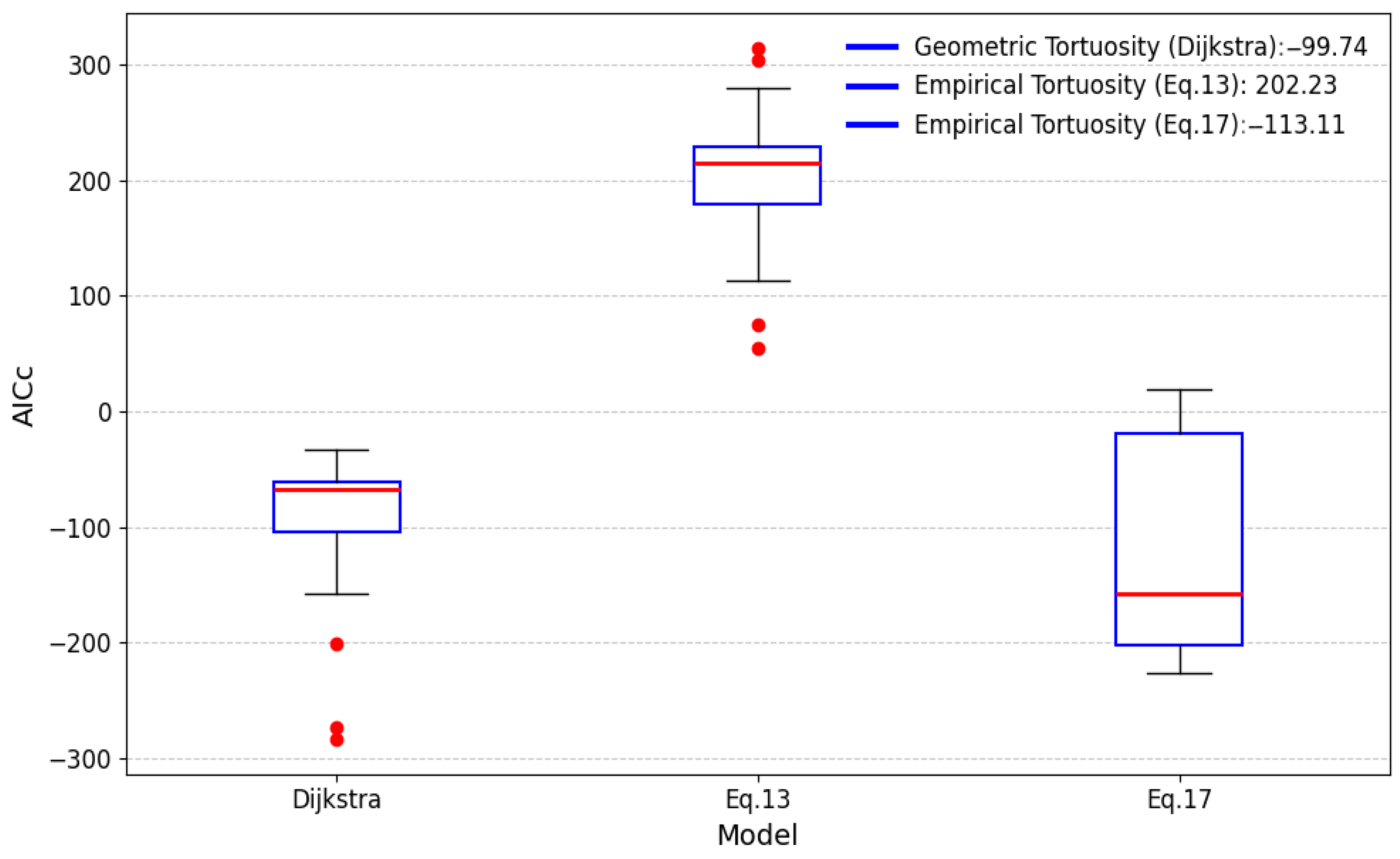
3.9. AICc
A comprehensive comparative analysis was conducted to evaluate three tortuosity estimation models using the AICc as the primary statistical metric. AICc not only assesses the goodness of fit between the model predictions and the reference data but also penalizes model complexity. This balance is critical for preventing overfitting and ensuring that models capture the underlying physical processes in a generalizable and parsimonious manner. Tortuosity values derived from streamline-based calculations, obtained via pore-scale fluid flow simulations, were used as the reference or ground truth to reflect the actual fluid transport pathways through complex pore networks, providing the most physically representative benchmark for model validation.
The boxplot visualization of the relative AICc values for the three models (Figure 16) reveals distinct differences in model performance. The empirical model described by Equation (17) consistently achieves the lowest AICc value (−113.11), indicating the best balance of accuracy and parsimony in representing flow tortuosity. This model’s integration of coordination number and throat length effectively captures key structural and topological features of the pore space, enabling it to approximate flow behavior more closely than the other models.
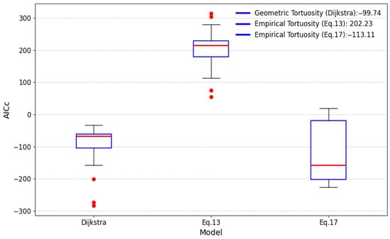
Figure 16.
Boxplots of the AICc distribution.
The Dijkstra model ranks second with an AICc value of 99.74. Despite its purely geometric basis and absence of fitted parameters, it provides a robust estimation of tortuosity by explicitly considering the shortest flow paths within the discretized pore network. Its strength lies in capturing spatial heterogeneity and anisotropy critical for modeling transport phenomena, though it may miss some subtle dynamic flow effects accounted for by the empirical descriptors in Equation (17).
In contrast, the poorly performing Equation (13) had a markedly higher AICc value of 202.23. This model’s sole reliance on porosity, a scalar bulk property, limits its ability to reflect the complex geometry and connectivity inherent in porous media. Consequently, it deviates significantly from the streamline tortuosity reference, emphasizing the insufficiency of bulk porosity alone in capturing transport pathways.
This hierarchy of model performance emphasizes the fundamental principle in porous media transport modeling—that accurate tortuosity prediction must incorporate pore connectivity and topological characteristics rather than relying solely on bulk properties. Geometrically informed and structurally descriptive models outperform simpler empirical relations by more faithfully representing the complex fluid pathways in real rock samples. Additionally, the use of AICc as a quantitative criterion balances model complexity and fit quality, supporting the empirical model of Equation (17) as the most efficient and reliable among those tested.
3.10. Limitations and Perspective
The evaluation of tortuosity across diverse rock types—specifically sandstone and carbonate—demonstrates the crucial influence of pore structure heterogeneity on fluid flow behavior. Carbonate rocks, with their complex and irregular pore geometries, exhibit higher and more variable tortuosity than the relatively homogeneous sandstones. The streamline-based tortuosity from LBM simulations provides the most physically representative results among the four methods assessed. However, the Dijkstra-based geometric and empirical models, particularly Equation (17), offer a practical balance between accuracy and computational efficiency when microstructural parameters are well-integrated.
While an inverse relationship between porosity and tortuosity was consistent, deviations in flow tortuosity highlight the limitations of porosity as a sole predictor of transport behavior. Comparisons with the literature confirm the reliability of the derived values and underline the importance of 3D modeling in capturing realistic flow dynamics. These findings emphasize the need for structure-aware, multi-parametric models for accurate tortuosity estimation in complex porous media, with important implications for reservoir characterization.
This study, while comprehensive in scope, has several limitations that merit consideration. The dataset, although diverse, comprises a fixed number of digital samples comprising ten types of sandstone and carbonate rocks sourced from publicly available micro-CT repositories. While widely used in pore-scale research, these samples may not fully represent the broad variability found in natural formations across different depositional environments or diagenetic histories. Additionally, flow simulations are limited to single-phase, incompressible conditions using the Lattice Boltzmann Method. Realistic reservoir conditions involving multiphase flow, capillary effects, and wettability were not considered, which may restrict the broader applicability of the findings.
The empirical models rely on geometric features, including effective porosity, coordination number, and minimum throat length, derived from image segmentation, which is sensitive to voxel resolution and thresholding. Although the original 10003 voxel datasets were downsampled to 2563 to reduce computational load, the representative elementary volume (REV) condition was maintained to preserve relevant pore-scale features and statistical validity.
In this study, LBM simulations were conducted on 2563 voxel volumes over 30,000 time steps per sample, across 1963 rock samples. All simulations were performed on the RockExplorer supercomputing cluster at the Department of Geophysics, Universitas Padjadjaran, equipped with an Intel® Xeon® Gold 5118 CPU @ 2.30 GHz (48 cores) and 128 GB RAM. The simulations utilized MPI-based parallelization to efficiently distribute computational loads. Each simulation required approximately 1.5 to 2 h of runtime and consumed around 4 to 6 GB of RAM, enabling an average throughput of 10–15 samples per day.
Finally, the assumption of isotropy in tortuosity estimation does not capture directional anisotropy, especially in layered or fractured carbonate rocks. Future studies should consider anisotropic flow, multiphase conditions, and data-driven approaches. Hybrid models that integrate geometric, streamline, and machine learning methods trained on high-resolution, multi-lithology datasets could improve prediction accuracy. Incorporating reactive transport and validating simulations with microfluidic or core flooding experiments would further enhance model robustness and applicability.
4. Conclusions
This study highlights that tortuosity estimation must be lithology-dependent. The empirical model based on Equation (17) provides the best overall agreement with streamline-based tortuosity and is most suitable for sandstones, offering a balance between simplicity and flow-relevance. Dijkstra’s algorithm performs better in carbonates due to its sensitivity to geometric complexity, making it a valuable tool when flow path geometry dominates. In contrast, Equation (13), while computationally simple, is only reliable for high-porosity materials (typically above 50%) and is not recommended for general use. For fast, large-scale screening where moderate accuracy is acceptable, Equation (17) is preferred. Overall, these distinctions help guide the practical application of tortuosity models in different rock types, supporting more informed engineering decisions. The observed weak correlation between porosity and tortuosity is not a limitation but confirms the complex physics of porous media and demonstrates that porosity alone is insufficient to predict fluid flow behavior. Therefore, incorporating additional metrics such as coordination number, throat length, and pore network structure is essential. The analysis of 1963 samples revealed that carbonates exhibit greater heterogeneity compared to sandstones. Future research should focus on hybridizing geometric and streamline approaches, potentially leveraging machine learning to enhance tortuosity prediction accuracy across lithologies.
Author Contributions
B.L.M. and Y.E. conducted the experiments, including sample collection and data acquisition. Sample analysis and data processing were performed by B.L.M. under the guidance of I.A.D. The research concept was developed collaboratively by B.L.M. and I.A.D. B.L.M. was primarily responsible for writing and revising the manuscript. All authors have read and agreed to the published version of the manuscript.
Funding
This research received no external funding.
Institutional Review Board Statement
Not applicable.
Informed Consent Statement
All authors affirm their agreement with this submission. The data included in this manuscript are original and have not been published or submitted for publication in any other venue.
Data Availability Statement
The data that support the study findings are openly available: the raw, filtered, and segmented data of the eleven sandstones at https://doi.org/10.17612/f4h1-w124 and the multi-resolution micro-CT images of sixteen Brazilian pre-salt carbonates at https://www.doi.org/10.17612/xr50-s717 (both accessed on 30 October 2024). The dataset used in this study is available from the corresponding author upon reasonable request.
Acknowledgments
The authors acknowledge the Department of Geophysics, Universitas Padjadjaran, for the supercomputing resources ‘RockExplorer’ made available for conducting the research reported in this paper.
Conflicts of Interest
The authors have no conflicts to disclose.
References
- Akmal, F.; Dzulizar, M.C.; Rafli, M.F.; Az-Zahra, F.; Haq, M.I.K.; Dharmawan, I.A. Machine learning prediction of tortuosity in digital rock. J. Geosci. Eng. Environ. Technol. 2023, 8, 6–12. [Google Scholar] [CrossRef]
- Panini, F.; Ghanbarian, B.; Borello, E.S.; Viberti, D. Estimating geometric tortuosity of saturated rocks from micro-ct images using percolation theory. Transp. Porous Media 2024, 151, 1579–1606. [Google Scholar] [CrossRef]
- Krakowska-Madejska, P. Tortuosity of pore channels in tight rocks as a key parameter in fluid flow ability. Acta Geophys. 2024, 72, 3211–3221. [Google Scholar] [CrossRef]
- Berg, C.F. Permeability description by characteristic length tortuosity, constriction and porosity. Transp. Porous Media 2014, 103, 381–400. [Google Scholar] [CrossRef]
- Yang, S.; Yang, H.; Peng, X.; Lan, X.; Yang, Y.; Zhao, Y.; Zhang, K.; Chen, H. Research of influencing factors on permeability for carbonate rocks based on lbm simulation: A case study of low permeability gas reservoir of Sinian Dengying formation in Sichuan basin. Front. Earth Sci. 2023, 11, 1091431. [Google Scholar] [CrossRef]
- Cheng, Y.; Luo, X.; Zhuo, Q.; Gong, Y.; Liang, L. Description of pore structure of carbonate reservoirs based on fractal dimension. Chem. Process. Syst. 2024, 12, 825. [Google Scholar] [CrossRef]
- Zhang, Y.; Tian, J.; Zhang, X.; Li, J.; Liang, Q.; Zheng, X. Diagenesis evolution and pore types in tight sandstone of Shanxi formation reservoir in Hangjinqi area, ordos basin, northern China. Energies 2022, 15, 470. [Google Scholar] [CrossRef]
- Hu, Y.; Guo, Y.; Qing, H.; Zhang, J. Diagenetic control of reservoir performance and its implications for reservoir prediction in jinci sandstone of upper carboniferous in the middle east ordos basin. ACS Omega 2022, 7, 39697–39717. [Google Scholar] [CrossRef]
- Lin, W.; Chen, L.; Lu, Y.; Hu, H.; Liu, L.; Liu, X.; Wei, W. Diagenesis and its impact on reservoir quality for the Chang 8 oil group tight sandstone of the Yanchang formation (upper Triassic) in southwestern ordos basin, China. J. Petrol. Explor. Prod. Technol. 2017, 7, 947–959. [Google Scholar] [CrossRef]
- Worden, E.H.; Armitage, P.J.; Butcher, A.R.; Churchill, J.M.; Csoma, A.E.; Hollis, C.; Lander, R.H.; Omma, J.E. Petroleum reservoir quality prediction: Overview and contrasting approaches from sandstone and carbonate communities. Geol. Soc. 2018, 435, 1–31. [Google Scholar] [CrossRef]
- Petunin, V.V.; Tutuncu, A.N. Porosity and permeability changes in sandstones and carbonates under stress and their correlation to rock texture. In Proceedings of the SPE Canada Unconventional Resources Conference, Calgary, AB, Canada, 15–17 November 2011. [Google Scholar]
- Azeredo, A.; Duarte, L.; Silva, A. The challenging carbonates from the pre-salt reservoirs offshore Brazil: Facies, palaeoenvironment, and diagenesis. J. S. Am. Earth Sci. 2021, 108, 103202. [Google Scholar] [CrossRef]
- Cataldo, R.; Leite, E.; Rebelo, T.; Mattos, N. Depth-variant pore type modeling in a pre-salt carbonate field offshore Brazil. Front. Earth Sci. 2022, 10, 1014573. [Google Scholar] [CrossRef]
- Pacheco, J.M.; Bayon, P.V.; Correia, U.; Kneller, E.; Peiro, M. Unlocking the properties of a presalt carbonate reservoir offshore Brazil with facies-constrained geostatistical inversion. Lead Edge 2022, 41, 832–839. [Google Scholar] [CrossRef]
- Lima, M.; Pontedeiro, E.; Ramirez, M.; Boyz, A.; Genuchten, M.; Borghi, L.; Couto, P.; Raoof, A. Petrophysical correlations for the permeability of coquinas (carbonate rocks). Transp. Porous Media 2020, 125, 287–308. [Google Scholar] [CrossRef]
- Basso, M.; Belila, A.; Chinelatto, G.; Souza, J.; Vidal, A. Sedimentology and petrophysical analysis of pre-salt lacustrine carbonate reservoir from the santos basin, southeast Brazil. Int. J. Earth Sci. 2021, 110, 2573–2595. [Google Scholar] [CrossRef]
- Moreira, L.; Tedeschi, L.; Silva, A.L.; Santos, R.V.; Vazquez, J.C.; Poley, J.V.; Ros, L.F.D. Deep-burial hydrothermal alteration of the pre-salt carbonate reservoirs from northern Campos basin, offshore Brazil: Evidence from petrography, fluid inclusions, sr, c, and o isotopes. Mar. Pet. Geol. 2020, 113, 104143. [Google Scholar]
- Gomes, J.P. Facies, Diagenesis and Cycles Within the Pre-Salt Deposits from Barra Velha Formation, Santos Basin, Offshore Brazil. Doctoral Thesis, University of Bristol, Bristol, UK, 2021. [Google Scholar]
- Garcia, R.; Mohammadizadeh, S.; Avansi, M.; Basilici, G.; Bomfim, L.; Cunha, O.; Soares, M.; Mesquita, A.; Mahjour, S.; Vidal, A. Geological insights from porosity analysis for sustainable development of santos basin’s presalt carbonate reservoir. Sustainability 2024, 16, 5730. [Google Scholar] [CrossRef]
- Clennell, M.B. Tortuosity: A guide through the maze. Geol. Soc. 1997, 122, 299–344. [Google Scholar] [CrossRef]
- Sun, W.C.; Andrade, J.E.; Rudnicki, J.W. Multiscale method for characterization of porous microstructures and their impact on macroscopic effective permeability. Int. J. Numer. Meth. Engng. 2011, 88, 1260–1279. [Google Scholar] [CrossRef]
- Akmal, F.; Nurcahya, A.; Alexandra, A.; Yulita, I.N.; Kristanto, D.; Dharmawan, I.A. Application of machine learning for estimating the physical parameters of three-dimensional fractures. Appl. Sci. 2024, 14, 12037. [Google Scholar] [CrossRef]
- Az-Zahra, F.; Dharmawan, I.A. A study of geometrical effects on permeability estimation in three-dimensional fractures using the lattice boltzmann method. CFD Lett. 2023, 15, 1–10. [Google Scholar] [CrossRef]
- Alexandra, A.; Akmal, F.; Nurcahya, A.; Yulita, I.N.; Dharmawan, I.A. Estimating two-dimensional physical parameters of digital rocks using deep learning. Phys. Scr. 2025, 100, 016013. [Google Scholar] [CrossRef]
- Santos, J.E.; Trettel, A.; Martinez, M.J. MPLBM-UT: Multiphase LBM library for permeable media analysis. SoftwareX 2022, 18, 101097. [Google Scholar] [CrossRef]
- Nurcahya, A.; Alexandra, A.; Akmal, F.; Dharmawan, I. The lattice boltzmann method and image processing techniques for effective parameter estimation of digital rock. Appl. Sci. 2024, 14, 7509. [Google Scholar] [CrossRef]
- Graczyk, K.M.; Matyka, M. Predicting porosity, permeability, and tortuosity of porous media from images by deep learning. Sci. Rep. 2020, 10, 21488. [Google Scholar] [CrossRef] [PubMed]
- Matyka, M.; Khalili, A.; Koza, Z. Tortuosity-porosity relation in porous media flow. Phys. Rev. E 2008, 78, 026306. [Google Scholar] [CrossRef]
- Haq, M.I.K.; Yulita, I.N.; A Dharmawan, I. A study of transfer learning in digital rock properties measurement. Mach. Learn. Sci. Technol. 2023, 4, 035034. [Google Scholar] [CrossRef]
- Avila, J.; Pagalo, J.; Espinoza-Andaluz, A. Evaluation of geometric tortuosity for 3d digitally generated porous media considering the pore size distribution and the a-star algorithm. Sci. Rep. 2022, 12, 19463. [Google Scholar] [CrossRef]
- Ghanbarian, B.; Esmaeilpour, M.; Ziff, R.M.; Sashimi, M. Effect of pore-scale heterogeneity on scale-dependent permeability: Pore-network simulation and finite-size scaling analysis. Water Resour. 2021, 57, e2021WR030664. [Google Scholar] [CrossRef]
- Bernabe, Y.; Li, M.; Maineult, A. Permeability and pore connectivity: A new model based on network simulations. J. Geophys. Res. Solid Earth 2010, 115, B10203. [Google Scholar] [CrossRef]
- Nurcahya, A.; Dharmawan, I.A. Enhanced understanding of fluid flow and effective properties in three dimensional porous rock using lattice boltzmann simulation and image-based correlation studies. Phys. Fluids 2025, 37, 053607. [Google Scholar] [CrossRef]
- Bini, F.; Pica, A.; Novelli, S.; Pecci, R. 3D FEM model to simulate Brownian motion inside trabecular tissue from human femoral head. Comput. Methods Biomech. Biomed. Eng. Imaging Vis. 2021, 10, 500–507. [Google Scholar] [CrossRef]
- Vidal, A.; Menezes dos Anjos, C.E.; Medeiros, L.; Surmas, R.; Neta, A.; Evsukoff, A.; Vargas, J. 16 Brazilian Pre-Salt Carbonates: Multi-Resolution Micro-ct Images; Digital Rocks Portal: Austin, TX, USA, 2025. [Google Scholar]
- Neumann, R.; Andreeta, M.; Lucas-Oliveira, E. 11 Sandstones: Raw, Filtered and Segmented Data; Digital Rocks Portal: Austin, TX, USA, 2025. [Google Scholar]
- Ashirbekov, A.; Kabdenova, B.; Monaco, E.; Rojas-Solorzano, L.R. Equation of states crossover enhancement of pseudopotential lattice boltzmann modelling of CO2 flow in homogeneous porous media. Fluids 2021, 6, 434. [Google Scholar] [CrossRef]
- Yu, Y.; Qin, Z.; Chen, S.; Shu, S.; Yuan, H.-Z. Two-relaxation-time regularized lattice boltzmann model for navier-stokes equations. arXiv 2023, arXiv:2312.10318. [Google Scholar]
- Yu, Y.; Qin, Z.; Yuan, H.; Shu, S. Two-relaxation-time regularized lattice boltzmann model for convection-diffusion equation with spatially dependent coefficients. Appl. Math. Comput. 2025, 488, 129135. [Google Scholar] [CrossRef]
- Cecen, A.; Wargo, E.; Hanna, A.; Turner, D.; Kalidiudi, S.; Kumbur, E. 3-d microstructure analysis of fuel cell materials: Spatial distributions of tortuosity, void size and diffusivity. J. Electrochem. Soc. 2012, 159, B299–B307. [Google Scholar] [CrossRef]
- Ghanbarian, B.; Hunt, A.G.; Sashimi, M.; Ewing, R.P.; Skinner, T.E. Percolation theory generates a physically based description of tortuosity in saturated and unsaturated porous media. Soil Sci. Soc. Am. J. 2013, 77, 1920–1929. [Google Scholar] [CrossRef]
- Akaike, H. A new look at statistical model identification. IEEE Trans. Autom. Control 1974, AC-19, 716–723. [Google Scholar] [CrossRef]
- Hurvich, C.M.; Tsai, C. Regression and time series model selection in small samples. Biometrika 1989, 76, 297–307. [Google Scholar] [CrossRef]
- Ghanbarian, B.; Lin, W.; Pires, L.F. Scale dependence of tortuosity in soils under contrasting cultivation conditions. Soil Tillage Res. 2023, 233, 105788. [Google Scholar] [CrossRef]
- Koponen, A.; Kataja, M.; Timonen, J.; Kandhai, D. Simulations of single-fluid flow in porous media. Int. J. Mod. Phys. C 1998, 9, 1505–1521. [Google Scholar] [CrossRef]


Disclaimer/Publisher’s Note: The statements, opinions and data contained in all publications are solely those of the individual author(s) and contributor(s) and not of MDPI and/or the editor(s). MDPI and/or the editor(s) disclaim responsibility for any injury to people or property resulting from any ideas, methods, instructions or products referred to in the content. |
© 2025 by the authors. Licensee MDPI, Basel, Switzerland. This article is an open access article distributed under the terms and conditions of the Creative Commons Attribution (CC BY) license (https://creativecommons.org/licenses/by/4.0/).