A LiDAR-Driven Approach for Crop Row Detection and Navigation Line Extraction in Soybean–Maize Intercropping Systems

Abstract

Crop row identification and navigation line extraction are essential components for enabling autonomous operations of agricultural machinery. Aiming at the soybean–maize strip intercropping system, this study proposes a LiDAR-based algorithm for crop row detection and navigation line extraction. The proposed method consists of four primary stages: point cloud preprocessing, crop row region identification, feature point clustering, and navigation line extraction. Specifically, a combination of K-means and Euclidean clustering algorithms is employed to extract feature points representing crop rows. The central lines of the crop rows are then fitted using the least squares method, and a stable navigation path is constructed based on angle bisector principles. Field experiments were conducted under three representative scenarios: broken rows with missing plants, low occlusion, and high occlusion. The results demonstrate that the proposed method exhibits strong adaptability and robustness across various environments, achieving over 80% accuracy in navigation line extraction, with up to 90% in low-occlusion settings. The average navigation angle was controlled within 0.28°, with the minimum reaching 0.17°, and the average processing time remained below 75.62 ms. Moreover, lateral deviation tests confirmed the method’s high precision and consistency in path tracking, validating its feasibility and practicality for application in strip intercropping systems.

1. Introduction

Soybean and maize are two of the most important staple and oilseed crops in China. The strip intercropping of soybean and maize has been widely adopted across the country, offering a mutually beneficial growth environment by leveraging the edge-row advantages of maize [1,2,3,4]. However, current machinery operations in soybean–maize strip intercropping systems still largely depend on manual intervention, often resulting in issues such as seedling damage caused by wheel traffic. To address these challenges, enabling autonomous operation of agricultural machinery has become a research focus [5,6]. In strip intercropping systems, soybean and maize are typically sown in rows using precision seeding techniques, which makes it feasible to plan inter-row wheel paths by extracting the central lines of the crop rows. At present, two primary approaches are used for crop row identification and navigation line extraction: machine vision and LiDAR-based techniques.

Research on crop row detection and navigation line extraction began relatively early in foreign countries. Many studies have employed machine vision and deep learning models to identify crop rows and extract navigation paths [7,8,9,10,11]. For example, Kise et al. [12] utilized binocular vision techniques to detect soybean crop rows by integrating multiple image processing algorithms. However, the performance of their approach requires further validation in complex environments with dense weeds or heavy shadows. Diao et al. [13] proposed an improved UNet-based model for detecting the central lines of maize crop rows. Their method achieved promising results, significantly reducing both the average fitting time and angular error compared to traditional vertical projection methods, reaching 66 ms and 4.37°, respectively. Similarly, Lin et al. [14] applied a convolutional neural network (CNN) to detect rice seedlings and accurately determine inter-row spacing in paddy fields.

However, machine vision techniques still face numerous challenges in complex and variable field environments. Factors such as shadows, fluctuating lighting conditions, and lengthy image processing times can adversely affect the accuracy of crop row detection and navigation line extraction. To address these issues, Shi et al. [15] employed an improved YOLOv8 model for the detection of multiple crop types. The experimental results demonstrated the model’s exceptional performance, with mean average precision (mAP) values consistently exceeding 96.4%, highlighting its robustness and stability in diverse agricultural scenarios.

Although machine vision and deep learning techniques have achieved significant progress in capturing crop image features, the variability of field environments and differences in agronomic traits pose substantial challenges to image processing. The complexity of field conditions often introduces large amounts of redundant information into the captured images, which not only increases the computational burden and prolongs processing time but also complicates stereo matching. These factors collectively degrade the accuracy of crop row detection and navigation line extraction [16,17].

In contrast, LiDAR technology determines the distance to a target by emitting laser pulses, enabling the direct acquisition of spatial information [18,19,20]. Moreover, LiDAR is inherently robust to variations in shadow and lighting conditions [21,22], which gives it a significant advantage in complex and highly occluded environments. With continuous technological advancements and declining hardware costs, LiDAR is becoming increasingly promising for agricultural applications. In recent years, both domestic and international researchers have made notable progress in applying LiDAR to crop row detection. For instance, Barawid et al. [23] successfully integrated two-dimensional LiDAR with the Hough transform algorithm to achieve accurate navigation of autonomous vehicles in real-world environments, such as orchards. Similarly, Malavazi et al. [24] improved the PEARL method to detect crop row centerlines and generate navigation paths in weeding operations under poor GPS signal conditions, thereby enhancing operational efficiency.

LiDAR technology has also demonstrated remarkable effectiveness in field-based crop recognition. Bergerman et al. [25] and Zhang et al. [26] conducted in-depth studies on autonomous navigation and crop row centerline detection in maize fields. By applying threshold-based filtering methods, they accurately extracted crop row feature points and efficiently derived the centerlines using the least squares method. The experimental results showed that the centerline extraction rates for maize crop rows reached 95.1% and 87.3%, respectively, with both the accuracy and processing speed outperforming those of traditional machine vision-based approaches.

In summary, although LiDAR technology has achieved significant progress in crop row detection, most existing studies have focused on single-crop systems or regular planting patterns. Research remains limited for more complex configurations, such as the soybean–maize strip intercropping system characterized by spatial heterogeneity and irregular canopy distribution. To address this gap, this study proposes a LiDAR-based algorithm for crop row detection and navigation line extraction tailored to intercropping systems. The algorithm is evaluated using navigation angle, lateral deviation, and processing time as performance metrics. Field experiments under three representative scenarios—broken rows with missing plants, low occlusion, and high occlusion—were conducted to assess its adaptability and robustness. This work aims to enable accurate crop row identification and stable navigation path generation in structurally complex fields, providing a reliable technical foundation for intelligent and autonomous agricultural operations.

2. Materials and Methods

2.1. Experimental Data Collection and Processing

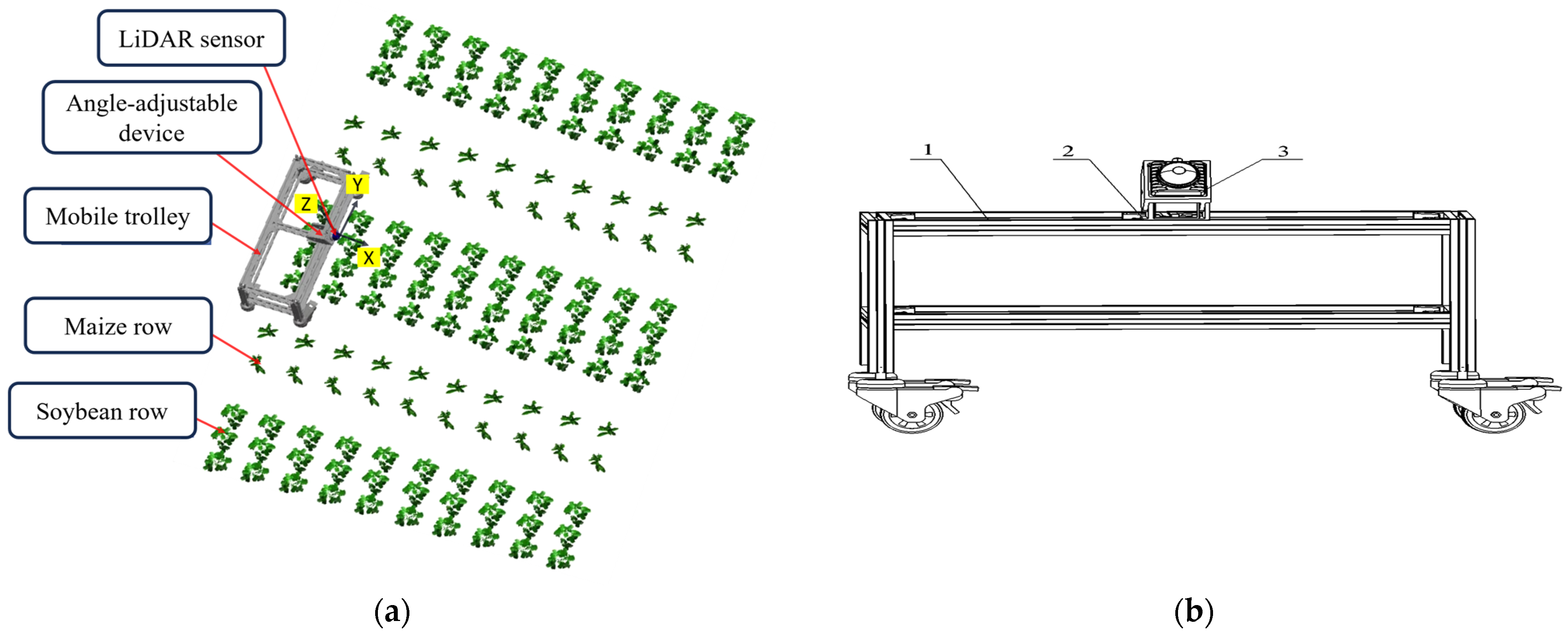
2.1.1. Field Point Cloud Data Collection

The data used in this study were collected at a soybean–maize strip intercropping experimental site located in Biancheng Town, Jurong City, Jiangsu Province, China. The point cloud data were obtained using a self-developed data acquisition platform, which primarily consisted of a mobile trolley, a MID-360 3D LiDAR sensor, an adjustable mounting bracket, and an upper computer control system, as illustrated in Figure 1.

During the data collection process, the mobile trolley moved steadily along the inter-row paths, while the LiDAR system continuously scanned the field in real time, capturing the three-dimensional spatial information of the crops.

The MID-360 LiDAR sensor(Livox Technology, Shenzhen, China) features a high-density scanning capacity of 240,000 points per second with a 360° horizontal and 59° vertical field of view and a detection range of 0.1 to 100 m. This enables a comprehensive perception of complex agricultural field environments. The upper computer was responsible for configuring LiDAR parameters and managing data synchronization, ensuring the stability and continuity of point cloud acquisition. This setup provided high-quality data support for subsequent crop row detection and navigation modeling.

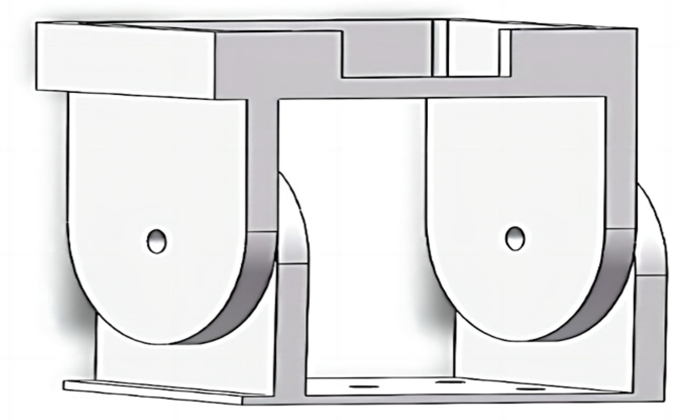
2.1.2. Key Component Design

To accommodate variations in crop height and complex terrain conditions, a compact and efficient LiDAR angle adjustment device was designed and integrated in this study. The structural layout of the device is shown in Figure 2. Specifically tailored for LiDAR installation, the device features a base measuring 80 mm × 80 mm × 20 mm, offering excellent adaptability for mounting and high structural stability. This ensures smooth operation of the LiDAR and maintains data accuracy during field deployment. The overall dimensions of the device are 80 mm × 80 mm × 126 mm, allowing for seamless integration with the mobile platform in space-constrained environments.

To enhance the mechanical stability and data acquisition reliability of the device under varying operational conditions, multiple sets of positioning holes were incorporated into the design. These features ensure secure mounting on the mobile platform, thereby improving the overall durability and operational safety of the system. In addition, the angle adjustment mechanism adopts a manually operated hinged design, enabling flexible pitch adjustments of the LiDAR sensor within a range of 0° to 180°. This provides robust mechanical support for multi-angle 3D perception in complex field environments.

2.2. Crop Row Recognition and Navigation Line Extraction

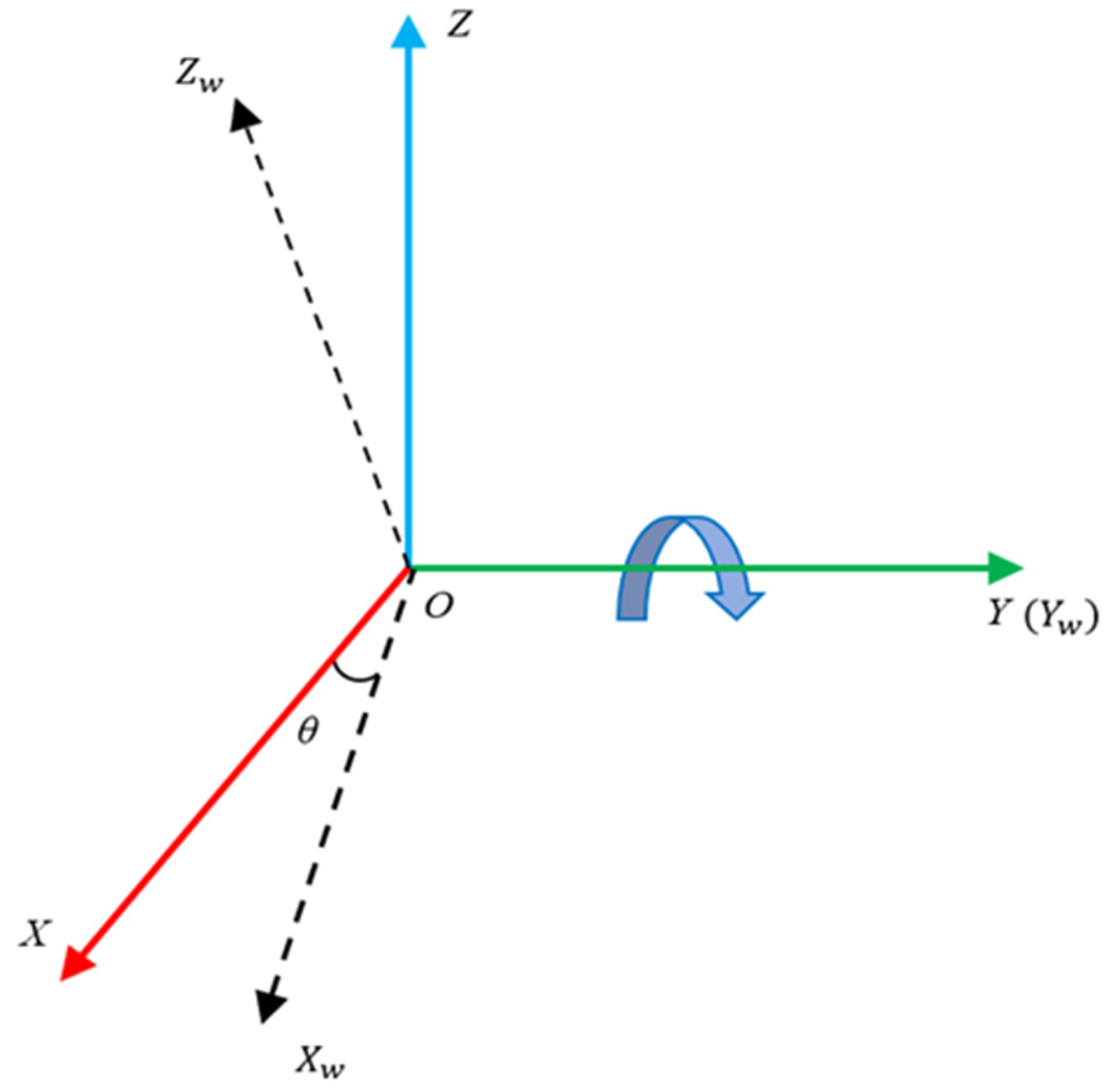
2.2.1. Point Cloud Filtering and Coordinate Transformation

Due to the influence of environmental factors, LiDAR hardware, and the physical characteristics of scanned objects, the acquired point cloud data inevitably contain noise. These noisy points not only increase the data volume but also reduce the accuracy of object recognition and feature extraction. Therefore, this study employs the Kalman filtering algorithm to process the raw point cloud data. The Kalman filter is computed using the following formulation:

$${\widehat{x}}_{k|k-1}=A{\widehat{x}}_{k-1|k-1}+B{u}_k$$

(1)

$$P_{k|k-1}=A{P}_{k-1|k-1}{A}^T+Q$$

(2)

$${\widehat{x}}_{k|k}={\widehat{x}}_{k|k-1}+K_k(z_k-H{\widehat{x}}_{k|k-1})$$

(3)

$$K_k=P_{k|k-1}{H}^T{(H{P}_{k|k-1}{H}^T+R)}^{-1}$$

(4)

In the equation, P represents the error covariance matrix; A, B, and H denote the state transition matrix, control matrix, and observation matrix, respectively; Q and R correspond to the process noise and observation noise covariance matrices; and K_k is the Kalman gain.

In this study, the 3D spatial coordinates of each point in the LiDAR point cloud are modeled and updated as the state variables in the Kalman filter, enabling dynamic optimization of position fluctuations. After filtering, high-frequency noise is effectively suppressed, and the continuity between adjacent points is significantly enhanced. As shown in Figure 3, the filtered point cloud provides a reliable and structured data foundation for subsequent crop row recognition and modeling.

To ensure coordinate consistency, a coordinate transformation was performed on the crop point cloud data, converting the LiDAR-based coordinates into the global (world) coordinate system, as illustrated in Figure 4. The original XYZ coordinate system is defined by the LiDAR sensor, which changes dynamically with the movement and tilt of the mobile platform. After transformation, the point cloud data are aligned with the fixed global coordinate axes (X_w, Y_w, Z_w), ensuring spatial consistency and accuracy throughout the analysis.

To transform the point cloud data from the LiDAR coordinate system to the world coordinate system, the overall rotation matrix of the LiDAR frame, denoted as R, is defined. The calculation of R is given by the following equation:

$$R=R_x\left(\alpha \right)·R_y\left(\beta \right)·R_z\left(\gamma \right)$$

(5)

In the equation, α, β, and γ represent the rotation angles of the LiDAR point cloud around the X, Y, and Z axes, respectively.

The simplified rotation matrix is then expressed as follows:

$$R_Y\left(\theta \right)=\left[\begin{array}{ccc}\cos \theta & 0& \sin \theta \\ 0& 1& 0\\ -\sin \theta & 0& \cos \theta \end{array}\right]$$

(6)

Furthermore, the coordinate transformation matrix was applied to convert the point cloud data from the LiDAR coordinate system to the world coordinate system. The transformation is performed according to the following equation:

$$\left[\begin{array}{c}x\\ y\\ z\end{array}\right]=R_y(\theta )$$

(7)

In the equation, θ denotes the LiDAR tilt angle (in degrees); x′, y′, and z′ represent the coordinates of the point cloud in the LiDAR coordinate system; and x, y, and z correspond to the transformed coordinates in the world coordinate system.

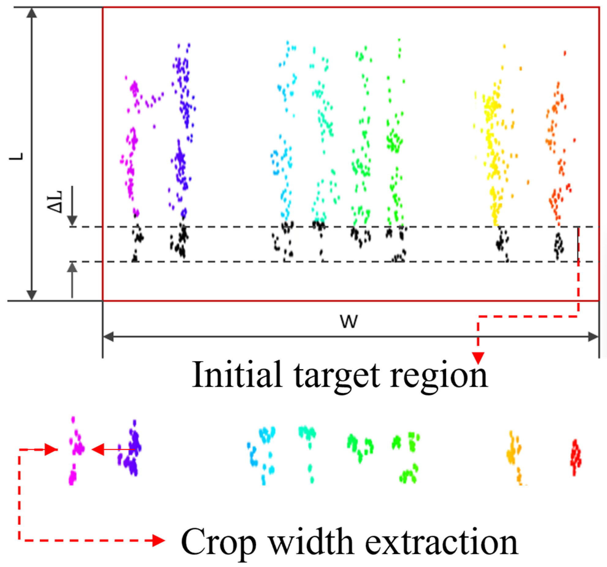
2.2.2. Determination of the Crop Row Target Region

To effectively extract the crop row region, the initial horizontal target area was defined based on the plant spacing characteristics of soybean and maize. The width

W of the target area was set to 3.5 m, and the length ΔL was set to 0.20 m. This initial area served as the analysis range for point cloud projection, providing support for estimating the row-wise crop width.

Within the initial target region, a K-means clustering algorithm was applied to the projected point cloud data to estimate the crop width. Based on the clustering results, the distribution width of each cluster was statistically analyzed, and the maximum width was selected as the basis for subsequent region delineation, as illustrated in Figure 5.

After the crop row point cloud data were framed, as shown in Figure 6, a Euclidean clustering algorithm was employed to further segment and refine the soybean and maize row structures. By calculating the centroid coordinates of each cluster and incorporating the inter-row spacing characteristics, the algorithm effectively distinguished between soybean and maize rows.

Euclidean distance is a fundamental spatial metric used to measure the straight-line distance between two points in three-dimensional space. The calculation formula is as follows:

$$d=\sqrt{{(x_2-x_1)}^2+{(y_2-y_1)}^2+{(z_2-z_1)}^2}$$

(8)

In the equation, (x₁, y₁, z₁) and (x₂, y₂, z₂) represent the 3D coordinates of two points within the feature crop row point cloud data.

To control the clustering merging process, a distance threshold, thresh Dthresh, was defined. This threshold was determined based on the maximum crop width extracted from the initial target region. During the clustering procedure, a union-find (disjoint-set) structure was employed to determine whether two clusters should be merged: if the Euclidean distance between two clusters was less than or equal to thresh Dthresh, they were merged into the same category. This strategy enabled further refinement and accurate separation of the soybean and maize row regions, as illustrated in Figure 7.

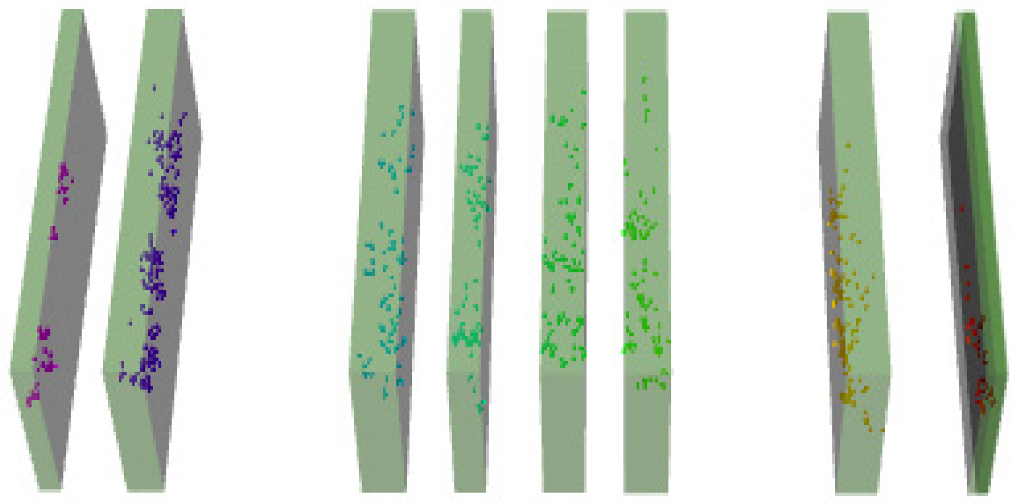
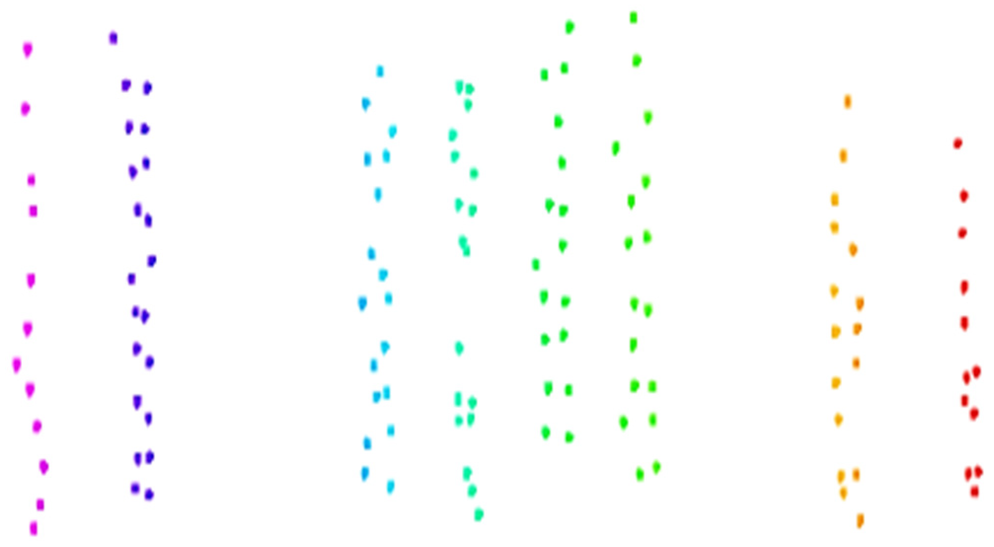
2.2.3. Crop Row Centerline Fitting

To accurately identify soybean and maize rows within the main crop regions and enable path guidance, this study proposes a least-squares-based centerline fitting method. This approach is used to extract the centerline of each crop row and subsequently generate a navigation line. The core objective of the method is to minimize the error between the point cloud data and the fitted curve, thereby producing an optimal linear model that reflects the structural characteristics of the crop rows. The corresponding coordinate system is illustrated in Figure 7.

Given the linear distribution characteristics of crop rows in the soybean–maize strip intercropping system, a linear function was selected to fit the point cloud data of the main crop row regions. The fitting model is expressed as follows:

$$y=Ax+B$$

(9)

In the equation, y and x represent the coordinates of the points along the Y_w-axis and X_w-axis, respectively. k and b are the model parameters to be estimated, corresponding to the slope and intercept of the fitted line, respectively.

Based on the proposed model, the centerlines of soybean and maize rows were extracted by fitting the point cloud data within their respective main stem regions. As shown in Figure 8, the colored points represent valid point cloud data within the crop row region, and the fitted lines denote the extracted crop centerlines. The results indicate that the fitted lines accurately passed through the core point clusters, reflecting the actual distribution patterns of the rows and providing a reliable basis for subsequent path planning and navigation control.

To quantitatively assess the fitting performance, we employed the coefficient of determination (R²) and root mean square error (RMSE) as evaluation metrics. The experimental results showed an average R² value of 0.973 and an average RMSE of 0.023 m, indicating high fitting accuracy and robustness.

2.2.4. Crop Row Navigation Line Extraction

To enable autonomous navigation of agricultural robots between intercropped crop rows, a navigation path extraction method based on the angle bisector principle was proposed. Geometrically, the bisector ensures an evenly balanced orientation between adjacent crop rows, reducing abrupt directional changes and improving the smoothness and stability of the navigation path. This method integrates the centerline information from both the left and right sides of soybean and maize rows to generate a stable and guidance-effective navigation path.

First, the centerlines of the crop rows on both sides of the mobile platform’s operating direction are extracted. For the soybean rows, the average slope of the left and right centerlines is calculated to construct a navigation line Y₁, expressed as y₁ = k₁x₁ + b₁. Similarly, for the maize rows, the average slope of the left and right centerlines is calculated to construct another navigation line Y₂, given by y₂ = k₂x₂ + b₂.

To further generate a unified navigation path, the intersection point (x₀, y₀) between Y₁ and Y₂ must be calculated. The computation is as follows:

$$\left\{\begin{array}{c}{x}_0={\displaystyle \frac{b_2-b_1}{k_1-k_2}}\\ y_0=k_1{x}_0+b_1\end{array}\right.$$

(10)

The slope of the average navigation line, denoted as m₀, is calculated based on the slopes of the navigation lines corresponding to the soybean and maize crop rows. The calculation formula is as follows:

$$m_0={\displaystyle \frac{k_1+k_2}{2}}$$

(11)

Finally, using the intersection point (x₀, y₀) as a reference point and combining it with the average slope m₀, the final navigation path Y_avg is determined using the point-slope form. The expression is as follows:

$$y-y_0=m_0(x-x_0)$$

(12)

The results of navigation line extraction are shown in Figure 9, where the green lines represent the fitted centerlines of the soybean and maize crop rows and the red line indicates the extracted navigation path.

3. Results and Discussion

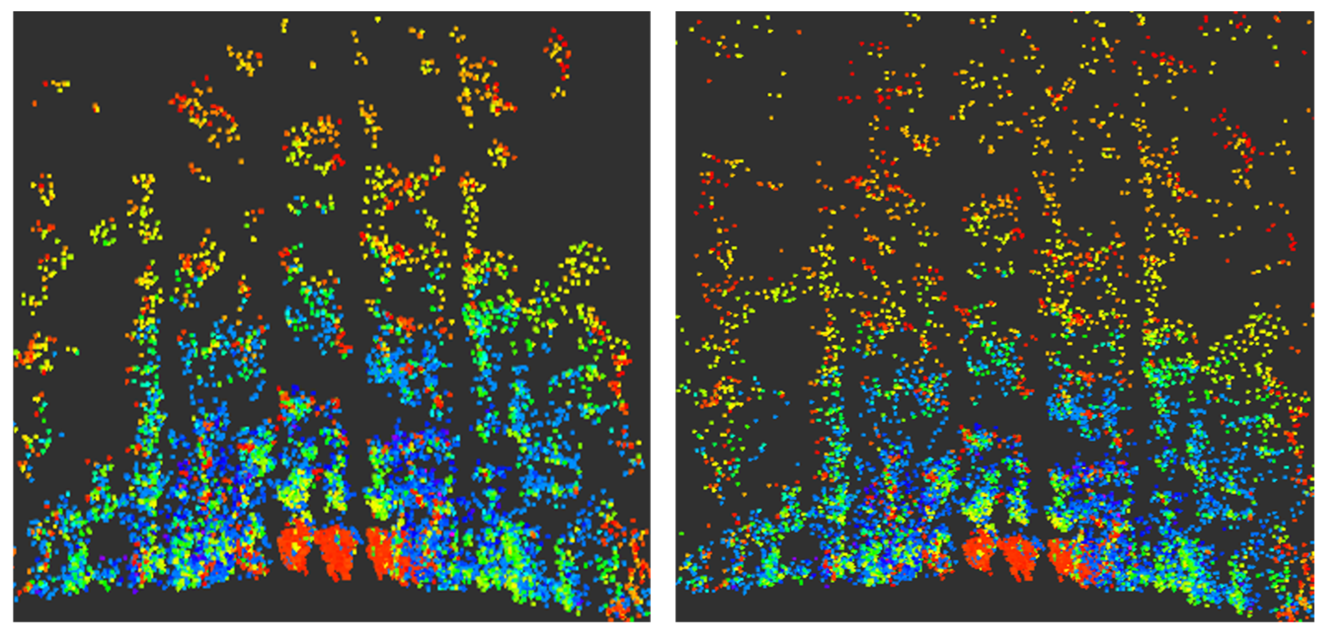
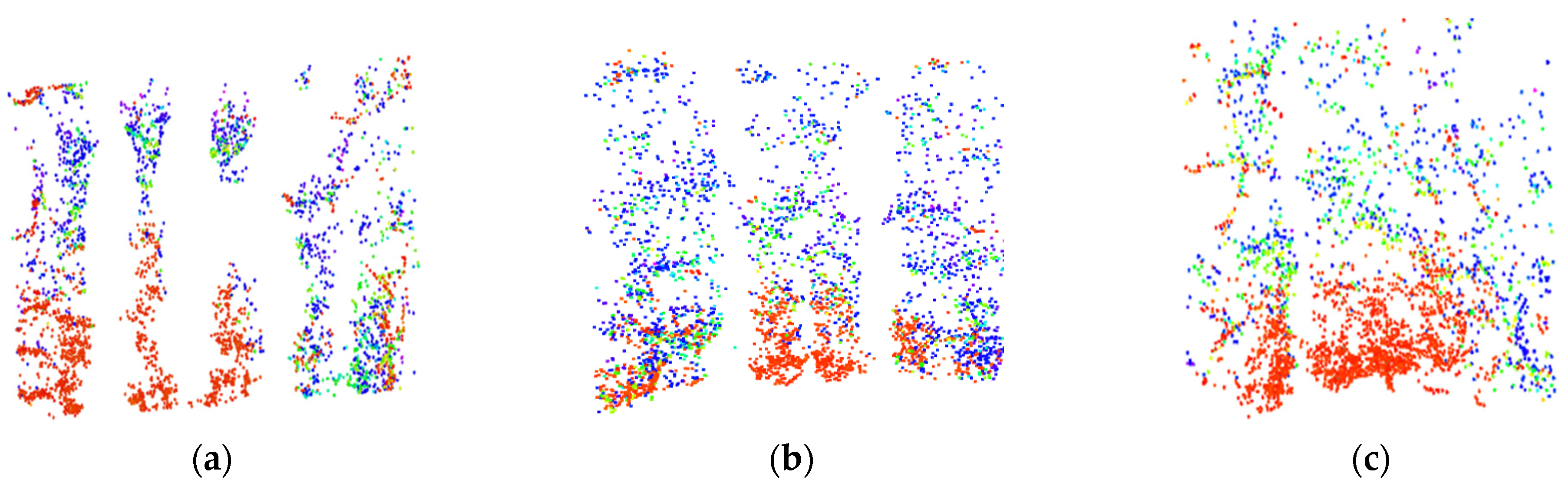
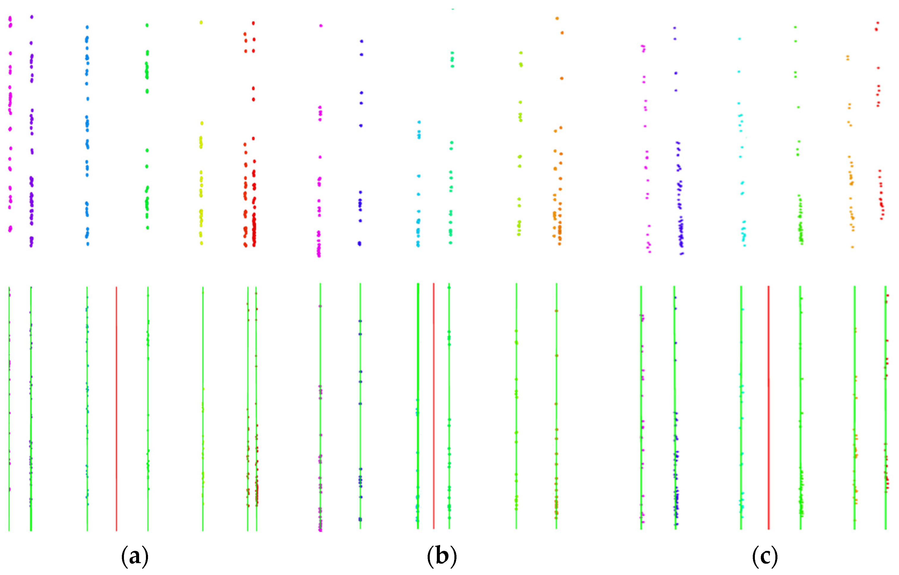
3.1. Crop Row Detection and Navigation Line Extraction

To evaluate the adaptability of the proposed crop row detection and navigation line extraction algorithm under different field conditions, point cloud processing and analysis were conducted in three typical scenarios. The results are presented in Figure 10. All experiments were conducted on a workstation running the Windows 11 operating system equipped with an Intel Core i7-14700F processor and an NVIDIA GeForce RTX 4060 Ti graphics card (Lenovo, Beijing, China).

Figure 10a shows the point cloud data of soybean and maize crop rows under a broken-row and missing-plant condition, labeled scenario S1. Apparent discontinuities in the crop rows can be observed, reflecting the challenging conditions of this test case. Figure 10b corresponds to a low-occlusion scenario, labeled S2, where the crop row structures are clearly defined, facilitating accurate navigation path extraction. Figure 10c illustrates a high-occlusion scenario, in which the ground surface is almost entirely covered by soybean foliage, significantly increasing the difficulty of crop row detection and path planning.

In this study, the accuracy of crop row detection and navigation line extraction under actual field operating conditions was experimentally validated. To ensure that agricultural machinery can accurately navigate along crop rows during field operations, 100 frames of point cloud data were randomly selected from each test scenario for processing and analysis. The average extraction accuracy of the navigation lines in each frame was calculated using Equation (10). The experimental results are presented in Figure 11 and

Table 1. Navigation line extraction results.

Test Scenario	Average Soybean Plant Height/cm		Average Maize Plant Height/cm		Average Accuracy/%
	Tested Value	Actual Value	Tested Value	Actual Value
S1	10	14.86	20	22.67	81
S2	30	31.71	50	45.14	90
S3	40	44.94	75	77.69	84

.

$$\theta =arctan\left(m_0\right)$$

(13)

In the equation, the navigation angle θ represents the angle between the forward direction of the agricultural machinery and the extracted navigation line.

Table 1 presents the navigation line extraction results under different field scenarios. The proposed method achieved robust performance in all three conditions, with accuracies above 80%. Scenario S2 (low occlusion) yielded the highest accuracy (90%) due to uniform crop distribution and clearly distinguishable ground features, which enabled more effective point cloud segmentation and line extraction.

In contrast, scenario S1 exhibited reduced accuracy (81%) caused by discontinuous crop rows and uneven point cloud density. Scenario S3 faced the most significant occlusion from soybean leaves, leading to partial ground-level data loss and a moderate accuracy of 84%. These results underscore the challenges of high-occlusion environments, where poor visibility and structural overlap can compromise vision-based navigation accuracy.

3.2. Effect of the Filtering Algorithm on Navigation Angle Under Multiple Scenarios

To evaluate the effectiveness of the filtering algorithm in optimizing the navigation angle during operation, this study conducted a comparative experiment using 100 randomly selected frames of point cloud data. The data were processed with and without the filtering algorithm, and the results were compared. The average navigation angle and average processing time were used as evaluation metrics to assess the impact of the filtering algorithm on navigation accuracy.

Figure 12 compares the variation trends of the navigation angle before and after filtering. The black curve represents the raw data with evident high-frequency fluctuations, while the red curve shows a smoother trend after applying the filtering algorithm. Quantitative analysis shows that the angle variance decreased from 0.128°² to 0.056°², representing a 56.3% reduction. This demonstrates that the filtering algorithm effectively suppresses instantaneous noise and abrupt deviations, significantly improving the stability and continuity of the navigation signal. Such enhancement provides more reliable support for the smooth operation of agricultural machinery in dynamic field environments.

Table 2. Average navigation angle during the homework process in different scenarios.

Test Scenario	Average Navigation Angle/°	Average Processing Time ± SD/ms
S1	0.28	42.36 (±20.56)
S2	0.17	46.96 (±19.38)
S3	0.18	75.62 (±21.70)

summarizes the average navigation angle and processing time under different field conditions. The results indicate that the variation in the average navigation angle across the three operational scenarios is minimal, ranging from 0.17° to 0.28°. This suggests that the extracted navigation paths are directionally stable, with good linear consistency and continuity, minimizing the risk of significant deviations. Such stability provides a solid foundation for the reliable navigation of agricultural equipment.

However, the average processing time varied considerably across different scenarios. In the low-occlusion (S2) and broken-row (S1) conditions, the average processing times were 46.96 ms and 42.36 ms, respectively, indicating high computational efficiency. In contrast, under the high-occlusion condition (S3), the average processing time increased to 75.62 ms, suggesting that the system requires more computational resources to complete crop row segmentation and centerline extraction when facing significant plant occlusion and point cloud noise. These results reveal that occlusion not only affects recognition accuracy but also poses challenges to the system’s real-time performance.

In summary, although the navigation angle remained relatively stable across different scenarios, processing efficiency was strongly influenced by environmental complexity. Therefore, enhancing the efficiency of point cloud preprocessing algorithms or incorporating structural optimization strategies will be key to improving overall system performance in high-occlusion environments.

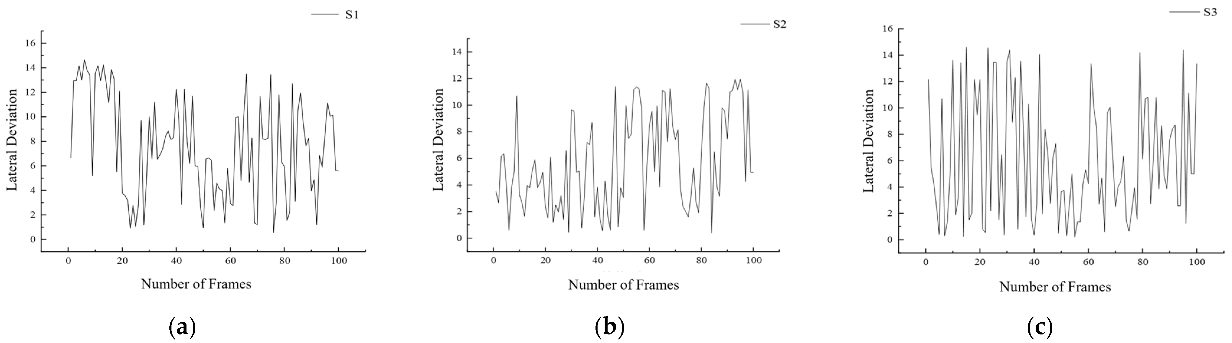
3.3. Influence of Multi-Scenario Conditions on the Navigation Line Extraction Algorithm

To further validate the reliability and robustness of the proposed navigation line extraction algorithm under multiple scenarios, Equation (14) was used to calculate the lateral deviation during the navigation process. Corresponding deviation curves were plotted to visualize the navigation performance in different conditions, including broken-row and missing-plant scenarios, low-occlusion scenarios, and high-occlusion scenarios.

$$d={\displaystyle \frac{\left|m_0{x}_0+y_0+(y_2-m_0{x}_2)\right|}{\sqrt{m_0^2+1}}}$$

(14)

As shown in the data in Figure 13, the maximum lateral deviation under the low-occlusion scenario (S2) was the smallest, reaching only 11.95 cm. However, the minimum and average lateral deviations were relatively larger, at 0.40 cm and 5.76 cm, respectively, indicating that the S2 scenario effectively reduced the influence of external factors, resulting in more concentrated and stable data. In contrast, although the overall average deviations in the broken-row (S1) and high-occlusion (S3) scenarios were slightly higher, the data exhibited relatively stable trends.

Table 3. Lateral deviation in the process of motion in different scenarios.

Test Scenario	Maximum Lateral Deviation/cm	Minimum Lateral Deviation/cm	Average Lateral Deviation/cm	Standard Deviation/cm
S1	14.65	0.55	7.55	4.07
S2	11.95	0.40	5.76	3.56
S3	14.60	0.20	6.34	4.66

presents the lateral deviation performance of the system under different levels of field occlusion. The results show that the average lateral deviation in the S2 (low-occlusion) scenario was 5.76 cm, which is significantly lower than the 7.55 cm observed in the S1 (broken-row) scenario, with a difference of 1.79 cm. The S3 (high-occlusion) scenario also showed a lower average deviation of 6.34 cm, 1.21 cm less than that of S1.

This trend suggests that, compared to the path discontinuity caused by structural breaks and missing plants, the perceptual interference introduced by occlusion has a milder impact on system navigation control. Broken rows interrupt the continuity of the crop structure, making path prediction more difficult and leading to greater deviations. In contrast, although the high-occlusion environment involves significant leaf coverage, the spatial distribution of the crops remains coherent, allowing the system to rely on residual structural features for effective detection and navigation correction.

Moreover, the maximum deviation (11.95 cm) and standard deviation (3.56 cm) in the S2 scenario were also lower than those in S1 and S3, further confirming the advantage of low-occlusion environments in improving path stability. While the S3 scenario exhibited a slightly larger deviation range, the system maintained an acceptable average error level even in complex point cloud conditions, demonstrating strong robustness.

In summary, the experimental results confirm that the proposed navigation system can maintain high path accuracy and operational stability under various crop morphologies and occlusion conditions. The system performed especially well under low-occlusion environments, validating the accuracy and environmental adaptability of the proposed crop row detection and navigation line extraction algorithm. These findings provide both theoretical and data support for the precise navigation of agricultural machinery in strip intercropping systems.

4. Conclusions

This study proposes a LiDAR-based method for crop row detection and navigation line extraction tailored to soybean–maize strip intercropping systems. The method consists of four main steps: point cloud preprocessing, crop row identification, feature point clustering, and navigation line extraction. The experimental results demonstrate that the proposed approach effectively identifies crop rows and extracts navigation paths under various field conditions.

Under the low-occlusion condition (S2), the system achieved superior performance, with a crop row detection accuracy of 90%, an average navigation angle deviation of 0.17°, and a processing time of 46.96 ms—demonstrating both high precision and real-time efficiency. In the broken-row and missing-plant scenario (S1), detection accuracy declined to 81% due to disrupted row continuity. Despite significant leaf occlusion in scenario S3, the system maintained an accuracy of 84%, highlighting its resilience under visually complex conditions. Lateral deviation tests further substantiated the system’s reliability. In S2, the average deviation was 5.76 cm, with a maximum of 11.95 cm; although deviations increased in S1 and S3, they remained within acceptable operational thresholds. Collectively, these results confirm the method’s robustness and adaptability across diverse and challenging field scenarios.

In summary, the proposed crop row detection and navigation line extraction algorithm enables accurate path planning for soybean–maize strip intercropping systems. Although performance varied slightly under complex field conditions, the system exhibited strong adaptability and robustness. Future work will focus on enhancing system resilience under high-occlusion scenarios by optimizing point cloud preprocessing and refining feature extraction algorithms. In addition, multi-sensor fusion strategies—such as the integration of LiDAR, RGB cameras, and inertial measurement units (IMUs)—will be explored. Potential fusion methods include Kalman filtering for real-time data alignment and deep learning-based approaches (e.g., CNN–LiDAR fusion) for improved spatial perception. Furthermore, strategies to address the broken-row problem will be developed to ensure consistent and reliable navigation even in discontinuous or sparse planting conditions.

References

1. Kama, R.; Liu, Y.; Aidara, M.; Kpalari, D.F.; Song, J.; Diatta, S.; Li, Z. Plant-soil feedback combined with straw incorporation under maize/soybean intercropping increases heavy metals migration in soil-plant system and soil HMRG abundance under livestock wastewater irrigation. J. Soil Sci. Plant Nutr. 2024, 24, 7090–7104. [Google Scholar] [CrossRef]
2. Liu, X.; Rahman, T.; Song, C.; Su, B.; Yang, F.; Yong, T.; Yang, W. Changes in light environment, morphology, growth and yield of soybean in maize-soybean intercropping systems. Field Crops Res. 2017, 200, 38–46. [Google Scholar] [CrossRef]
3. Fu, Z.-D.; Zhou, L.; Chen, P.; Du, Q.; Pang, T.; Song, C.; Wang, X.-C.; Liu, W.-G.; Yang, W.-Y.; Yong, T.-W. Effects of maize-soybean relay intercropping on crop nutrient uptake and soil bacterial community. J. Integr. Agric. 2019, 18, 2006–2018. [Google Scholar] [CrossRef]
4. Ahmed, A.; Aftab, S.; Hussain, S.; Nazir Cheema, H.; Liu, W.; Yang, F.; Yang, W. Nutrient accumulation and distribution assessment in response to potassium application under maize–soybean intercropping system. Agronomy 2020, 10, 725. [Google Scholar] [CrossRef]
5. Wang, B.; Du, X.; Wang, Y.; Mao, H. Multi-machine collaboration realization conditions and precise and efficient production mode of intelligent agricultural machinery. Int. J. Agric. Biol. Eng. 2024, 17, 27–36. [Google Scholar]
6. Wu, P.; Lei, X.; Zeng, J.; Qi, Y.; Yuan, Q.; Huang, W.; Lyu, X. Research progress in mechanized and intelligentized pollination technologies for fruit and vegetable crops. Int. J. Agric. Biol. Eng. 2024, 17, 11–21. [Google Scholar] [CrossRef]
7. Liu, W.; Hu, J.; Liu, J.; Yue, R.; Zhang, T.; Yao, M.; Li, J. Method for the navigation line recognition of the ridge without crops via machine vision. Int. J. Agric. Biol. Eng. 2024, 17, 230–239. [Google Scholar]
8. Zhang, T.; Zhou, J.; Liu, W.; Yue, R.; Shi, J.; Zhou, C.; Hu, J. SN-CNN: A Lightweight and Accurate Line Extraction Algorithm for Seedling Navigation in Ridge-Planted Vegetables. Agriculture 2024, 14, 1446. [Google Scholar] [CrossRef]
9. Wang, Q.; Qin, W.; Liu, M.; Zhao, J.; Zhu, Q.; Yin, Y. Semantic Segmentation Model-Based Boundary Line Recognition Method for Wheat Harvesting. Agriculture 2024, 14, 1846. [Google Scholar] [CrossRef]
10. Rabab, S.; Badenhorst, P.; Chen, Y.P.P.; Daetwyler, H.D. A template-free machine vision-based crop row detection algorithm. Precis. Agric. 2021, 22, 124–153. [Google Scholar] [CrossRef]
11. Xu, B.; Chai, L.; Zhang, C. Research and application on corn crop identification and positioning method based on Machine vision. Inf. Process. Agric. 2023, 10, 106–113. [Google Scholar] [CrossRef]
12. Kise, M.; Zhang, Q.; Más, F.R. A stereovision-based crop row detection method for tractor-automated guidance. Biosyst. Eng. 2005, 90, 357–367. [Google Scholar] [CrossRef]
13. Diao, Z.; Guo, P.; Zhang, B.; Zhang, D.; Yan, J.; He, Z.; Zhao, C. Maize crop row recognition algorithm based on improved UNet network. Comput. Electron. Agric. 2023, 210, 107940. [Google Scholar] [CrossRef]
14. Lin, S.; Jiang, Y.; Chen, X.; Biswas, A.; Li, S.; Yuan, Z.; Qi, L. Automatic detection of plant rows for a transplanter in paddy field using faster R-CNN. IEEE Access 2020, 8, 147231–147240. [Google Scholar] [CrossRef]
15. Shi, J.; Bai, Y.; Zhou, J.; Zhang, B. Multi-Crop Navigation Line Extraction Based on Improved YOLO-v8 and Threshold-DBSCAN under Complex Agricultural Environments. Agriculture 2024, 14, 45. [Google Scholar] [CrossRef]
16. Raumonen, P.; Tarvainen, T. Segmentation of vessel structures from photoacoustic images with reliability assessment. Biomed. Opt. Express 2018, 9, 2887–2904. [Google Scholar] [CrossRef]
17. Zhu, Q.; Chen, W.; Hu, H.; Wu, X.; Xiao, C.; Song, X. Multi-sensor based attitude prediction for agricultural vehicles. Comput. Electron. Agric. 2019, 156, 24–32. [Google Scholar] [CrossRef]
18. Nilsson, M. Estimation of tree heights and stand volume using an airborne lidar system. Remote Sens. Environ. 1996, 56, 1–7. [Google Scholar] [CrossRef]
19. Kwak, D.A.; Lee, W.K.; Lee, J.H.; Biging, G.S.; Gong, P. Detection of individual trees and estimation of tree height using LiDAR data. J. For. Res. 2007, 12, 425–434. [Google Scholar] [CrossRef]
20. Kane, V.R.; Bakker, J.D.; McGaughey, R.J.; Lutz, J.A.; Gersonde, R.F.; Franklin, J.F. Examining conifer canopy structural complexity across forest ages and elevations with LiDAR data. Can. J. For. Res. 2010, 40, 774–787. [Google Scholar] [CrossRef]
21. Sun, Y.; Luo, Y.; Zhang, Q.; Xu, L.; Wang, L.; Zhang, P. Estimation of Crop Height Distribution for Mature Rice Based on a Moving Surface and 3D Point Cloud Elevation. Agronomy 2022, 12, 836. [Google Scholar] [CrossRef]
22. Ahmed, S.; Qiu, B.; Ahmad, F.; Kong, C.W.; Xin, H. A state-of-the-art analysis of obstacle avoidance methods from the perspective of an agricultural sprayer UAV’s operation scenario. Agronomy 2021, 11, 1069. [Google Scholar] [CrossRef]
23. Barawid, O.C., Jr.; Mizushima, A.; Ishii, K.; Noguchi, N. Development of an autonomous navigation system using a two-dimensional laser scanner in an orchard application. Biosyst. Eng. 2007, 96, 139–149. [Google Scholar] [CrossRef]
24. Malavazi, F.B.; Guyonneau, R.; Fasquel, J.B.; Lagrange, S.; Mercier, F. LiDAR-only based navigation algorithm for an autonomous agricultural robot. Comput. Electron. Agric. 2018, 154, 71–79. [Google Scholar] [CrossRef]
25. Bergerman, M.; Maeta, S.M.; Zhang, J.; Freitas, G.M.; Hamner, B.; Singh, S.; Kantor, G. Robot farmers: Autonomous orchard vehicles help tree fruit production. IEEE Robot. Autom. Mag. 2015, 22, 54–63. [Google Scholar] [CrossRef]
26. Zhang, S.; Ma, Q.; Cheng, S.; An, D.; Yang, Z.; Ma, B.; Yang, Y. Crop Row Detection in the Middle and Late Periods of Maize under Sheltering Based on Solid State LiDAR. Agriculture 2022, 12, 2011. [Google Scholar] [CrossRef]
Figure 1. Experimental data acquisition. (a) Schematic of field crop point cloud data collection; (b) crop point cloud acquisition platform. The mobile trolley was configured with a height of 1.3 m and a wheel track of 1.6 m to ensure stable operation in complex agricultural environments. (1) is mobile trolley; (2) is LiDAR Angle Adjustment Device; (3) is MID-360 3D LiDAR sensor.
Applsci 15 07439 g001
Figure 2. LiDAR angle adjustment device.
Applsci 15 07439 g002
Figure 3. Kalman filtering effect on point cloud data.
Applsci 15 07439 g003
Figure 4. Schematic diagram of coordinate transformation.
Applsci 15 07439 g004
Figure 5. Initial target region and crop width delineation.
Applsci 15 07439 g005
Figure 6. Crop row region framing.
Applsci 15 07439 g006
Figure 7. Extraction of feature crop rows.
Applsci 15 07439 g007
Figure 8. Extraction of crop row centerlines based on real field LiDAR data.
Applsci 15 07439 g008
Figure 9. Navigation line extraction.
Applsci 15 07439 g009
Figure 10. Point cloud data collected from a real soybean–maize strip intercropping field under different scenarios. (a) Point cloud data under the broken-row and missing-plant scenarios; (b) point cloud data under the low-occlusion scenario; (c) point cloud data under the high-occlusion scenario.
Applsci 15 07439 g010
Figure 11. Crop row detection and navigation line extraction under different field conditions. (a) Navigation line extraction under the missing-plant scenario; (b) navigation line extraction under the low-occlusion scenario; (c) navigation line extraction under the high-occlusion scenario.
Applsci 15 07439 g011
Figure 12. Average navigation angle.
Applsci 15 07439 g012
Figure 13. Lateral deviation during operation under different scenarios. (a) Lateral deviation under the broken-row and missing-plant scenarios; (b) lateral deviation under the low-occlusion scenario; (c) lateral deviation under the high-occlusion scenario.
Applsci 15 07439 g013