Article

Proposed Model to Minimize Machining Time by Chip Removal Under Structural Constraint Taking into Consideration Machine Power, Surface Finish, and Cutting Speed by Using Sorting Algorithms

by
Abraham Manilla-García
1,
Néstor F. Guerrero-Rodriguez
1,* and
Ivan Rivas-Cambero
2
1
Engineering Sciences, Pontificia Universidad Católica Madre y Maestra PUCMM, Av. Abraham Lincoln Esq. Romulo Betancourt, Santo Domingo 2748, Dominican Republic
2
Research and Postgraduate Department, Universidad Politécnica de Tulancingo, Calle Ingenierías No. 100, Tulancingo de Bravo 43629, Hidalgo, Mexico
*
Author to whom correspondence should be addressed.
Appl. Sci. 2025, 15(13), 7401; https://doi.org/10.3390/app15137401
Submission received: 27 May 2025 / Revised: 27 June 2025 / Accepted: 29 June 2025 / Published: 1 July 2025

Abstract

This article proposes a model to estimate the optimal cutting speed and depth of cut used in the machining process by chip removal during the turning operation, considering the structural integrity of the workpiece to be machined. The structural integrity model is proposed considering the rounding of the cutting tool nose as a measure of roughness requested in the workpiece, the electrical power capacity delivered by the machine tool motor as a load-limiting factor for the process, the geometry of the desired workpiece, and the physical machining parameters given by cutting tool manufacturers. Based on these criteria, an estimation algorithm is proposed that integrates these parameters and executes the search for the optimal cutting depth and cutting speed, meeting the structural integrity criterion in accordance with the minimum machining time criterion in the turning process, establishing a balance between process reliability and minimization of machining time. The proposed model is innovative since it presents a new methodology to determine the depth of cut and calculate the machining speed under the criterion of preserving the structural integrity of the piece to be machined to the maximum. This means that the depth of cut and spindle speed estimated under the proposed methodology guarantee that during the machining process, the workpiece will not suffer structural damage from the cutting forces involved in the machining process, minimizing the effects of loading in areas of stress concentration, thereby contributing to highlighting and involving the concept of process reliability. This model provides a new theoretical method for technologists involved in the calculation of the machining process, offering them a theoretical basis for their proposals for depth of cut and cutting speed.

1. Introduction

Chip removal machining offers multiple advantages in product manufacturing processes. This technology has played a significant role in the development of societies, playing a key role in developing solutions to diverse problems, such as surface finish control, geometric tolerances, and manufacturing times, among other process advantages. To achieve these advantages, it is necessary to propose technological parameters for the machining process based on process reliability, a task that has not been easy to systematize, given the multiple variables that define the parameters involved during the process.
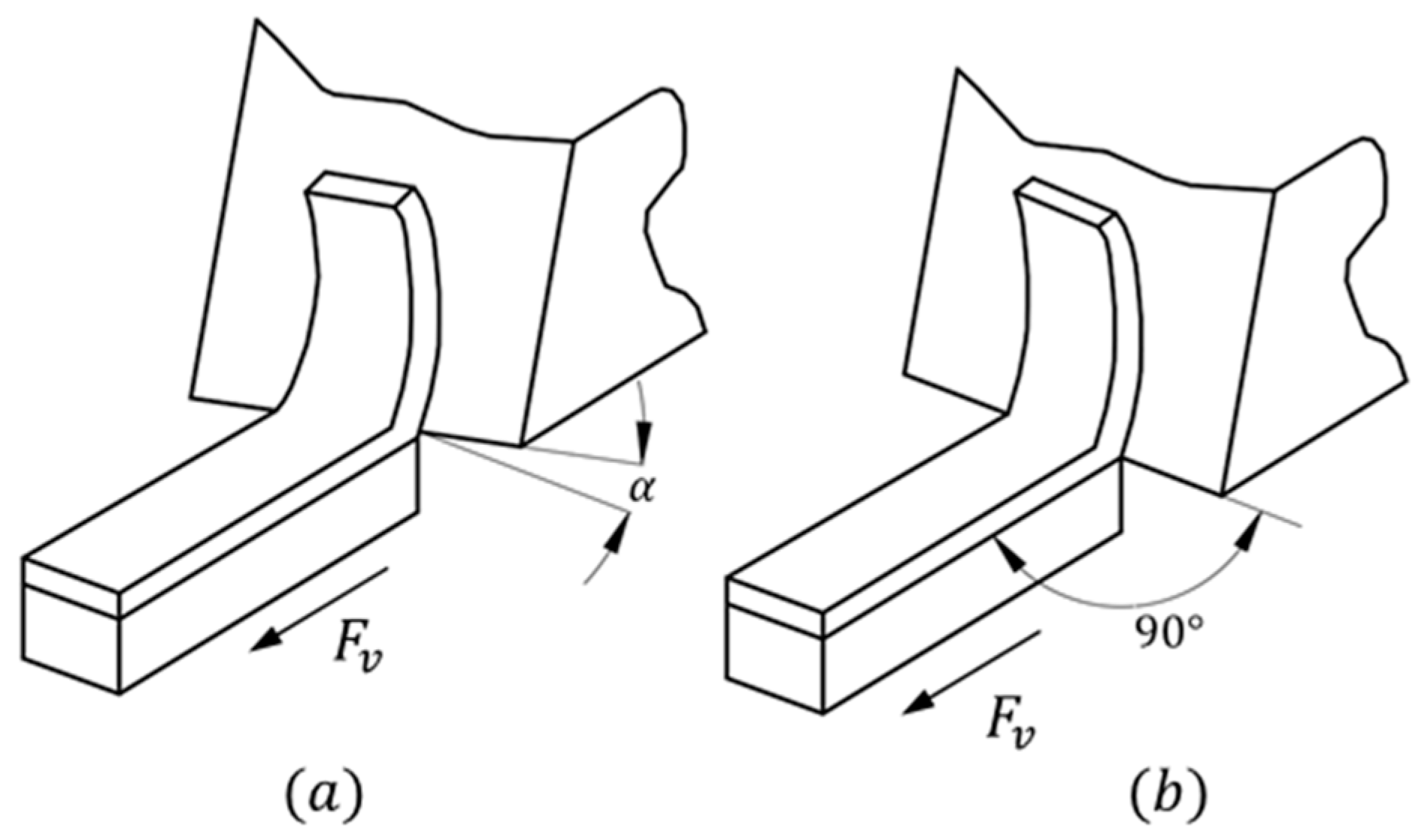
The dynamics of chip removal from the component to be machined are based on the use of a cutting tool, with cutting edges defined by inclination angles. These tools can be used to make straight cuts (perpendicular to the work surface) and oblique cuts (with a tool inclination angle). Figure 1 illustrates these processes.
Most machined components not only involve a specific configuration during the machining operation but are also subjected to different combinations of these operations: turning, rounding, facing, grooving, and threading, among others. There will most likely be different cutting tools, each with its own lead angles, nose roundings, and material characteristics. All these variations in the workpieces will generate different configurations that involve movements and dynamic loads during the machining process. A detailed study of these configurations is required to fully understand these implications. The objective of this article is to show a method for selecting parameters in cutting speed and dept; variations in the angles of attack of the cutting tool that modify the presence of the applied force are not considered in this analysis. For simplicity, it will be assumed that the cut of interest is oblique and directed along the perpendicular axes shown in 
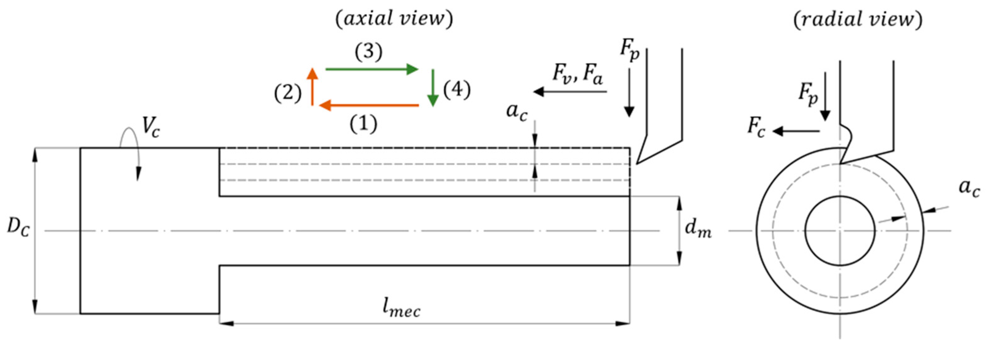
Figure 2, where the expressions for calculating the loads due to contact with the cutting tool and the material are provided by Equation (1), described later.
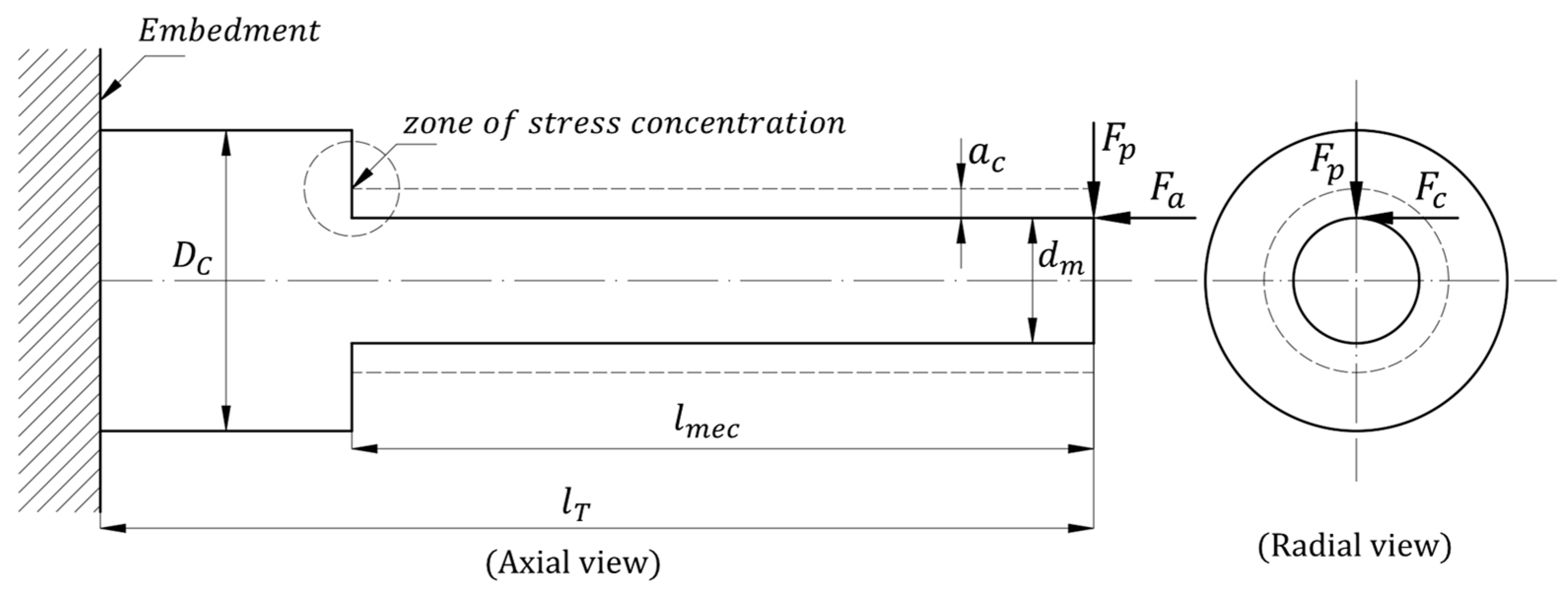
Cutting is carried out by applying a cutting force F c at a tool feed rate F v . The machining process to be considered will be external turning, going from a larger diameter D c to a smaller final finish diameter d m , by applying depth cuts a c over a total machining length l m e c and successively applying cutting passes N p , which are positive integers. The machining process also involves the tangential cutting speed V c and the process quality conditions, defined as the desired surface roughness of the part R c .
The arrows numbered (1) to (4) indicate the direction the cutting tool will take during the machining process. Directions (1) and (2) indicate cutting processes, (3) is rapid retraction, and (4) is positioning for a new cut of thickness a c . The above cycle will be repeated until the requested measurement d m is reached.
The workpiece to be machined has mechanical properties that, depending on the external loads applied to it during the machining process due to contact with the cutting tool and the desired geometric configuration, may tend to fail during the machining process. The most common failure in the machining process, if proper process design (cutting depth, speed, and feed rate, among others) is not considered, will manifest as the fracture of the workpiece during the machining process.
Another, even more dangerous failure (from the author’s perspective), compromises the structural integrity of the component during the machining process, generating cumulative damage that manifests over time and with the use of the component, which can lead to earlier failure than planned in the component design process, decreasing the reliability of the component and generating losses of variable magnitude.
As can be inferred, it is vitally important, when planning the machining process, to consider the loads applied to the material, since these will result in the prevalence of defects or elements that compromise the long-term quality of the component to be machined.
Due to the importance of the chip removal machining process and the consequences of not properly calculating its parameters, many authors throughout history have tried to find methods, through estimation and analysis or combined methods, to choose the best machining parameters that maximize some benefit criterion. Some examples are the work carried out by the authors in [1,2,3], where, based on specific product cases and through direct and indirect measurements, they seek to obtain the best cutting speeds for the process to maximize some other parameter of interest to the process, such as machining cost.
Other authors use computational systems and evolutionary algorithms in combination with maximization requirements for machining processes to estimate the optimal machining parameters, as in [4], where swarm algorithms are used to achieve this goal.
Other authors, such as [5,6], seek precision in the machining process by monitoring and estimating machine tool conditions. Others, such as [7], determine the behavior of the machine process through measurement and comparison with accessories such as lubricants in the process or by monitoring cutting tool characteristics and process-related wear, as in [8,9,10]. Authors such as [11] also seek to define the effect of temperature on the degradation and wear of the process.
Measurement of machining parameters, such as cutting force, is critical for the correct validation of processes. The authors of [12] use measurement mechanisms to determine the magnitude of the force applied to a machining process, thereby estimating the optimal state of the product.
Other authors study the importance of dynamic analysis to eliminate negative effects in machining processes, such as vibration, through modifications in machining conditions, as is the case in [13].
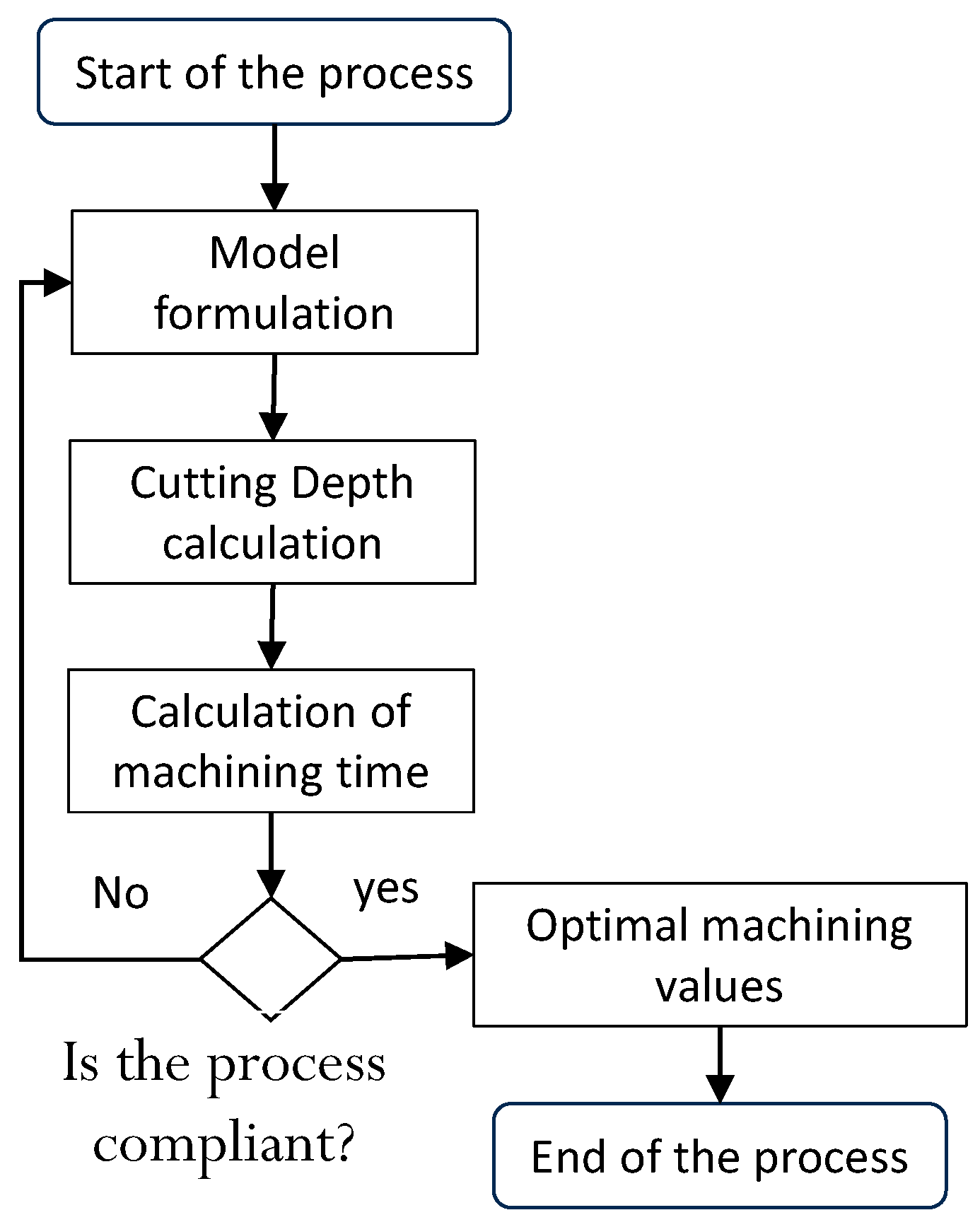
This paper aims to contribute to process optimization and reliability methods by proposing parameter estimation based on the geometry of the component to be machined, its mechanical properties, the power delivered by the machine, and the structural integrity derived from the combination of these parameters, formulating a problem within the field of multi-objective optimization. A bibliographic review of multi-objective optimization applied to machining processes was conducted, and the most relevant results for this research are presented.
Regarding the modeling of multi-objective systems, within the field of research of this article, several works of interest were observed, such as [14] where multi-objective functions are presented, defining the multiple objectives as material removal rate and the rolling factor.
In the article reviewed in [15], the topic of multi-objective optimization is also addressed by defining the parameters of cutting depth, feed, and speed and defining the multi-objective function, such as tool life and operating time.
In the article reviewed in [16] multi-objective optimization is worked on by defining a function defined as a desirability function, where the corresponding optimal values of the input parameters are cross feed, cutting speed, and cutting depth.
In the article shown in [17], a multi-objective optimization mathematical model is presented that considers the spindle speed, cutting tool feed, cutting depth, and process paths as parameters, while the objective function is defined as energy consumption, surface roughness, and machining time.
In the article shown in [18] a multi-goal optimization model is developed where the cutting speed and feed rate are defined as parameters of the objective functions, which are defined as carbon emissions and machining time.
In the article presented in [19] the multi-objective function is designed based on Taguchi experimentation, where the objective functions are cutting quality, production speed, and energy consumption reduction.
In the article presented in [20], a series of advanced multi-objective algorithms for the optimization of turning parameters such as cutting speed, feed, and depth of cut are tested by experimental tests of cutting forces and temperatures, determining material removal rates and surface roughness, and applying four optimization algorithms; values were obtained for the defined functions. This article will be used later to make the comparison with the method of interest. Table 1 shows the results obtained by various tests carried out and taken into consideration by the author.
In the article shown in [21] a multi-objective optimization study of the turning process is carried out based on the Taguchi experiment and by modifying the values of five parameters: tool tip radius, tool holder length, spindle speed, feed rate, and cutting depth, from which the objective functions were constructed: surface roughness, roundness deviation, and material removal capacity.
The article defined in [22] uses neural network-based prediction models to minimize the effect of vibration on the milling process. This article was of interest because the topic it addresses is complementary to that developed in the present article.
The article presented in [23] proposed a multi-objective optimization model for the parameters involved in CNC turning, considering energy consumption in transient and steady states, as well as tool life.
After reviewing the bibliography described in [14,15,16,17,18,19,20,21,22,23], it is concluded that the authors do not present a combination of parameters that involve the machine power, surface roughness, and structural integrity as restrictions to building a mathematical optimization model that involves minimizing the machining cycle time.
Based on the argument previously stated, it is concluded that the topic that the authors develop in this paper is innovative, since it will contribute to the optimization and systematization of the machining process, because it is about presenting an integrative method that takes into account not only the requirements for machining the piece but also restrictions of the machine tool and the work material in order to guarantee the structural integrity and reliability of the machining.

2. Methodology

The methodological proposal for optimizing machining time by chip removal based on ordering algorithms that is developed in this work is shown in the flow diagram in Figure 3.
The end of the process is achieved when, through the formulations, the best combinations of parameters have been obtained that achieve the minimum time and satisfy the process design restrictions.
To achieve this objective, it is necessary to define an appropriate machining strategy that takes into consideration all these factors. This is summarized in the following steps:
  • Define an appropriate machining time calculation model that considers the passes the component will be subjected to.
  • Define a depth of cut calculation model that considers the structural integrity of the component. This involves analyzing the forces and loads on the component according to the requested geometry. To this end, the machining process is defined in the analysis of the turning process.
  • Define the optimization model, considering structural integrity and the criteria involved in the model.
  • Build an algorithm that iteratively executes the steps necessary to determine the depth of cut and cutting speed that satisfy the time minimization and structural integrity criteria.
  • Perform simulations to verify the logical operation of the proposed algorithm.

2.1. Analysis of Cutting Force for Chip Formation

There are different models to characterize the force required to form the chip, depending on the cutting depth. Seeking simplicity in the description of the loads, in the present article the analysis is developed from the oblique cutting model, according to the Kronemberg’s theory, in which only the three force components will be taken into consideration [24,25], thereby restricting the angles that the cutting tool will take and fixing its attack direction. In the study of chip formation, it will be assumed that the tool is a geometric entity formed by the cutting of three planes with a common vertex, where the angle formed by both planes is the smallest possible that meets certain mechanical requirements of friction and energy consumption. The cutting force F c , will be expressed as a function of the remaining force components applied to the workpiece in their respective axes of interest, defined in Equation (1) [24,25]:
F a = F c 5 F p = F c 3 F c = π D c k s F v a c 1000 V c
The resulting force, to which the work material is subjected, from contact with the cutting tool is defined in Equation (2) [24,25] as:
F r e s = F a 2 + F p 2 + F c 2
Figure 4 illustrates the force elements of interest in the chip formation process.

2.2. Restriction Based on the Power Delivered by the Machine’s Engine

The first limitation in the calculation process of the machining process will be the power consumption during machining, which has an upper limit defined by the machine tool’s electric motor, its constituent characteristics, together with the mechanical transmission and other technical configurations; it is not possible to carry out machining processes that require more power than the machine tool can deliver. In a conventional manner, these consumptions are expressed using Equation (3) [14,15]:
P ε = π D c a c F v k s 60,000 ρ T
The equation is based on the process of converting the electrical power required by the machine tool motor. By rearranging all the parameters of the equation to present them with respect to the constant and variable terms, we have Equation (4):
P ε = K 1 a c
For the constant K 1 defined by Equation (5):
K 1 = π D c F v k s 60,000 ρ T
In this way, the electrical power consumption of the machine tool motor is proportional to the tool’s cutting depth. It should be noted that this electrical power corresponds only to that consumed in the machining process; hence, the importance of the efficiency factor ρ T , knowing that the total power of the process will consume a remainder due to the system’s own inertia and losses. The energy delimitation for the process ultimately takes the form of the inequality given in 6:
K 1 a c P ε

2.3. Restriction Based on Surface Roughness

It has been mentioned that one of the benefits of the chip removal machining process is the ability to obtain components with a controlled surface roughness, expressed by the component designer and expressed by Equation (7) [24,25]:
R a 0.008 R c π D c F v 1000 V c 2
where the cutting tool tip rounding parameter R c is involved, Figure 5 illustrates this parameter.
To obtain a roughness lower than that requested by the machining process, it is desirable that it comply with the inequality given in Equation (8).
0.008 R c π D c F v 1000 V c 2 R a
Rewriting the expression obtained as a function of the rounding of the tool tip, we have the inequality defined in Equation (9):
0.008 R a π D c F v 1000 V c 2 R c
For the case study, it will be enough to take the limit value as a function of the cutting speed V c , defining Equation (10):
R c = 1 V c 2 0.008 R a π D c F v 1000 2
Defining the rounding at the tip of the cutting tool as a function of the cutting speed, we have Equation (11):
R c = K 2 V c 2
where the constant K 2 takes the form of Equation (12):
K 2 = 0.008 R a π D c F v 1000 2

2.4. Restriction Based on Structural Integrity

The structural integrity of a machined component is calculated based on the loads to which it is subjected. It is known that stresses near the points of application of concentrated loads reach values much higher than the component’s average. A typical example of this type of loading condition is geometric discontinuities, such as those obtained in the study process. Figure 6 illustrates the applied and resisted load diagram of the workpiece of interest.
The load analysis developed on the workpiece takes into consideration the effects of the cutting forces applied to the workpiece and their effects on the stress concentrator of a machined part in a roughing operation by rolling. Other types of mechanical effects due to the application of the load are not taken into consideration, such as the unbalance effect due to geometric singularities or buckling due to load eccentricities, and the nature of the work material, or vibratory phenomena due to the geometric nature of the workpiece and the driving loads. The study analysis is only stationary due to eccentric loads defined by the diagram in Figure 6.
From the diagram, it can be seen that all geometric factors interact, such as the major and minor diameters of the part, the lengths of the mechanical components, and the direction of load application, to formulate the resulting stresses in the concentrator, defined as the starting point of the discontinuity, defined by the minimum radius of curvature, in this case, the tool radius R c .
It has been observed that the concentration results depend only on the ratios of the geometric parameters involved. Figure 7 illustrates the parameters of interest for constructing the concentration curve, from which the maximum stress of interest to the designer is defined.
The stress concentrator is defined by Equation (13) [26]:
K σ = σ m a x σ p r o m
It is observed that the curves that define the value of the stress concentrator are entered by defining the relationship D c / d m and R c / d m .

2.5. Machining Time

Machining time is defined as the cycle time during which the cutting tool performs a roughing operation. The factors involved in calculating machining time are the cutting tool feed rate and the machining length. Equation (14) [14,15] defines the relationship between these parameters and machining time:
t m e c = l m e c F v

3. Modeling

The load and structural restriction modeling process of the studied machining piece is presented, as well as the equations for the development of the process to obtain optimal machining parameters, cutting depth a c , and the machining time model that will be used to integrate the optimization model used in the proposed method.

3.1. Model for Machining Time Evaluation

The machining cycle time is the function that will be taken as the objective to minimize through the selection of cutting depth and cutting speed. This cycle time is composed of a net machining time, given by Equation (14), and a tool idle movement time; idle movement time is difficult to estimate accurately by technicians during the machining process; therefore, in this article, its structure is proposed as an integral part of the machining time with the modification given in Equation (15):
t = 3 L T 2 F v
The total path to be machined L T is defined by Equation (16) as:
L T = N p l m e c
N P represents the number of machining cycles or number of passes that the cutting tool has to make to obtain the final diameter d m . This number of iterations must be an integer; therefore, it is calculated from the rounding up function ( R s u p ) dependent on the measurements of the material to be machined ( D c ) and the desired machining ( d m ), as well as the cutting depth ( a c ) using Equation (17):
N p = R s u p D c d m 2 a c
The total machining time, then, takes the form given by Equation (18):
t = 3 l m e c 2 F v R s u p D c d m 2 a c
For work design purposes, the depth of cut will be constant and must be consistent with the number of iterations in the machining cycle; that is, once the depth of cut has been calculated, it must be consistent with the iterations and therefore must be adjusted to it. This will involve an adjustment calculation defined by Equation (19):
a c σ = D c d m 2 N p
where a c σ represents the final cutting thickness, once the best expression for cutting depth is found, such that a c σ a c .
For the design of the machining process, this will involve entering a suboptimal machining time region, which at most will be close to the optimum, but, in most cases, will not be optimal.

3.2. Model for Determining Cutting Depth Based on Structural Integrity

It is illustrated in the diagram of the study component in Figure 8, where emphasis is placed on the application of loads due to the shear force, assuming that the embedment is adequate at the contact point and there is no risk of failure due to tie-in, therefore, the failure factor due to embedment will not be taken into consideration.
The diagram shows the effect of the applied loads due to the shear action in combination with the desired geometry, generating a stress concentrator due to the combination of both parameters (load-geometry), which is the primary element of study as a structural element.
The effect of the maximum stress located at a distance l m e c and in a diameter d m + 2 a c can be noted, just before the final machining this effect will occur, at the time of the final machining pass. It is assumed that the cutting thickness a c is constant throughout the process, and it must be determined based on the stress concentrator due to the machining process.
The stress behavior in the stress concentrator is not only characterized by the effect of the load but also by the geometric relationships between the final finished diameter d m and the work material diameter D c , as well as the geometry of the relief generated during the machining process and defined by R c .
As shown in Figure 7, the smaller the ratio of relief to finished diameter ( R c / d m ), the greater the effect of the stress concentrator. The same is true for the ratio of work material diameter to final finished diameter ( D c / d m ). The higher the ratio, the greater the effect of stress concentration.
It is observed that the parameter D c / d m is fixed, defined by the geometry of the machining process, while the parameter R c / d m depends on the cutting tool radius R c , which will control the effect of the stress concentrator. Figure 7 shows that this relationship can avoid asymptotic values by fulfilling the type of restriction given in inequality Equation (20):
R c d m 0.05
For the case study, it will be enough to state this inequality in the form of Equation (21):
R c = 0.05 d m
This ensures that the stress concentration does not exceed values four times the average stress applied to the workpiece. In this research proposal, the tool tip radius will characterize the stress concentrator of the component under study.
Figure 9 illustrates the load and moment diagram with respect to the point located on the axial axis of maximum effect (point 0). It should be noted that the workpiece origin is defined at the external machining starting point (point A), and the machine origin is defined at the endpoint of the chuck or workpiece clamp (point 0). Under this load modeling process, the effects of bending, shear, and torsion are taken into consideration, phenomena due to the load applied by the cutting tool.
The resulting bending moment M r e s and the resulting applied force F r e s are defined and related by means of axis translation and vector simplifications given in Equation (22):
M r e s = R x F r e s + M A F r e s = F a i ^ F p j ^ + F c k ^ R = l T i ^ + d m 2 j ^
The moment M A is defined by Equation (23):
M A = d m 2 j ^ x F r e s
In vector form, we have the structure M A defined by Equation (24):
M A = i ^ j ^ k ^ 0 d m 2 0 F a F p F c = d m 2 F c i ^ + d m 2 F a k ^
For the moment R x F r e s the Equation (25) is defined as:
R x F r e s = i ^ j ^ k ^ l T d m 2 0 F a F p F c = d m 2 F c i ^ + l T F p j ^ + d m 2 F a l T F p k ^
This implies a resulting moment defined by Equation (26):
M r e s = d m F c i ^ + l T F p j ^ + d m F a l T F p k ^
The load analysis presented does not take into consideration the dynamic-vibratory effects of the workpiece; it assumes a balanced stationary load, leaving aside vibrations due to imbalance and the resulting phenomena that the turning process would imply.
From the vector formulation, one can calculate the average stresses applied to the workpiece, which take the form given by Equation (27):
σ P r o m = σ A x i a l + σ F l e x i n g
Substituting Equations (22)–(26) into Equation (27) gives the form of the average stress given by Equation (28):
σ p r o m = F r e s π d m 2 + a c 2 + M r e s d m 2 + a c 1 4 π d m 2 + a c 4
where M r e s takes the form given by Equation (29):
M r e s = d m F c 2 + l T F p 2 + d m F a l T F p 2
Substituting Equation (1) into the magnitude of the resulting force F r e s gives the expression given by Equation (30):
F r e s = π D c a c k s F v 5000 V c 2 + π D c a c k s F v 3000 V c 2 + π D c a c k s F v 1000 V c 2
Simplifying Equation (30) gives the form given by Equation (31):
F r e s = π D c a c k s F v V c 1 5000 2 + 1 3000 2 + 1 1000 2
The reduced form of the magnitude of the resultant force takes the form of Equation (32):
F r e s π D c a c k s F v V c K F
For the constant K F defined by Equation (33):
K F 0.001073
The magnitude of the bending moment M r e s , expressed in terms of its force components given by Equation (1), has the form given by Equation (34):
M r e s = π D c a c k s F v V c d m 1000 2 + l T 3000 2 + d m 5000 l T 3000 2
In a simplified way, we have the expression for the bending moment M r e s given by Equation (35):
M r e s = π D c a c k s F v V c K M
For the term K M defined by Equation (36):
K M = d m 1000 2 + l T 3000 2 + d m 5000 l T 3000 2
Substituting Equations (32) and (35) into the average stress given in Equation (28) gives Equation (37):
σ p r o m = 4 F r e s π d m + 2 a c 2 + 32 M r e s d m + 2 a c π d m + 2 a c 4
Simplifying, we have the expression given in Equation (38):
σ p r o m = D c a c k s F v V c d m + 2 a c 2 4 K F + 32 K M d m + 2 a c
The stress manifested in the component to be machined will depend on the parameters: d m , D c , R c ; arrangements defined by the design of the machining process, which leads to geometric inequality in the axial section, such that the stress concentrator described above appears; therefore, the maximum stress, applied in the stress concentrator and of interest to maintain the structural integrity, is defined by Equation (39) as:
σ m a x = S a c = K σ σ p r o m
Substituting Equation (38) in (39) gives the form given by Equation (40):
σ m a x = K σ D c a c k s F v V c d m + 2 a c 2 4 K F + 32 K M d m + 2 a c
The structural integrity of the piece to be machined will be maintained as long as the maximum stresses ( σ m a x ) present in the piece, due to the machining process, are less than the elastic resistance module ( S y ), and related, in a simple way, by a safety indicator ( N 1 ) in the way shown in Equation (41):
N = S y σ m a x 1
The critical value of elastic failure will occur when N = 1 , such that the structural integrity expression is given by Equation (42):
σ m a x = S a c = S y
Substituting Equation (40) into Equation (42) gives the structure given by Equation (43):
K σ D c a c k s F v V c d m + 2 a c 2 4 K F + 32 K M d m + 2 a c = S y
Thus, for there to be no failure in the material due to the machining process, the inequality shown in Equation (44) must be met:
S a c = K σ D c a c k s F v V c d m + 2 a c 2 4 K F + 32 K M d m + 2 a c S y
Which will be the form finally adopted by the structural restriction for the piece to be machined, depending on the machining parameters and the cutting depth of the working tool.

4. Analysis of Results

Based on the theory presented, the machining time optimization model t is presented, which will involve the cutting depth a c as its defining parameter, as well as the process restrictions defined in Section 3, thereby establishing the iterative algorithm to search for parameters and a test consistent with the limitations established for the study model to finally obtain the optimal cutting depth parameters a c and cutting speed V c .

4.1. Optimization Model Approach

The machining process optimization model proposed to minimize machining time takes the form proposed by Equation (45):
M i n t = 3 l m e c 2 F v R s u p D c d m 2 a c
The restrictions requested for the calculation of this process are of the structural, energy, and surface finish type, defined by the relationships given in Equation (46):
K 1 a c P ε K σ D c a c k s F v V c d m + 2 a c 2 4 K F + 32 K M d m + 2 a c S y R c = m a x 0.05 d m ,   K 2 V c 2
For the coefficients defined from Equation (47):
K 1 = π D c F v k s 60,000 ρ T K 2 = 0.008 R a π D c F v 1000 2 K F 0.001073 K M = d m 1000 2 + l T 3000 2 + d m 5000 l T 3000 2 K σ = K σ R c , D c , d m M a x 0.05 d m ,   K 2 V c 2   D c d m
In this proposed model, the cutting depth a c will depend on the process parameters: material strength, the machining process to be performed, and the power available to carry out the process, delivered by the machine tool motor.
Table 2 shows the dynamic parameters used to define the process provided by cutting tool manufacturers for work on conventional machine tools, in this case, a parallel lathe. All parameters are constant and fixed except for the cutting speed, which takes values defined by intervals according to the roughing or finishing operation.
Table 3 shows the typical surface roughness values, requested during the chip removal machining process depending on the application of the component to be machined.
Based on the available technical parameters and the requested geometric data, it is possible to begin the process of selecting the optimal speed, which will be linked to the cutting depth, and will comply with the proposed machining time indicator, subject to the imposed restrictions.

4.2. Machining Parameter Optimization Algorithm

The general algorithm proposed for the search process to determine the optimal speed from which the best cutting depth will be obtained, complying with the structural integrity restrictions for the machining process under study, is shown in Figure 10.
The process of analyzing values for machining begins by estimating the initial maximum cutting depth of the process a c ε from the geometric parameters K 1 , the electrical power available from the electric motor P ε and the range of minimum cutting speeds V c , m i n and maximum cutting speed V c , m a x to generate the search and selection of better parameters. In this global process, it is observed that the average stationary energy of the machining process E p r o m is generally estimated as a reference that the process consumes energy within the parameters limited by the power of the machine tool motor P ε . This energy is only an average; if a greater depth in the subject is required, a dynamic study of consumption would have to be completed, a subject outside the objectives sought by this paper.
The algorithm shown in Figure 11 illustrates the procedure for estimating the adjusted cutting depth a c σ applied to the machining process. It can be observed how, by seeking to comply with the structural integrity restriction function, a cutting depth is obtained in accordance with the same a c ε , which will be adjusted according to the rounding of the number of passes to finally obtain the adjusted cutting depth a c σ consistent with the machining process and with a decrease in the cutting depth defined by a c .
The optimization process and search for the shortest machining time are developed using the descending algorithm shown in Figure 12, where the shortest average machining cycle time t is finally estimated according to the cutting depth that best preserves the structural integrity of the machined part.

4.3. Application Example

To illustrate the operation of the proposed algorithm, the machining of a component with the geometric characteristics shown in Figure 13 is defined.
The manufacturing conditions of the test piece are shown in Table 4.
These parameters were input into the processed algorithm (see Appendix A), producing the following graphs for a speed range defined by the cutting tool manufacturer and given the machine tool’s constraints:
For the cutting tool nose radius, recommended to meet the surface roughness restriction, Figure 14 illustrates its variation with respect to cutting speed.
Figure 15 shows the comparison of machining time with respect to cutting depth and stress derived from the machining process S a c when the cutting speed varies within the range recommended by the cutting tool manufacturer.
Figure 16 shows the depth of cut applied compared to the number of passes required to reach the requested machining size and the time consumed in this process.
Figure 17 shows the comparison between the machining time, the average electrical power consumed by the electric motor, and the average energy consumed by the process.
To measure the behavior of the proposed method, a comparison is made with the test piece defined in [20] and the parameters obtained between both methods are compared. Table 5 shows the properties reported by the author together with the properties necessary to carry out the simulation with the developed model, such as specific cutting pressure k s and electric motor power P ε .
The geometry of the piece machined by the author in [20] is characterized only by the outer diameter because single-pass cuts are made in his experiment. For the model proposed in this article, it is necessary to define a diameter d m to characterize the maximum load due to the stress concentrator; a smaller diameter d m = 58   m m will be proposed arbitrarily in order to perform the calculation and analysis of the maximum load applied to the workpiece, thereby trying to replicate, with the model itself, the design of its working conditions.
From the development of the problem posed and taking into consideration the cutting speed V c reported by the author, the values shown in Table 6 were obtained.

5. Discussion

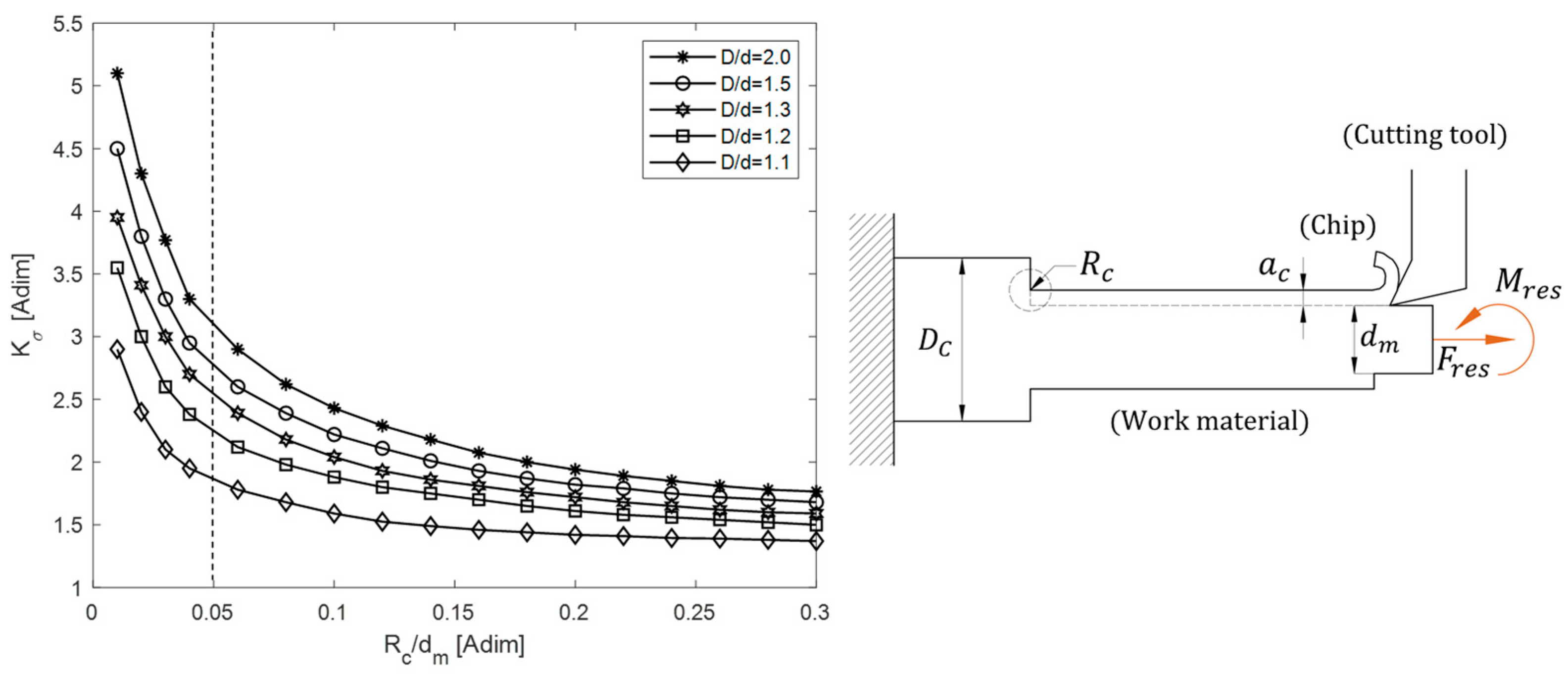
The developed model allows, based on the results obtained in the simulation, exploration of the behavior of the cutting speed V c within the ranges recommended by tool manufacturers and its relationship with machining parameters in the study piece, such as the optimal cutting depth a c σ that will guarantee the reliability and structural integrity of the process. The variation of the cutting tool nose radius R c and its variation with the cutting speed V c can be observed. It is observed that at higher cutting speeds, the cutting tool nose radius is smaller, which meets the requested roughness requirements. 
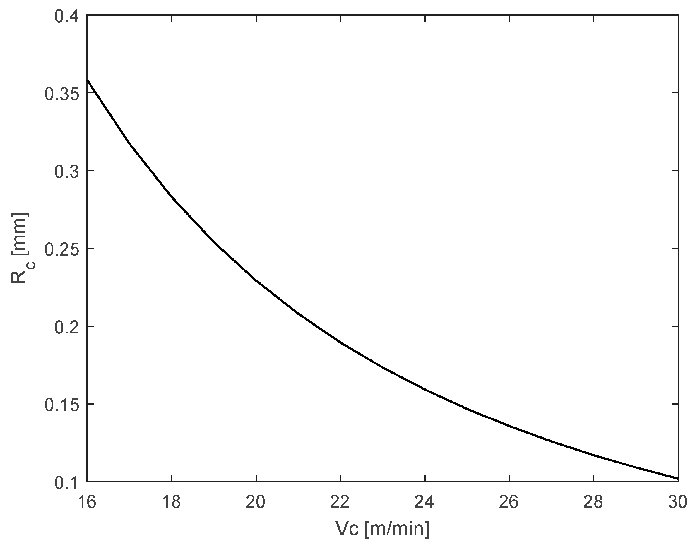
Figure 14 illustrates this process.
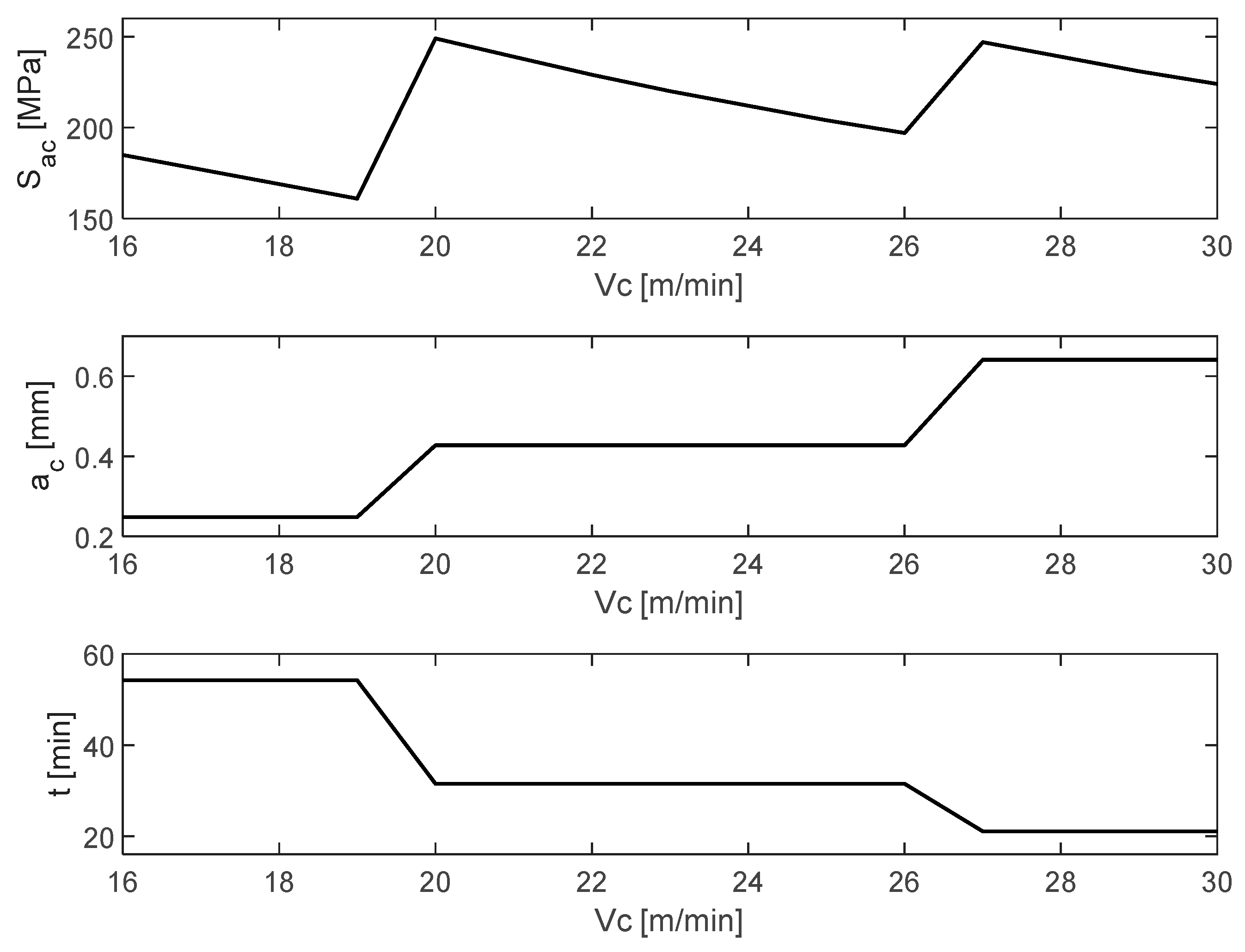
Among the important findings are values that, although permissible by the machining process, should not be selected since they generate the risk of compromising the structural integrity due to the stresses that will be obtained in the cutting process of the material S a c . Figure 15 illustrates the behavior of these cutting parameters, crests and valleys, with respect to the stress S a c generated by the optimal cutting depth a c σ and the time t consumed in the machining process. From this data, the professional will have more information on which values to take according to their technical requirements.
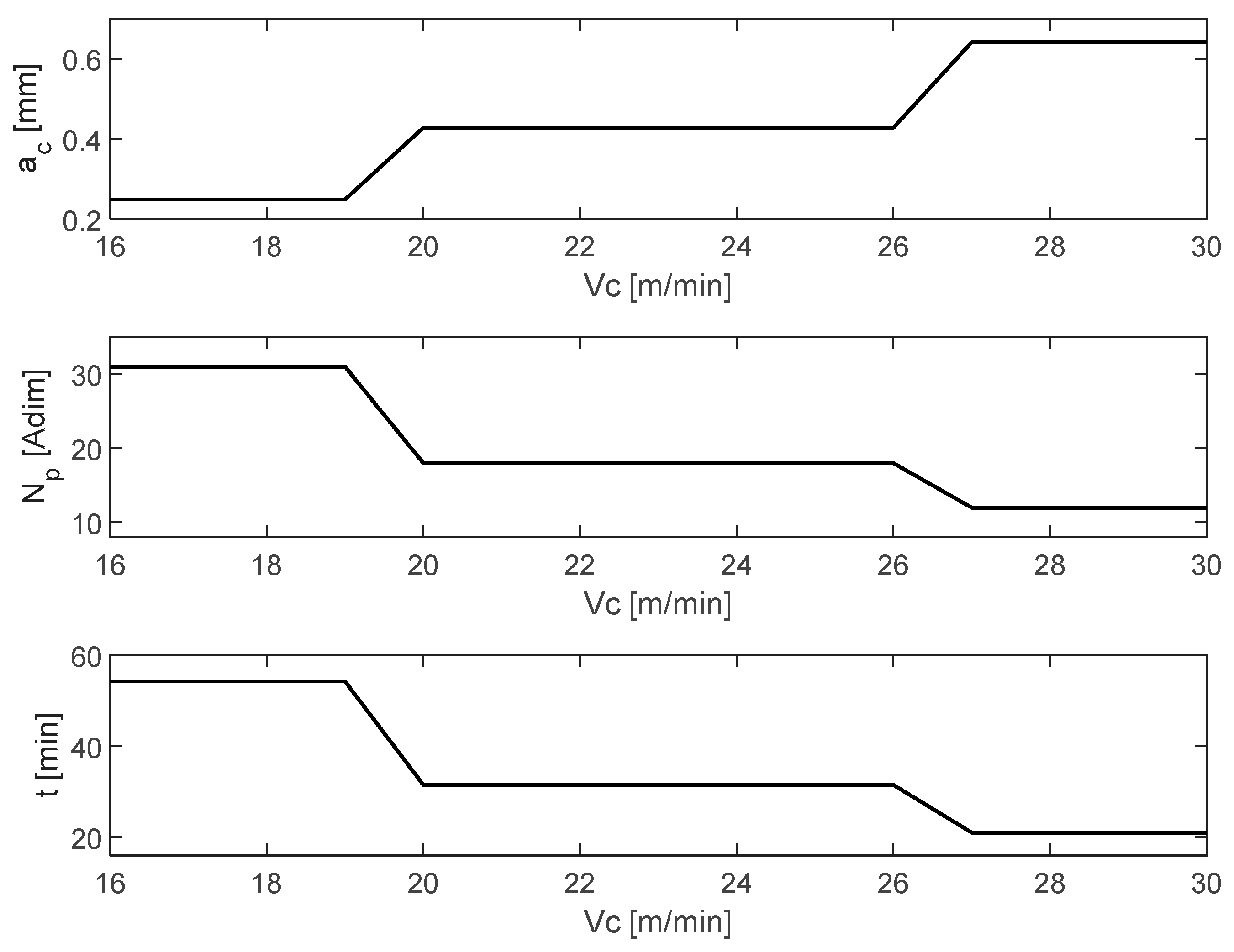
According to the allowable cutting speed V c , there will be optimal cutting depth values a c σ in intervals of values in cutting speed V c , which will generate the same effect in terms of number of machining cycles N p and machining time t . Figure 16 illustrates this process in such a way that in practice, if only these parameters are involved, it does not matter whether you work at one cutting speed or another that is in the same interval where the machining time t is due to the number of machining cycles N p being equal.
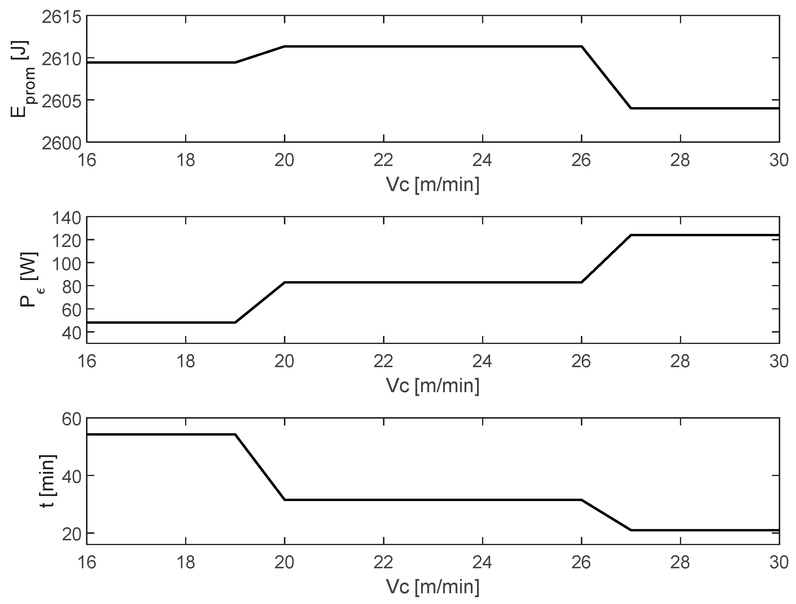
According to the restrictions imposed on the model, the algorithm will always seek to meet viable conditions within the range of allowable cutting speed V c and adjusting cutting depth a c σ for the machining process in such a way that the average energy consumed E p r o m will try to balance between elapsed time t and consumed power P ε , showing a quasi-constant behavior as observed in Figure 17.
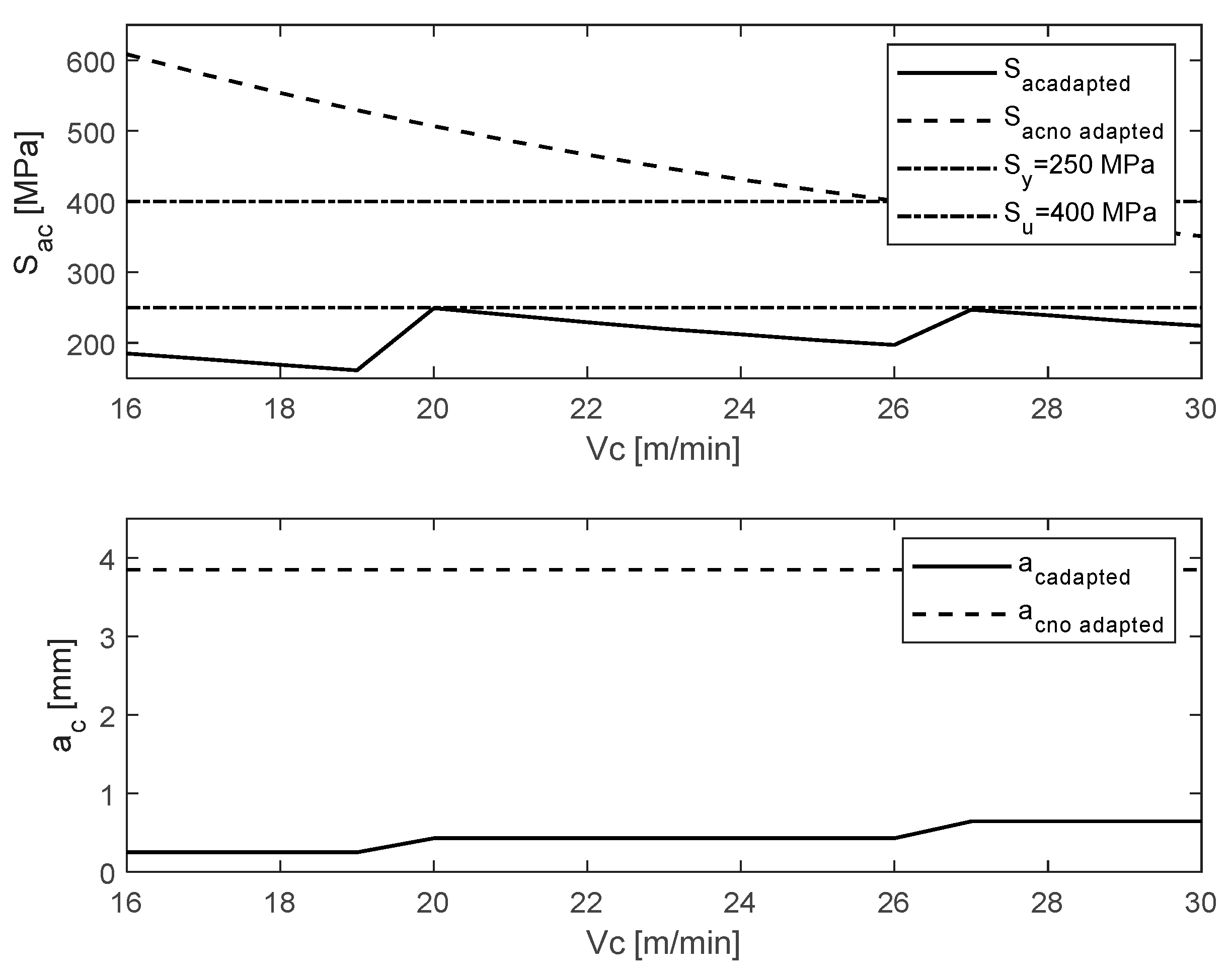
Table 7 summarizes the values obtained by varying the cutting speed within the permissible parameters for the process. Among the values presented in Table 7, it is important to highlight the column corresponding to the calculation of the maximum stress S a c ε , calculated by using the maximum possible cutting depth a c ε due to the cutting power provided by the machine tool motor P ε . With the calculation of this maximum stress it is possible to justify why, despite the fact that the machine tool allows through the power delivered by it P ε , it is not advisable to use the maximum cutting thickness a c ε , because this will give rise to a stress S a c ε that in most of the cutting speed values used exceeds the ultimate allowable stress S u by the test material. Moreover, from that maximum thickness a c ε under the test with all the test cutting speeds V c , the estimated maximum stress S a c ε exceeds the yield strength S y of the test material, which will lead to exceeding the elastic limit of the workpiece, generating, at least, plastic deformations and thereby compromising the machining process.
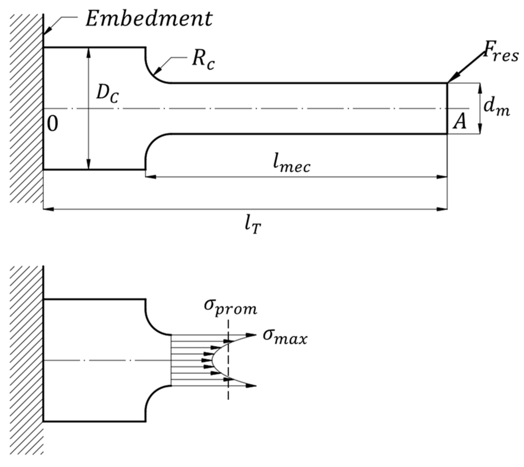
Figure 18 illustrates the behavior of the stress obtained with respect to the optimal cutting depth S a c and the initial cutting depth S a c ε defined by the characteristics of the electrical power delivered by the machine tool.
The analysis presented in this article is focused on manual machining; however, the presented model can, in theory, provide cutting depth a c values for automatic machines operating at higher cutting speed V C 
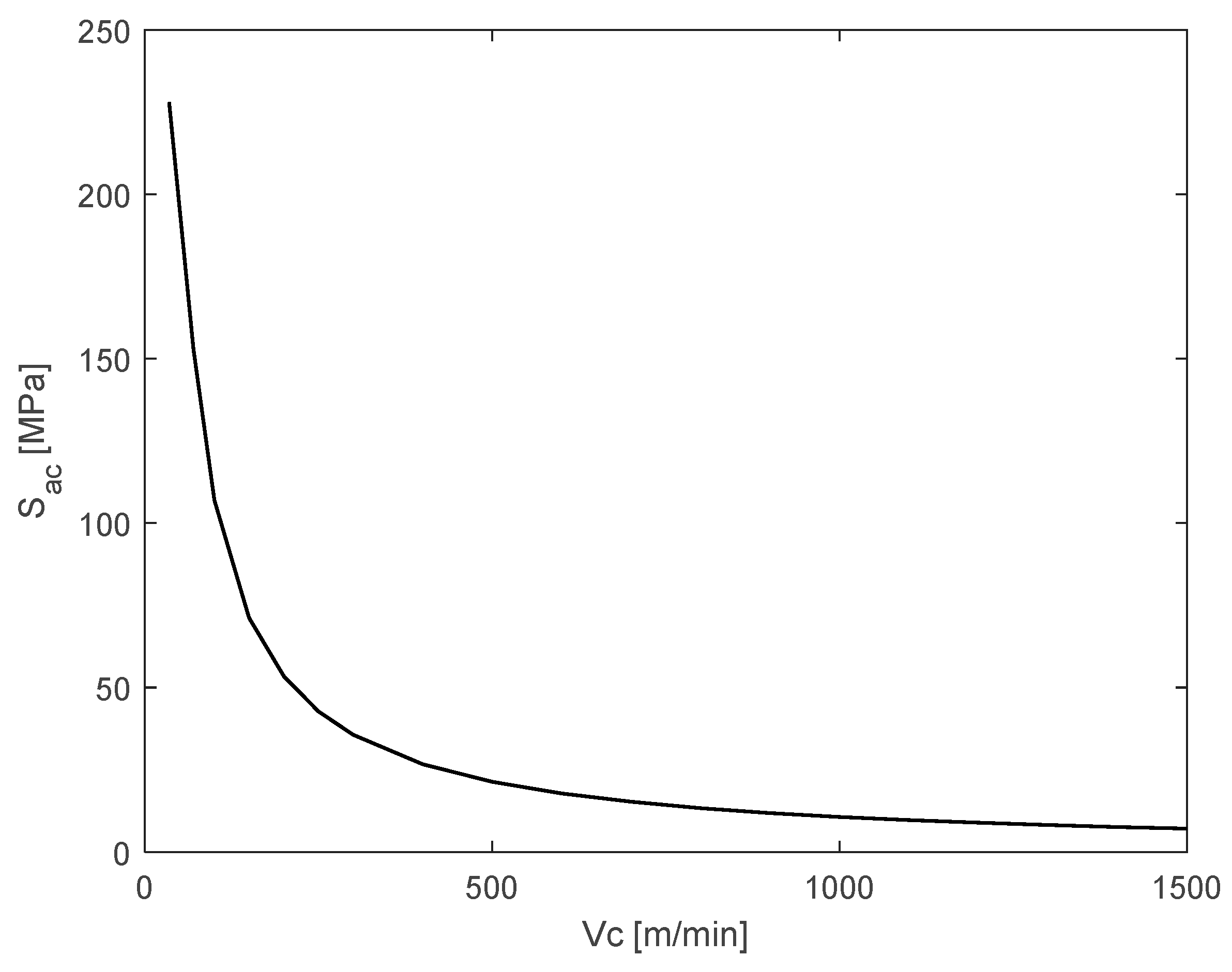
, from which an analysis of the variation of high cutting speeds for automatic machines is presented, it was observed that, at higher cutting speeds involved in the machining process, the resulting effort of the process is lower, and therefore, the reliability in the process increases significantly, which results in a point to consider when discussing the replacement of equipment or the simulation of the process under other allowed parameters of cutting speed for other types of machinery. Figure 19 summarizes the theoretical values when varying the speed from 35 to 1500 m / m i n and the effort obtained from the process S a c .
Other parameters, such as cutting depth, are not considered because starting at values of 70 m/min, the minimum required cutting depth is a c = 2.56   m m , the power consumed by the electric motor remains at P ε = 497   W , the number of passes is N p = 3 , and the machining time is t = 5.25   m i n .
It should be noted that these simulated high speeds do not consider imbalances, vibration imperfections, or other loading factors, which must be analyzed in greater detail for high-speed analysis. Future work involves strengthening the decision-making model by incorporating more factors from the machining process. For now, the work completed is considered satisfactory.
The method shown is scalable to other types of materials and machines under the same load configuration and geometric configurations; it will be enough to define the parameters of the materials in the proposed model, taking as references the tables recommended by manufacturers of cutting speeds, feeds, and properties of the working materials, exemplified in Table 2 and Table 3.
To analyze the characteristics of the developed model, a comparison is made with the model proposed in [20]. Based on the results presented therein and using the optimal cutting speed defined by the author, the results shown in Table 6 are obtained.
To draw conclusions from the comparison, some observations must be made:
  • The model analyzed in [20] considers the optimization criterion defined as the material removal rate (MRR).
  • The proposed model uses the final diameter required for the workpiece dm as a necessary measure for calculating structural integrity and process reliability.
  • The optimization criterion in the proposed model is the machining time and the adjustment of the cutting depth relative to the machining cycle, in conjunction with the available cutting speed Vc.
From which it can be observed that, taking the same criteria of cutting speed V c , tool feed F v , geometric parameters defined only in roughing operation, there is a variation in the calculation of the cutting force, approximately half of the available. This discrepancy can be explained as a combination of different factors, such as the angular configuration of the tool used in the process described in [20] and the oblique cutting model proposed in this article, the structural integrity factor, and geometric factors involved in the process. The obtained roughness parameter R a is practically the same in both models. These models and subsequent adjustments will be studied in greater depth in future work.
There are several topics to be addressed further under the load analysis framework described above. One of these is dealing with various load configurations, i.e., parts subjected to turning, facing, parting, etc., since these load configurations will give rise to other stress and resistance configurations later.
Another topic of interest is to strengthen the model through a buckling analysis under eccentric loads to determine the vibratory effect of the component to be used. This loading effect is not considered; however, for various load configurations and geometrical characteristics of the part to be machined, will contribute to poor machining.
Following the line of effects due to configuration on mechanical properties, geometry of the part, and dynamics imposed on the system by cutting speed, the vibratory effect of these factors must be analyzed and verified to determine whether together they do not contribute negatively to the machining process, manifesting as imbalances and generating deficiencies in surface machining and machining tolerances.

6. Conclusions

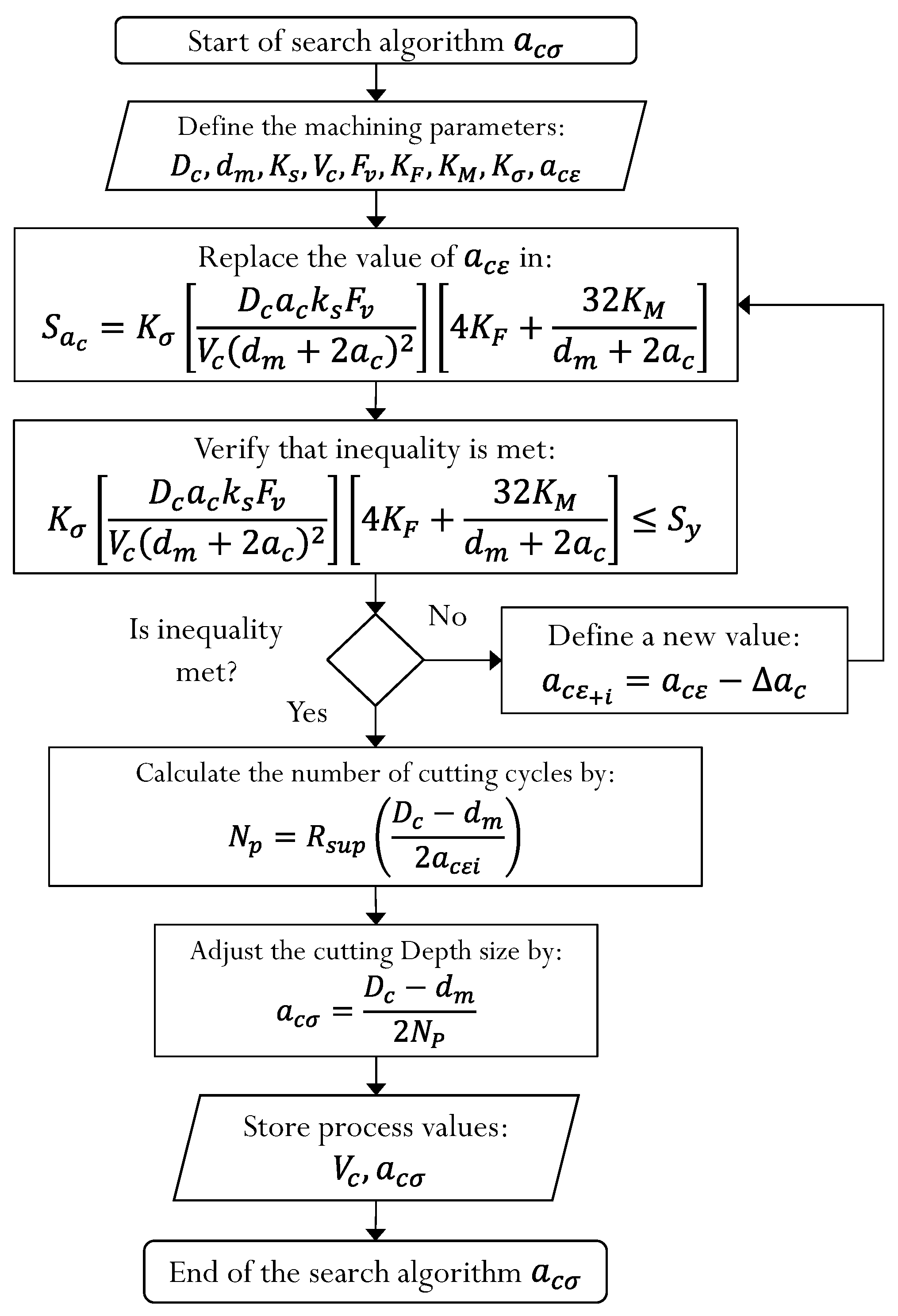
In this paper, a new method is presented for the calculation of the depth of cut a c and cutting speed V c focused on machining by chip removal in turning process under roughing operation. This method takes into consideration the loads applied to the workpiece derived from the interaction between cutting tool and work material, as well as the dynamics requested to the machine tool, characterized in the electric power of the motor P ε and the surface finishing conditions required by the surface roughness R a , integrated in an optimization model that is solved by an iterative search algorithm, which preserves the structural integrity by interpolating parameter values that meet the requested requirements according to the mentioned limitations.
By implementing the parameter search method defined by the iterative algorithm, it is guaranteed that the deflection in the part, as well as the eccentric load due to the cutting, will be within the requested restrictions, thereby ensuring the quality of the surface finish. If a cutting depth a c greater than estimated is applied, there is a risk of deflection in the part, which could lead to vibratory phenomena that would contribute to the deterioration of the surface roughness R a , also affecting the dimensional tolerances requested from the workpiece. Under the considerations of defined load analysis, the proposed method is satisfied since it is consistent with the classical theories of structural failure of mechanical components, successfully integrating the optimal machining parameters of interest.
From this article, an analytical methodology is made available to the machining process analyst estimating the optimal cutting depth a c and cutting speed V c , according to the optimal machining time t , based on structural behavior analysis of the workpiece. With this, it is guaranteed that the workpiece, in an analytical manner, is reliable under the configuration process of the material parameters and the requested geometry. It consumes the minimum electrical power P ε necessary, according to the conditions of the machine tool motor, and that it guarantees to have the minimum surface roughness quality R a required by the designer of the piece.

Author Contributions

Conceptualization, A.M.-G.; methodology, A.M.-G.; software, A.M.-G., N.F.G.-R., and I.R.-C.; validation, A.M.-G., N.F.G.-R., and I.R.-C.; formal analysis, A.M.-G.; investigation, A.M.-G.; resources, A.M.-G.; writing—original draft preparation, A.M.-G. and N.F.G.-R.; writing—review and editing, A.M.-G., N.F.G.-R., and I.R.-C.; supervision, N.F.G.-R. and I.R.-C.; funding acquisition, A.M.-G. All authors have read and agreed to the published version of the manuscript.

Funding

This work was funded by the Ministry of Higher Education, Science and Technology (MESCyT) of the Dominican Republic through the Fondocyt with allocation code 2020-2021-3A9-069.

Data Availability Statement

Data are contained within the article.

Acknowledgments

This work was supported by the National Fund for Innovation and Scientific and Technological Development (Fondocyt) issued by the Ministry of Higher Education, Science and Technology (MESCYT) of the Dominican Republic, in collaboration with the Pontifical Catholic Mother and Teacher University (PUCMM). We are grateful for all the support provided by these organizations for the completion of this research.

Conflicts of Interest

The authors declare no conflicts of interest.

Nomenclature

ParameterDefinitionUnits
i ^ , j ^ , k ^ Unit vectors, for defining the direction of shear forces A d i m
a c Cutting depth m m
a c σ Optimum cutting depth m m
a c Cutting depth adjustment parameter m m
D c Major diameter of the work material m m
d m Machined (minor) diameter of the workpiece m m
E p r o m Average steady-state energy consumed by the process J
F c Tangential shear force N
F a Axial cutting force N
F p Radial cutting force N
F r e s Resulting machining force N
F r e s Vector resulting machining force N
F v Feed rate of the cutting tool m m / m i n
K 1 Constant of electrical power parameters N / s
K 2 Surface roughness parameter constant m 3 / s 2
K F Constant of proportionality to the load force A d i m
K M Constant of proportionality to the load moment m m
k s Cutting pressure, interaction between tool and material M P a
K σ Stress concentration factor A d i m
l m e c Machining length m m
L T Total path to be machined m m
l T Total length of the workpiece m m
M r e s Resulting moment, applied to the work material N m m
M r e s Vector resulting moment, applied to the work material N m m
M A Moment about point A of the force F r e s N m m
M A Vector moment about point A of the force F r e s N m m
N p Number of passes to the cut A d i m
N Structural safety factor for loading conditions A d i m
N i n d Number of iterations for the analysis of the algorithm A d i m
P ε Variable electrical power supplied to the machine tool W
R Application vector of the resulting moment M r e s m m
R a Surface roughness requested for machined part m m
R c Radius of the cutting tool m m
ρ T Energy efficiency factor A d i m
S a c Stress due to cutting material at depth a c M P a
S a c ε Stress due to cutting material at depth a c ε M P a
S u Ultimate strength of the working material M P a
S y Creep resistance of the work material M P a
σ m a x Maximum stress due to the machining process M P a
σ p r o m Average stress due to the machining process M P a
σ A x i a l Axial stress resulting from the machining process M P a
σ F l e x i n g Bending stress resulting from the machining process M P a
t Total machining process time s
t m e c Net machining time s
V c Tangential cutting speed m / m i n
V c , m i n Minimum cutting speed defined by the work material m / m i n
V c , m a x Maximum cutting speed defined by the work material m / m i n

Appendix A

Programming to Obtain Total Process Parameters

% Programa para Calcular la Profundidad de Corte en el proceso de
% mecanizado por arranque de viruta
% Abraham Manilla Garcia
% 22 de mayo de 2025
%--------------------------------------------------------------------------
clear all
clc
% DEFINICION DE CARACTERISTICAS DESEABLES PARA EL DISEÑO DEL PROCESO
Fv=60; % Velocidad de avance de la herramienta de corte [mm/min]
Ks=1700; % Presion especifica de corte del material de trabajo [MPa]
Sy=250; % Resistencia a la fluencia acero dulce [MPa]
Pe=746; % Potencia consumida por la Maquina Herramienta [W]
Rho_T=0.7; % Factor de eficiencia del proceso de mecanizado [Adim]
Ra=0.002; % Rugosidad superficial para superficies mecanizadas en general [mm]
Vc=1500; % Velocidad de corte minima [m/min]
% Vcmax=30; % Velocidad de corte maxima [m/min]
% DVc=1; % Incremento de la velocidad de corte [m/min]
DeltaAc=0.2; % Parametro de disminucion del tamaño de corte [mm]
% DEFINICION DE PARAMETROS GEOMETRICOS DE LA PIEZA DE TRABAJO
Dc=25.4; % Diametro mayor de la pieza de trabajo [mm]
dm=10.0; % Diametro menor, deseado [mm]
lmec=70.0; % Longitud del mecanizado [mm]
lT=110.0; % Longitud total de la pieza a tornear medida desde la punta de mordazas [mm]
% DEFINICION DE CONSTANTES K1, K2
K1=(pi∗Dc∗Fv∗Ks)/(60000∗Rho_T);
K2=(0.008/Ra)∗((pi∗Dc∗Fv)/1000)^2;
Rc2=0.005∗dm; %Redondeo de la nariz de HTA para evitar asintotas
Acsup=Pe/K1; % Cota superior para la profundidad de corte [mm]
Acini=Acsup; % Almacenamiento de profundidad de corte inicial [mm]
KM=sqrt(((dm/1000)^2)+((lT/3000)^2)+(((dm/5000)-(lT/3000))^2));
Kf=0.001073; % Parametro de proporcionalidad de coeficientes
% ANALIZAR COMPORTAMIENTO DE VELOCIDADES
Rc1=K2/(Vc^2); % Analisis de redondeo de la nariz de Hta.
if Rc1 > Rc2
Rc= Rc1;
elseif Rc1 < Rc2
Rc = Rc2;
end
Ksigma=-10*(Rc/dm)+3.5; % Definicion de funcion de concentrador de esfuerzo Ksigma
% ESTIMACION DE PROFUNDIDAD DE CORTE ac
P1=(Dc∗Acsup∗Ks∗Fv)/((Vc)∗(dm+2∗Acsup)^2);
P2=(4∗Kf)+((32∗KM)/(dm+2∗Acsup));
Sac=Ksigma∗P1∗P2;
while Sac > Sy
Acsup=Acsup-DeltaAc;
P1=(Dc∗Acsup∗Ks∗Fv)/((Vc)∗(dm+2∗Acsup)^2);
P2=(4∗Kf)+((32∗KM)/(dm+2∗Acsup));
Sac=Ksigma∗P1∗P2;
end
Np=ceil((Dc-dm)/(2∗Acsup)); % Numero de pasadas por corte (enteras)
Acajus=(Dc-dm)/(2∗Np); % Ajuste de la profundidad de corte al tamaño de la pasada
% CALCULO DE TIEMPO DE MECANIZADO
Tm=((3∗lmec)/(2∗Fv))∗Np;
% CALCULO DE LA POTENCIA CONSUMIDA POR EL MOTOR ELECTRICO
Pec=Acajus∗K1;
% CALCULO DE LA ENERGIA PROMEDIO CONSUMIDA POR EL PROCESO DE MECANIZADO
Eprom=Pec∗Tm;

References

  1. Botak, Z.; Pisačić, K.; Horvat, M.; Tomić, T. Determination of Optimal Machining Parameters Based on Roughness and Vibration Measurements of Pieces Produced by Whirling on a Lathe Machine. Machines 2024, 12, 328. [Google Scholar] [CrossRef]
  2. Onysko, O.; Kopei, V.; Barz, C.; Kusyi, Y.; Baskutis, S.; Bembenek, M.; Dašić, P.; Panchuk, V. Analytical Model of Tapered Thread Made by Turning from Different Machinability Workpieces. Machines 2024, 12, 313. [Google Scholar] [CrossRef]
  3. Haldar, B.; Joardar, H.; Louhichi, B.; Alsaleh, N.A.; Alfozan, A. A Comparative Machinability Study of SS 304 in Turning under Dry, New Micro-Jet, and Flood Cooling Lubrication Conditions. Lubricants 2022, 10, 359. [Google Scholar] [CrossRef]
  4. Li, J.; He, P.; Li, H.; Li, S.; Xu, L.; He, K. Multi-Objective Cutting Parameter Optimization Method for the Energy Consumption and Machining Quality of Computerized Numerical Control Lathes. Appl. Sci. 2024, 14, 905. [Google Scholar] [CrossRef]
  5. Kang, I.-S.; Lee, T.-H. Effect of Changing Belt Tension on Machining Surface of CNC Lathe Spindle. Processes 2023, 11, 1079. [Google Scholar] [CrossRef]
  6. Lin, C.-Y.; Luh, Y.-P.; Lin, W.-Z.; Lin, B.-C.; Hung, J.-P. Modeling the Static and Dynamic Behaviors of a Large Heavy-Duty Lathe Machine under Rated Loads. Computation 2022, 10, 207. [Google Scholar] [CrossRef]
  7. Patil, P.; Karande, P. Experimental Investigations and Optimization of Machining Parameters in CNC Turning of SS304 Using Coolant at 0 °C. J. Manuf. Mater. Process. 2022, 6, 128. [Google Scholar] [CrossRef]
  8. Felho, C.; Varga, G. Theoretical Roughness Modeling of Hard Turned Surfaces Considering Tool Wear. Machines 2022, 10, 188. [Google Scholar] [CrossRef]
  9. Shihab, S.K.; Khan, Z.A.; Mohammad, A.; Siddiquee, A.N. A Review of Turning of Hard Steels Used in Bearing and Automotive Applications. Prod. Manuf. Res. 2014, 2, 24–49. [Google Scholar] [CrossRef]
  10. Xu, Q.; Liu, J.; Cai, G.; Jiang, D.; Zhou, J. A Fuzzy Evaluation of Tool Materials in the Turning of Marine Steels. Metals 2021, 11, 1710. [Google Scholar] [CrossRef]
  11. Chun, H.; Park, W.; Kim, J.; Lee, C. In-Process Cutting Temperature Monitoring Method Based on Impedance Model of Dielectric Coating Layer at Tool-Chip Interface. J. Manuf. Mater. Process. 2022, 6, 97. [Google Scholar] [CrossRef]
  12. Osička, K.; Zouhar, J.; Sliwková, P.; Chladil, J. Cutting Force When Machining Hardened Steel and the Surface Roughness Achieved. Appl. Sci. 2022, 12, 11526. [Google Scholar] [CrossRef]
  13. Kasprowiak, M.; Parus, A.; Hoffmann, M. Vibration Suppression with Use of Input Shaping Control in Machining. Sensors 2022, 22, 2186. [Google Scholar] [CrossRef]
  14. Quiza Sardinas, R.; Ries, P.; Davim, J.P. Multi-objective optimization of cutting parameters for drilling laminate composite materials by using genetic algorithms. Compos. Sci. Technol. 2006, 66, 3083–3088. [Google Scholar] [CrossRef]
  15. Quiza Sardiñas, R.; Rivas Santana, M.; Alfonso Brindis, E. Genetic algorithm-based multi-objective optimization of cutting parameters in turning processes. Eng. Appl. Artif. Intell. 2006, 19, 127–133. [Google Scholar] [CrossRef]
  16. Roy, R.; Ghosh, S.K.; Kaisar, T.I.; Ahmed, T.; Hossain, S.; Aslam, M.; Kaseem, M.; Rahman, M.M. Multi-Response Optimization of Surface Grinding Process Parameters of AISI 4140 Alloy Steel Using Response Surface Methodology and Desirability Function under Dry and Wet Conditions. Coatings 2022, 12, 104. [Google Scholar] [CrossRef]
  17. Li, L.; Liu, F.; Chen, B.; Li, C.B. Multi-objective optimization of cutting parameters in sculptured parts machining based on neural network. J. Intell. Manuf. 2015, 26, 891–898. [Google Scholar] [CrossRef]
  18. Liu, Z.J.; Sun, D.P.; Lin, C.X.; Zhao, X.Q.; Yang, Y. Multi-objective optimization of the operating conditions in a cutting process based on low carbon emission costs. J. Clean. Prod. 2016, 124, 266–275. [Google Scholar] [CrossRef]
  19. Su, Y.; Zhao, G.; Zhao, Y.; Meng, J.; Li, C. Multi-Objective Optimization of Cutting Parameters in Turning AISI 304 Austenitic Stainless Steel. Metals 2020, 10, 217. [Google Scholar] [CrossRef]
  20. Abbas, A.T.; Al-Abduljabbar, A.A.; El Rayes, M.M.; Benyahia, F.; Abdelgaliel, I.H.; Elkaseer, A. Multi-Objective Optimization of Performance Indicators in Turning of AISI 1045 under Dry Cutting Conditions. Metals 2023, 13, 96. [Google Scholar] [CrossRef]
  21. Hoang, X.T. Multi-Objective Optimization of Turning Process by Fuca Method. Stroj. Časopis—J. Mech. Eng. Slovak Univ. Technol. 2023, 73, 55–66. [Google Scholar] [CrossRef]
  22. Lin, Y.-C.; Wu, K.-D.; Shih, W.-C.; Hsu, P.-K.; Hung, J.-P. Prediction of Surface Roughness Based on Cutting Parameters and Machining Vibration in End Milling Using Regression Method and Artificial Neural Network. Appl. Sci. 2020, 10, 3941. [Google Scholar] [CrossRef]
  23. Jia, S.; Wang, S.; Lv, J.; Cai, W.; Zhang, N.; Zhang, Z.; Bai, S. Multi-Objective Optimization of CNC Turning Process Parameters Considering Transient-Steady State Energy Consumption. Sustainability 2021, 13, 13803. [Google Scholar] [CrossRef]
  24. Groover, M. Fundamentos de Manufactura Moderna, 3rd ed.; Mc Graw Hill: Mexico City, Mexico, 2007; pp. 481–587. [Google Scholar]
  25. Casillas, A.L. Maquinas, Cálculos de Taller, 1st ed.; Maquinas: Coruña, Spain, 2009; pp. 327–382. [Google Scholar]
  26. Beer, F.P.; Johnston, E.R.; DeWolf, J.T.; Mazurek, D.F. Mecánica de Materiales, 7th ed.; Mc Graw Hill: México City, Mexico, 2007; pp. 49–120. [Google Scholar]
Figure 1. (a) Oblique section, (b) orthogonal section.
Applsci 15 07401 g001
Figure 2. Machining process model.
Applsci 15 07401 g002
Figure 3. Algorithm of the proposed machining optimization process.
Applsci 15 07401 g003
Figure 4. Forces present in the cutting process.
Applsci 15 07401 g004
Figure 5. Cutting tool profile.
Applsci 15 07401 g005
Figure 6. Load and stress distribution diagram on the workpiece.
Applsci 15 07401 g006
Figure 7. Stress concentrator diagram in the external rolling process.
Applsci 15 07401 g007
Figure 8. Diagram of input loads on the workpiece.
Applsci 15 07401 g008
Figure 9. Applied load approach: (a) at the maximum application point, (b) at the part origin, (c) at the machine origin.
Applsci 15 07401 g009
Figure 10. General algorithm of the machining optimization process.
Applsci 15 07401 g010
Figure 11. Cutting depth search algorithm.
Applsci 15 07401 g011
Figure 12. Proposed algorithm for cutting speed search.
Applsci 15 07401 g012
Figure 13. Prototype of test piece to be machined: mild steel.
Applsci 15 07401 g013
Figure 14. Behavior of the cutting tool nose radius.
Applsci 15 07401 g014
Figure 15. Machining time, stress applied to the process, and cutting depth.
Applsci 15 07401 g015
Figure 16. Machining time, number of cutting passes, and cutting depth.
Applsci 15 07401 g016
Figure 17. Electrical power, average energy consumed, and machining time.
Applsci 15 07401 g017
Figure 18. Force due to cutting material and depth of cut.
Applsci 15 07401 g018
Figure 19. Stress due to the machining process versus cutting speed.
Applsci 15 07401 g019
Table 1. Results of the machining process given by the literature [20].
No.MaterialAlgorithm V c   m / m i n F v   m m / r e v a c   m m
1AISI 5140ANOVA1900.06---
2SKD61Taguchi600.050.1
3AISI 1050Taguchi and RSM2000.071.2
4EN10503Taguchi and VIKOR78.620.080.5
5AISI 1050ANOVA1350.214---
6AISI 1040Taguchi and ANOVA3000.31.0
7AISI 1040RSM, H-ABC, and Taguchi2800.181.0
Table 2. Cutting speeds, feeds, and specific cutting pressure for high-speed steel tools [14,15].
MaterialCutting Speed
V c   m / m i n
Feed Speed
F v   m m / m i n
Specific Cutting Pressure
k s   M P a
RoughingFinish
Copper-aluminum60–8080–100120500
Aluminum60–8080–10080450
Common bronze25–2835–4080800
Mild steel16–2025–30601700
semi-hard steel12–1618–22302100
hard steel10–1516–18253000
very hard steel8–1213–15203500
gray cast iron12–1518–20451250
Table 3. Common roughness values for machining parts [14,15].
R a   m m Typical Surface Roughness Applications
0.0003Machined surfaces for guides such as piston heads.
0.0004Machined surfaces for seating tracks.
0.0015Machined surfaces for precision shaft-hole fits.
0.0020Machined surfaces in general: shafts, keys, housings, etc.
0.0030Machined reference surfaces: support surfaces.
0.0040Rough machined surfaces
Table 4. Requested manufacturing properties: mild steel.
ParameterValueDescription
V c   m / m i n 16.0–30.0Recommended cutting speed for the work material
F v   m m / m i n 60.0Recommended cutting tool feed rate
k s   M P a 1700.0Specific cutting pressure for mild steel
P ε     W 746.0Electrical power supplied to the machine tool
ρ T     A d m 0.75Machining process efficiency factor
R a   m m 0.002Roughness of machined surfaces in general
S y   M P a 250.0Yield strength of the test material
S u   M P a 400.0Ultimate strength of the test material
Table 5. Requested manufacturing properties: AISI 1045 steel [20].
ParameterValueDescription
k s   M P a 2100.0Specific cutting pressure for mild steel
P ε     W 5300.0Electrical power supplied to the machine tool
ρ T     A d m 0.75Machining process efficiency factor
S y   M P a 310.0Yield strength of the test material
S u   M P a 565.0Ultimate strength of the test material
Table 6. Comparison between machining models.
ParameterComparative Model [20]Proposed Model
V c   m / m i n 156.5156.5
F v   m m / m i n 41.5141.5
R a   m m 0.000070.000068
F c   N 16169.8
a c     m m 0.570.57
Table 7. Simulation results for different values of V c .
V c
[ m / m i n ]
a c
[ m m ]
S a c
[ M P a ]
S a c ε
[ M P a ]
R c
[ m m ]
N P
[ A d i m ]
t
[ m i n ]
P ε
[ W ]
E p r o m
[ J ]
160.248387185608.290.35823154.2548.12610
170.248387177579.960.3172723154.2548.12610
180.248387169553.640.2829993154.2548.12610
190.248387161529.230.2539933154.2548.12610
200.427778249506.600.2292291831.582.92610
210.427778239485.620.2079181831.582.92610
220.427778229466.150.1894461831.582.92610
230.427778220448.050.173331831.582.92610
240.427778212431.210.1591871831.582.92610
250.427778204415.510.1467071831.582.92610
260.427778197400.850.1356381831.582.92610
270.641667247387.130.1257771221124.02610
280.641667239374.280.1169541221124.02610
290.641667231362.220.1090271221124.02610
300.641667224350.880.101881221124.02610
Disclaimer/Publisher’s Note: The statements, opinions and data contained in all publications are solely those of the individual author(s) and contributor(s) and not of MDPI and/or the editor(s). MDPI and/or the editor(s) disclaim responsibility for any injury to people or property resulting from any ideas, methods, instructions or products referred to in the content.

