Abstract
Augmented reality (AR) has become a research focus in computer vision and graphics, with growing applications driven by advances in artificial intelligence and the emergence of the metaverse. Panoramic cameras offer new opportunities for AR due to their wide field of view but also pose significant challenges for camera pose estimation because of severe distortion and complex scene textures. To address these issues, this paper proposes a lightweight, unsupervised deep learning model for panoramic camera pose estimation. The model consists of a depth estimation sub-network and a pose estimation sub-network, both optimized for efficiency using network compression, multi-scale rectangular convolutions, and dilated convolutions. A learnable occlusion mask is incorporated into the pose network to mitigate errors caused by complex relative motion. Furthermore, a panoramic view reconstruction model is constructed to obtain effective supervisory signals from the predicted depth, pose information, and corresponding panoramic images and is trained using a designed spherical photometric consistency loss. The experimental results demonstrate that the proposed method achieves competitive accuracy while maintaining high computational efficiency, making it well-suited for real-time AR applications with panoramic input.
1. Introduction
Tracking and registration comprise one of the three core technologies in augmented reality systems, and their main task is to ensure that the relative positions between the virtual camera and the real camera are always the same. The core of this process lies in the ability to quickly and accurately obtain the camera’s position and rotation information. Currently, camera tracking techniques for perspective images mainly use specific marker-based methods [1,2] and vision SLAM-based methods [3,4,5,6,7,8] to compute the camera’s pose. These techniques are relatively mature and have achieved some results. However, for panoramic images, due to their wider field of view, the projected image in the 2D plane is significantly distorted, so it becomes very difficult to obtain accurate pose and scene depth information from panoramic image sequences, which makes high-precision tracking and registration in a panoramic view a challenging technical problem. Due to the special nature of panoramic images, there are relatively few tracking registration methods for panoramic cameras, and tracking and registration in panoramic viewpoints mainly rely on traditional visual SLAM methods [9,10,11,12,13]. These methods use nonlinear optimization algorithms to simultaneously optimize the camera pose and 3D scene map to achieve tracking and registration, but the 3D point cloud maps usually obtained are sparse.
Borrowing the idea of the direct method in traditional visual SLAM and combining it with deep learning techniques for camera pose estimation, end-to-end learning from the input images to the depth of the dense scene and the accurate camera pose can be realized. Although supervised learning methods can achieve higher accuracy in camera pose estimation [14,15], they require many data with high-quality pose labels for training, and large-scale labeled data in this regard are currently relatively scarce. In order to circumvent the limitation of the lack of data labels, researchers have generally turned to unsupervised deep learning methods to learn scene depth and camera pose information directly from unlabeled image data [16,17]. To this end, some scholars have attempted to directly apply the camera pose estimation models designed for perspective images to cubic panoramas [18] or equirectangular panoramas [19,20], but these methods do not adequately take into account the discontinuity of cubic panoramas and the distortion of equirectangular panoramas, which limits the accuracy of the pose estimation. Meanwhile, another class of pose estimation methods is used to assist in acquiring depth information by using the pose estimation information as a supervisory signal for depth estimation [21,22]. Although these methods consider the distortion problem of panoramic images, the model complexity is high, and they still lack an in-depth analysis of pose estimation.
In summary, our contributions are as follows:
- We propose an unsupervised deep learning-based pose estimation model for panoramic cameras, aiming to address the dependence of model training on large-scale panoramic pose-labeled data and to quickly and accurately estimate the pose information of panoramic cameras.
- To reduce the complexity of the model and improve the computational efficiency, we design a lightweight depth estimation sub-network and a pose estimation sub-network.
- To improve the accuracy of the pose estimation, especially to deal with the effect of relative motion, we introduce a learnable occlusion mask module in the pose estimation sub-network.
- To realize the joint training of the two sub-networks, we utilize the constructed panoramic view reconstruction model to extract effective supervised signals from the predicted depth and pose information and the corresponding panoramic images and combine them with the designed spherical photometric consistency loss function to supervise the model training.
The remainder of this paper is organized as follows. Section 2 briefly describes tracking and registration and related work. Section 3 describes our proposed tracking and registration model approach. Section 4 shows a series of experimental results obtained from the proposed method. Section 5 serves as the conclusion of the entire paper.
2. Related Work
Tracking and registration are the primary technologies for implementing augmented reality (AR) systems and serve as essential prerequisites for the integration of virtual and real-world scenes. This technology enables the overlay of virtual objects onto real environments by continuously tracking the position and orientation (pose) of the camera within the real-world coordinate system and using the obtained pose information to accurately register virtual elements into the real scene. Traditional methods estimate camera pose from image sequences based on geometric constraints and can be categorized into marker-based and markerless tracking methods [23]. In addition, learning-based camera tracking methods estimate camera pose by extracting high-dimensional image features from image sequences [24].
Early augmented reality (AR) systems primarily relied on marker-based camera tracking algorithms to achieve tracking and registration. This process involves identifying specific markers or feature points on natural markers in the real world and computing a homography matrix from the 3D space to the image plane based on these features, thereby determining the camera’s pose. Special markers include artificially designed elements such as QR codes, specific patterns, or objects, while natural markers refer to pre-existing elements in the environment, such as buildings, landmarks, or objects with rich textures. ARToolkit [1] is a classic marker-based AR platform that estimates camera pose by detecting square fiducial markers and computing the homography. Vuforia [2] is another popular augmented reality platform based on natural markers, which supports multiple types of markers, including 2D codes, image targets, 3D object targets, etc. Similar to ARToolkit, Vuforia performs camera tracking by estimating a monotonicity matrix, but it is able to use more feature point matches, and the distribution of feature points is not limited to fixed positions.
Compared with marker-based tracking, markerless camera tracking relies solely on image data captured by the camera, without requiring any predefined markers. It is widely regarded as a key enabler for the future of augmented reality due to its adaptability to diverse environments and its robustness against marker occlusion. Markerless tracking is typically achieved through visual SLAM (Simultaneous Localization and Mapping), which performs localization and mapping simultaneously in unknown environments. Depending on the type of visual sensor, SLAM can be classified into monocular, stereo, and RGB-D approaches. From the perspective of 3D scene reconstruction, SLAM methods are further divided into feature-based methods that yield sparse maps and direct methods that generate semi-dense reconstructions. PTAM [3] pioneered parallel processing in visual SLAM with separate tracking and mapping threads, enabling real-time performance. Building on this, ORB-SLAM2 [4] introduced robust loop closure and global optimization. DTAM [5] and LSD-SLAM [6] shifted toward direct methods for dense and semi-dense mapping, improving robustness under challenging conditions. DSO [7] further enhanced photometric calibration and tracking accuracy, while SVO [8] combined direct and feature-based approaches for efficient and precise pose estimation with improved depth filtering.
Feature-based SLAM methods offer accurate tracking by minimizing reprojection error but struggle in low-texture environments and incur high computational costs for feature extraction. In contrast, direct methods optimize photometric error without explicit feature detection, offering better performance in textured scenes, but are sensitive to illumination changes. To improve robustness, wide-FOV cameras such as fisheye and panoramic lenses have been integrated into SLAM systems. Extensions of LSD-SLAM, DSO, and ORB-SLAM adapt SLAM to these camera models [9,10,11,12,13,25,26,27]. While a wider FOV enhances tracking stability, it also increases computational demand.
Recent advances in deep learning, particularly CNNs, have significantly enhanced visual feature extraction. These capabilities have inspired researchers to integrate learning techniques into visual SLAM and VO. Supervised approaches such as PoseNet [14] and DeepVO [15] leverage labeled data to regress camera poses from image sequences. In contrast, unsupervised methods like SfMLearner [16] and GeoNet [17] jointly estimate depth and pose using geometric consistency, enabling self-supervised training without pose labels. For panoramic imaging, Wang et al. (2018) [18] and Sharma et al. [19] adapted SfMLearner to cube maps and cylindrical panoramas, mitigating distortion in Equirectangular Projection (ERP) images. Further improvements include incorporating semantic cues [20] or explicitly modeling panoramic distortions [21,22], though often at the cost of increased model complexity and reduced efficiency.
In summary, marker-based tracking methods offer high accuracy and speed but require prior placement of fiducial markers, limiting their applicability in real-world scenarios. Markerless approaches based on visual SLAM demonstrate strong robustness and accuracy without external markers, yet struggle in low-texture, repetitive-pattern, or dynamic lighting conditions. To address these limitations, wider camera fields of view have been explored to capture more visual cues, though often at the cost of computational efficiency. Recently, research has shifted toward leveraging deep learning to learn rich feature representations directly from image data, aiming for more robust and efficient tracking. While supervised learning achieves high performance, it relies on large-scale pose annotations that are difficult to obtain. Motivated by these challenges, this work focuses on unsupervised deep learning methods for panoramic camera pose estimation, seeking to improve both efficiency and practical applicability in complex environments.
3. Method
3.1. Network Architecture
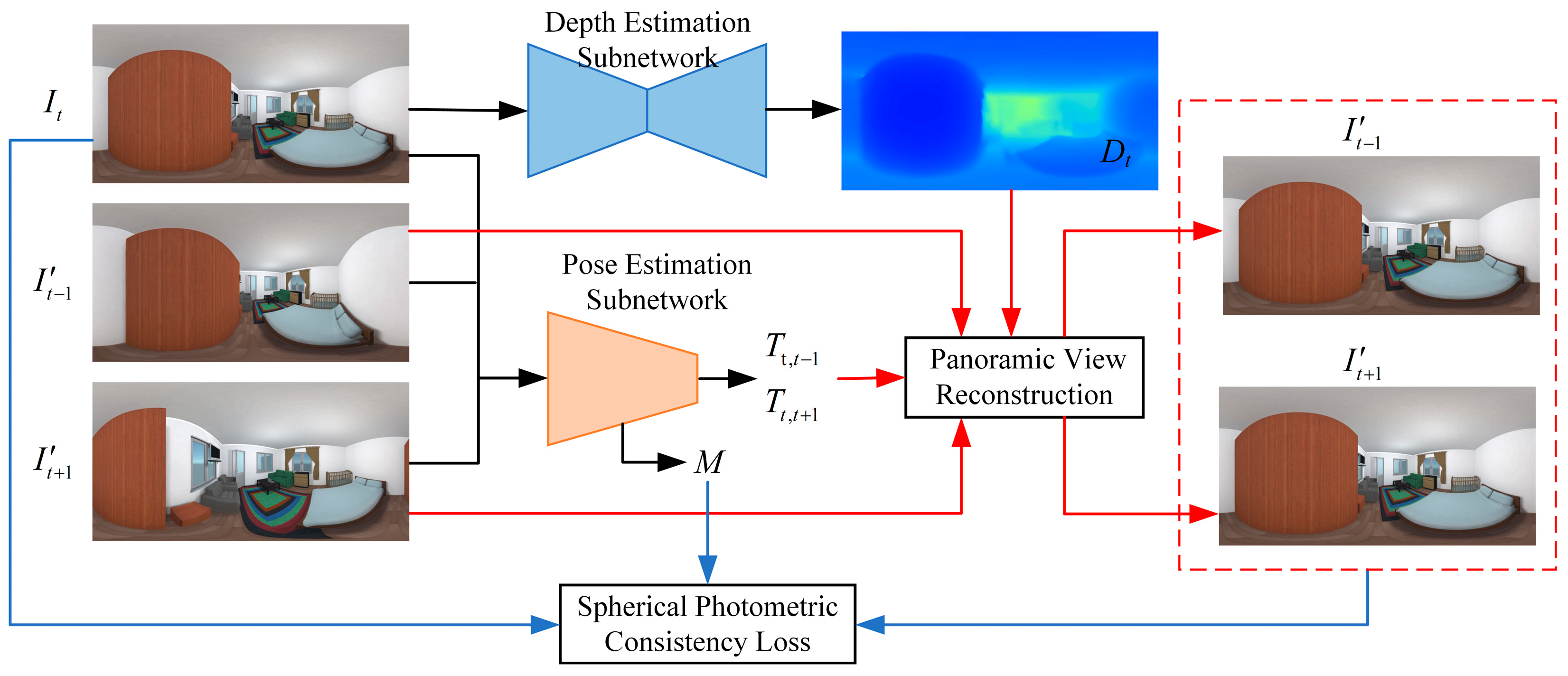
Due to the difficulty in obtaining pose data for panoramic image sequences and the limited availability of public datasets, a panoramic camera pose estimation model based on unsupervised deep learning is proposed to reduce the training complexity and overcome the dependency on pose labels, while fully leveraging panoramic sequences for training, as shown in Figure 1. To enable unsupervised learning through a closed-loop constraint, the model includes not only a pose estimation sub-network but also introduces a depth estimation sub-network. The depth sub-network predicts dense panoramic depth maps, which, together with the pose information estimated by the pose sub-network, are used to reconstruct panoramic views. The reconstructed panoramic image serves as a supervision signal, and a spherical photometric consistency loss between the reconstructed and input panoramas is constructed to enable the joint unsupervised training of both sub-networks.
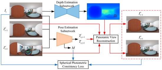
Figure 1.
The input to the panoramic camera pose estimation model consists of three temporally consecutive panoramic images, , , and . Among them, the image is fed into the depth estimation sub-network to produce the corresponding depth map . The three images , , and are concatenated along the channel dimension and input to the pose estimation sub-network, which outputs the relative camera poses and between the central frame and its neighbors, as well as the occlusion mask . Using the view synthesis module, the images and , predicted depth map , and relative poses and are used to reconstruct the corresponding panoramic views and , which serve as supervisory signals during training. The occlusion mask is incorporated to compute the spherical photometric consistency loss between the reconstructed panoramic images and and the input image , thereby enabling joint training of the depth and pose estimation sub-networks over the panoramic image sequence. Although these two sub-networks are trained jointly, they can be used independently during inference.
3.2. Panoramic Depth Estimation Sub-Network
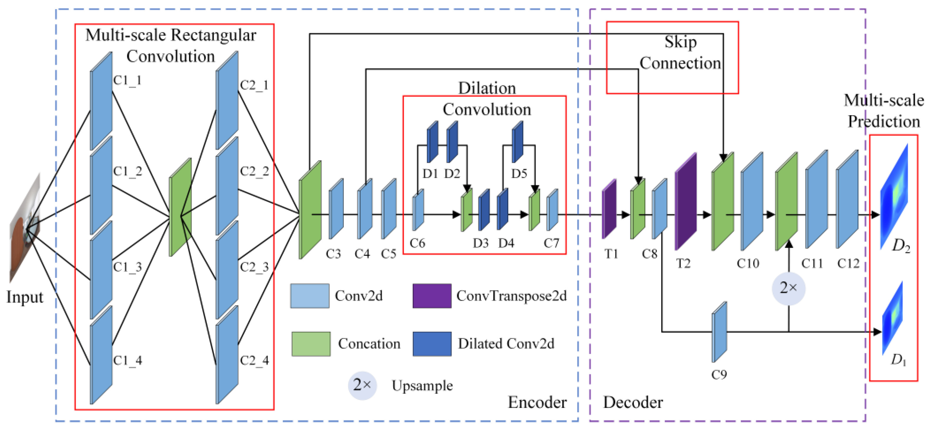
Panoramic depth estimation is a key component in enabling unsupervised panoramic camera pose estimation. Considering the real-time requirements of 3D tracking and registration in augmented reality systems, this chapter proposes a lightweight panoramic depth estimation sub-network tailored for panoramic camera pose estimation. As illustrated in Figure 2 (where C denotes 2D convolution, D denotes dilated convolution, T denotes transposed convolution, and 2× represents upsampling), the network adopts an encoder–decoder architecture with skip connections. The sub-network consists of an encoder, a decoder, and skip connections between them. It takes a single equirectangular panoramic image as input and outputs dense panoramic depth maps at two different scales. The encoder extracts image features using multi-scale rectangular convolution modules, dilated convolutions, and standard convolutional operations. The decoder reconstructs multi-scale depth maps from the encoded features through transposed convolutions and other upsampling techniques, thus achieving the transformation from pixel-level image information to depth information. Meanwhile, skip connections integrate shallow detail features from the encoder with deep semantic features in the decoder, enhancing the network’s robustness and preserving fine-grained details from the input image, thereby producing depth maps with rich structural information.
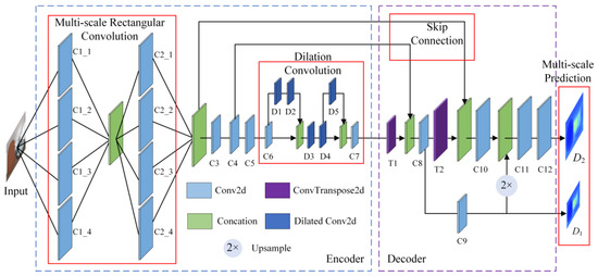
Figure 2.
Panoramic depth estimation sub-network architecture.
Encoder: The encoder mainly consists of multi-scale rectangular convolution modules, dilated convolution modules, and convolutional downsampling operations. The output feature dimensions and corresponding hyperparameters are summarized in Table 1. The hyperparameters of the convolutional operations include kernel size, stride, padding, and dilation rate. The output feature dimensions are represented as channel × height × width.

Table 1.
Output shapes and hyperparameters of encoder operations.
Equirectangular panoramic images typically suffer from significant distortions, especially in the polar regions. While conventional square convolutional filters are effective at extracting features from undistorted perspective images, they are less effective when applied to distorted panoramic images. To address this issue, a multi-scale rectangular convolution module is introduced to mitigate the impact of distortion. According to [28], we employ only two layers of rectangular convolution filters; this design effectively addresses the distortion in ERP images. The most severe geometric distortions occur near the poles and primarily affect low-level features such as edges. By applying distortion-aware filters early, we compensate for these effects before deeper semantic features are extracted. Each rectangular filter block uses multiple aspect ratios with approximately constant area, enabling adaptive feature extraction across image rows. Combined with later dilated convolutions and limited downsampling, which provide large receptive fields, two such layers are sufficient to model the spatially varying distortions without further overhead.
Given the varying degrees of distortion across different regions of a panoramic image, each layer of the multi-scale rectangular convolution module adopts four rectangular convolution filters with different aspect ratios to extract features, thereby reducing the impact of distortion on feature extraction. Since shallow features are helpful for the decoder to reconstruct meaningful representations, a skip connection is introduced after the second layer of the rectangular convolution module. The shallow features are concatenated and passed to the decoder to enhance its feature decoding capability.
To improve computational efficiency, the encoder performs only two downsampling operations on the input image, instead of applying multiple downsampling steps and stacking a large number of convolutional filters. This reduces the number of parameters and makes the network more lightweight. The shallow features obtained after the first downsampling are also passed to the decoder via skip connections, further enhancing the decoder’s ability to interpret features.
However, with only two downsampling stages, the network struggles to capture deep, high-level features from the input image. To compensate for this, a dilated convolution module is introduced to enlarge the receptive field and better extract global contextual information from the image. Furthermore, to enhance the representational capacity of features, the dilated convolution is combined with skip connections, and 1 × 1 convolution filters (D3 and C7) are used to fuse shallow and deep features. In addition, all convolution operations are followed by the ELU activation function to improve the network’s ability to model nonlinear representations.
Decoder: The decoder consists of transposed convolution, upsampling, skip connections, and depth prediction operations. The output feature dimensions and corresponding hyperparameters of each operation are listed in Table 2. To match the two downsampling operations performed by the encoder, the decoder utilizes two transposed convolutions for upsampling. First, a transposed convolution (T1) is applied to upsample the deep features extracted by the encoder. To enhance feature reconstruction, the upsampled features are concatenated with the shallow features of the same spatial resolution passed from the encoder via skip connections. Two large-kernel convolutional layers (C8 and C9) are then applied to the concatenated features to perform depth estimation, generating a coarse depth map at half the input resolution. The feature map produced by the first large-kernel convolution (C8) undergoes a second upsampling via transposed convolution (T2) and is again concatenated with the corresponding shallow features from the encoder. The resulting features are further processed using another large-kernel convolution (C10), while the coarse depth map is simultaneously upsampled using nearest-neighbor interpolation. These two sources of feature information are fused to enhance the quality of the final fine-grained depth prediction. Specifically, two small-kernel convolutional layers (C11 and C12) are employed to fuse the concatenated features and produce a high-resolution depth map with the same resolution as the input image. In addition, except for the convolutional layers used for depth prediction (C9 and C12), all other convolutional operations in the decoder are followed by the ELU activation function to enhance the non-linear representational capacity and stability of the network.
Table 2.
Output shapes and hyperparameters of decoder operations.
Since the depth values estimated by the depth estimation sub-network are relative and the depth range in panoramic images is typically wide, the estimated depth values are normalized to a reasonable range to facilitate more effective utilization of the depth information. The estimated depth values are normalized as follows (Equation (1)):
where denotes the output of the sub-network predicting depth, is the Sigmoid activation function, and are hyperparameters. is the normalized depth map, and represents different resolutions, where s = 1 indicates half-resolution, and s = 2 indicates full-resolution. In the experiment, and are used to normalize the depth values within a range of 10 m.
3.3. Panoramic Pose Estimation Sub-Network
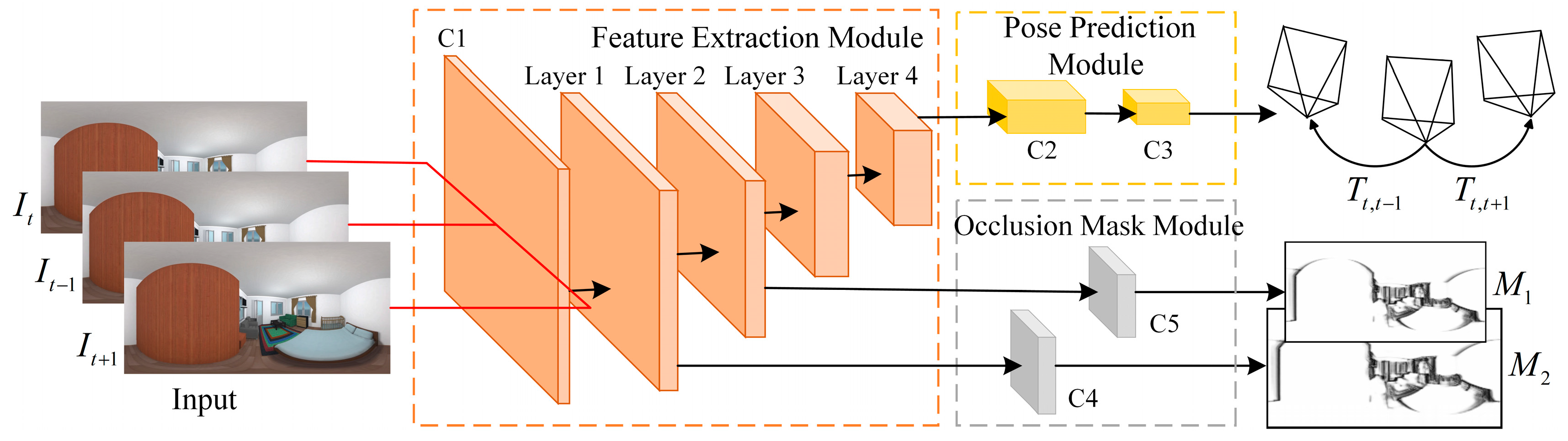
The relative camera pose estimation network is designed based on an encoder–decoder sub-network, aiming to estimate the relative poses between neighboring frames as well as to compute occlusion masks between adjacent images. The network comprises a feature extraction module, a pose prediction module, and an occlusion mask module group, as illustrated in Figure 3. The entire image sequence is provided as input, and the network is trained to predict the global frame , along with the relative poses and between neighboring frames and , as well as multi-scale occlusion masks .
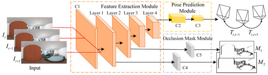
Figure 3.
Panoramic pose estimation sub-network architecture.
To ensure a lightweight architecture, the pose estimation sub-network adopts an encoder design. The feature extraction module is built upon ResNet18 [29], consisting of one convolutional layer followed by four residual blocks. Given that three consecutive frames are input simultaneously, the number of input channels is set to 9, allowing for the extraction of shallow features from the input images. The four residual blocks capture features at multiple scales, with each block composed of standard residual units. Each residual unit contains two 3 × 3 convolutional layers and a residual skip connection from input to output. The pose prediction module comprises five convolutional layers and one global average pooling layer. It outputs two 6-DoF relative poses, , for the three input images, where each pose vector includes translation and rotation parameters. Rotations are represented using Euler angles. The occlusion mask module utilizes intermediate features at two different resolutions from the feature extraction module. These are passed through two convolutional layers to produce occlusion masks and at different scales, which represent the occluded regions resulting from camera motion between neighboring frames.
The camera pose estimation sub-network exhibits a certain degree of robustness to dynamic scene motions. This is attributed to the use of an unsupervised learning approach based on view reconstruction, which relies on the following assumptions: (1) All objects in the scene are static, and only the camera is moving, i.e., the scene is rigid, and the appearance changes between adjacent frames are primarily caused by camera motion. (2) Objects are assumed to remain visible across adjacent frames, without being occluded or leaving the field of view due to either camera motion or object motion. (3) The illumination of the same object should remain consistent across adjacent frames, implying that no strong reflections are present and all surfaces exhibit Lambertian reflectance.
However, in real-world environments, moving objects and dynamic occlusions are common, and many surfaces exhibit reflective properties. These issues violate the illumination-invariance assumption critical to pose estimation tasks, thus impairing the network’s ability to predict accurate poses. To address these challenges, the camera pose estimation sub-network incorporates an occlusion mask module, designed to generate multi-scale occlusion masks that mitigate the effects of such violations within the image sequence. The occlusion mask module consists of convolutional layers followed by a Sigmoid activation function. Since the panoramic depth estimation sub-network predicts depth maps at two different scales, corresponding reconstructed images are generated via the view reconstruction module. Occlusion masks are applied to these reconstructed images when computing the photometric loss, and it is therefore essential to ensure resolution consistency between the occlusion masks and the reconstructed images. Consequently, the occlusion masks are estimated from feature maps output by the first two residual blocks of the feature extraction module, matching the respective scales. The occlusion mask is a grayscale image with values ranging from 0 to 1, where pixels with intermediate intensity represent regions occluded due to object motion, helping to reduce the adverse impact of occlusion on accurate pose estimation. The output feature dimensions and hyperparameters for each module within the camera pose estimation sub-network are summarized in Table 3.
Table 3.
Output dimensions and hyperparameters of the pose estimation sub-network.
3.4. Panoramic View Reconstruction
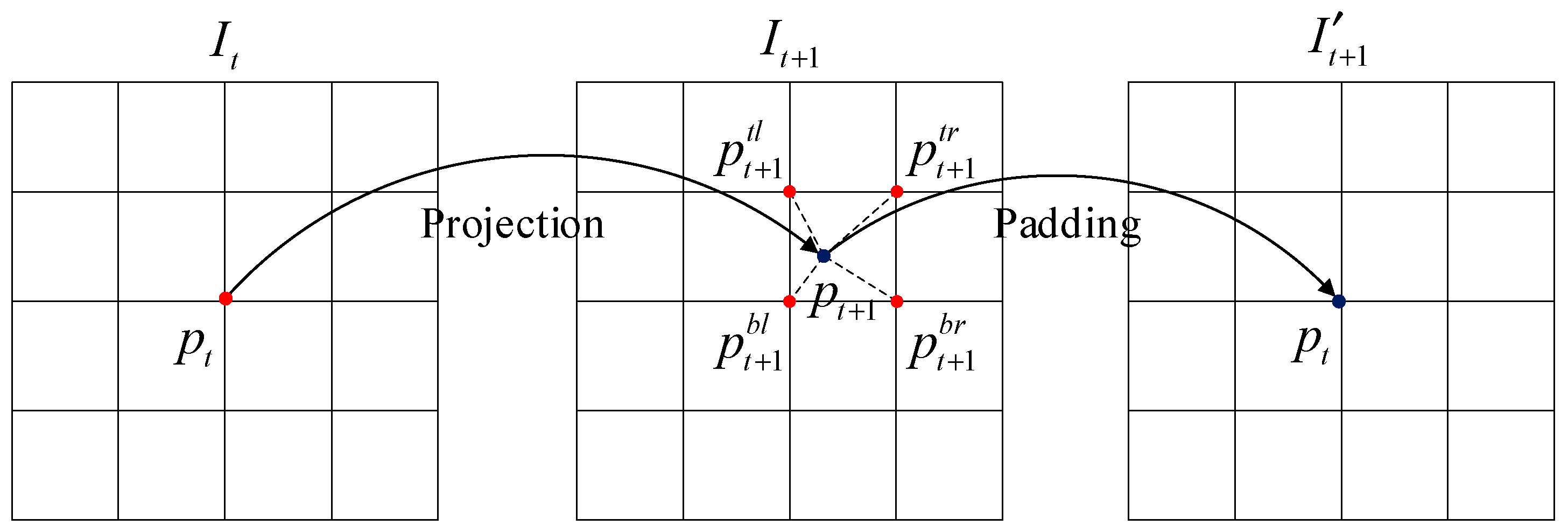
Panoramic view reconstruction synthesizes novel views of the scene by using the input panoramic image and its corresponding depth map, combined with camera poses from different viewpoints. This process involves two main steps: pixel coordinate projection and pixel value interpolation filling, as illustrated in Figure 4.
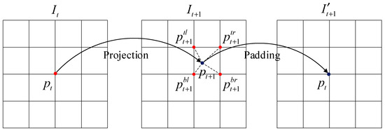
Figure 4.
Illustration of the panoramic view reconstruction process, which involves pixel coordinate projection and value interpolation based on depth and camera pose information.
During the motion of the panoramic camera, suppose the panoramic image captured at time is denoted as , with its corresponding depth map , and the image captured at time is denoted as . The relative camera pose from time to is represented as . Through pixel coordinate projection, any pixel in image is projected to a corresponding pixel in image . Then, via pixel value interpolation, the pixel value at in image is used to fill the corresponding location in image , generating a synthesized view , where the pixel value at corresponds to that of .
In the process of pixel coordinate mapping, the projected pixel in image may fall into one of the following three cases: if the image coordinates of fall outside the valid range of image , the corresponding pixel value in the reconstructed image is set to zero; if the image coordinates of lie within the valid image range and are integers, the corresponding pixel value in the reconstructed image is directly assigned as = ; if the image coordinates of are within the valid image range but contain fractional values, the exact pixel value at in image cannot be directly retrieved. In this case, bilinear interpolation is employed using the pixel values of the four neighboring pixels—top left , top right , bottom left , and bottom right . The interpolated pixel value is computed as (Equation (2)):
where denotes one of the four neighboring pixels around , and is the corresponding pixel value in image . Let and represent the horizontal and vertical distances from to its top-left neighbor , respectively. Then, the interpolation weights for and are given by , , , and , which meet the condition . According to Equation (2), the final pixel value is obtained by bilinear interpolation of the top left, top right, bottom left, and bottom right neighbors of , and the result is used to fill the corresponding pixel in the synthesized view .
3.5. Loss Function
During camera pose estimation, it is assumed that the illumination of the same scene point remains constant across different viewpoints, due to the predominantly diffuse nature of surfaces in real-world environments. Based on this assumption, to enable unsupervised learning across the entire network, a spherical photometric consistency loss is employed as a supervisory signal. This loss is computed using the input image, its corresponding reconstructed images, and occlusion masks. Let denote a pixel at the same coordinate in the input image , the reconstructed images , , and the occlusion mask . The spherical photometric consistency loss is (Equation (3)):
where , as defined in Equation (1), represents different resolution levels, and denotes the set of all pixel coordinates in the image. The term represents the sum of absolute photometric differences between the input image and its forward and backward reconstructed views (Equation (4)):
where and denote the images reconstructed at scale from the -th and -th frames, respectively, targeting the current frame.
In addition to the spherical photometric consistency loss, two regularization terms are introduced to constrain the predicted occlusion mask and depth map. To prevent the predicted occlusion mask from collapsing to zero during training, a binary cross-entropy loss is applied to multi-scale occlusion masks (Equation (5)):
As can be seen from Equation (5), the regularization term imposes a larger penalty when the occlusion mask values are small. To reduce noise in the predicted depth map, a smoothness regularization term is also applied (Equation (6)):
where and denote the horizontal and vertical gradients of the predicted depth map , respectively. By linearly combining the above three loss terms, the final loss function is defined as (Equation (7)):
where and are hyperparameters that balance the occlusion mask regularization and depth smoothness regularization, respectively.
4. Experiments
The experiments were conducted on a high-performance computing platform equipped with an Intel Xeon(R) CPU, 128 GB of RAM, and an NVIDIA RTX 3090 GPU with 24 GB of VRAM. The software environment consisted of the 64-bit Ubuntu 20.04 LTS operating system, Python 3.8 as the programming language, and PyTorch 1.11 as the deep learning framework. GPU acceleration was enabled using CUDA 11.1 and cuDNN 8.0 libraries.
4.1. Experimental Settings
Datasets: The experiments in this chapter were conducted on the publicly available synthetic panoramic video dataset, PanoSUNCG [18]. This dataset is constructed from 103 indoor scenes selected from the SUNCG dataset [30], where five virtual panoramic camera trajectories are defined for each scene. RGB-D panoramic video sequences and corresponding camera pose annotations are rendered using the Unity engine, with an original image resolution of 512 × 1024. Among these scenes, 80 are used for training and 23 for testing. To improve computational efficiency during camera pose estimation model training, all images are downsampled to a resolution of 256 × 512 for both training and testing phases.
Training details: During network training, the Adam optimizer [31] was employed with default momentum parameters and . The batch size was set to 8, and the initial learning rate was fixed at 0.0001. The scene depth estimation sub-network was initialized using Xavier initialization [32], while the camera pose estimation sub-network was initialized with pre-trained weights from the ImageNet dataset [33]. Following the setup in [18], the hyperparameters of the loss function were set to and , respectively. The entire network was trained for 100 epochs, which took approximately two days to complete.
Evaluation metrics: For the evaluation of panoramic depth estimation, standard error and accuracy metrics proposed in depth estimation literature [34] were adopted. Error metrics include the Mean Relative Error (MRE), Mean Absolute Error (MAE), Root Mean Square Error (RMSE), and Root Mean Square Log Error (RMSElog), which measure the discrepancy between the predicted depth and the ground truth depth . Accuracy metrics are defined as the percentage of pixels for which the ratio between the predicted depth and ground truth depth is below a certain threshold, specifically < 1.25, < 1.252, and < 1.253. The evaluation metrics are computed as follows:
where denotes the number of valid depth values in the ground truth depth map . Additionally, since the entire network is trained in an unsupervised manner, the predicted depth maps lack an absolute scale. Therefore, prior to evaluation, the predicted depth is aligned with the ground truth depth using median scaling, defined as:
where the function is used to compute the median of valid depth values in the depth map, and denotes the predicted depth map after median scaling.
For camera pose estimation, the Relative Pose Error (RPE) [35] is adopted as the evaluation metric. RPE measures the accuracy of the relative motion between two camera poses separated by a fixed time interval . The relative pose error for the -th frame is defined as:
where and denote the ground truth and estimated camera poses, respectively. Given a sequence of camera frames, a total of relative pose errors can be computed. The RMSE of all relative pose errors is then calculated. The translation and rotation components of the RPE are measured as follows:
where and denote the translation error (in meters) and rotation error (in degrees), respectively. In the experiment, is used to evaluate the relative pose error between consecutive camera frames.
4.2. Comparison Results
The proposed method is compared with the traditional approach, OpenVSLAM [13], and two other unsupervised methods, 360-SelfNet [18] and BiFuse++ [22]. The comparison includes both the estimation results of scene depth and the estimation accuracy of camera pose parameters.
Comparison of Scene Depth Estimation Results. To verify the effectiveness of the proposed method in scene depth estimation, the model is evaluated on the test set derived from the PanoSUNCG dataset, which consists of panoramic image sequences from 23 different scenes. Since the traditional method, OpenVSLAM, reconstructs a sparse map based on feature point matching, it can only generate sparse point clouds. In contrast, the proposed method, along with 360-SelfNet and BiFuse++, can generate dense depth maps. Therefore, a direct comparison with OpenVSLAM in terms of scene depth information is not applicable. Figure 5 presents the visual comparison of depth estimation results across different methods. Each row corresponds to the same input image, while each column shows the depth maps estimated by 360-SelfNet, BiFuse++, and the proposed method, as well as the ground truth depth map. As shown in Figure 5, noticeable differences can be observed among the results of different depth estimation methods. The 360-SelfNet method estimates depth on cubemap panoramic images, which leads to discontinuities in the generated depth maps. In contrast, BiFuse++ addresses image distortion by fusing features from both cubemap and equirectangular panoramas and directly predicts depth on equirectangular panoramas, resulting in improved estimation quality. The proposed method employs rectangular convolution filters at multiple scales to handle the distortion in equirectangular panoramic images, achieving depth estimation results comparable to BiFuse++ and significantly better than 360-SelfNet.
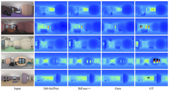
Figure 5.
Comparison of panoramic depth estimation visualization results.
To comprehensively validate the effectiveness of panoramic depth estimation, the experiment adopts the four error evaluation metrics and three accuracy evaluation metrics described in Section 4.1 as quantitative indicators of prediction accuracy. Lower values in error metrics indicate more precise estimations, while higher values in accuracy metrics represent more reliable results.
From Table 4, it can be observed that the BiFuse++ method achieves the best overall performance, while the proposed method yields the second-best results. This is because BiFuse++ employs a depth estimation network that fuses features from both equirectangular and cubemap panoramas, providing a more effective solution to panoramic image distortion than the proposed method. Consequently, BiFuse++ outperforms our method in terms of accuracy. In contrast, 360-SelfNet estimates depth based on cubemap panoramas using a network originally designed for perspective images. While this approach avoids handling distortion in equirectangular panoramas, it suffers from discontinuities at the cube face boundaries, which negatively impact the accuracy of the estimated depth maps. Comparatively, the proposed method applies multi-scale rectangular convolution modules to address distortion, leverages dilated convolutions to expand the receptive field, and directly estimates depth on equirectangular panoramic images. These strategies enable our method to outperform 360-SelfNet in depth prediction accuracy.
Table 4.
Quantitative comparison of panoramic depth estimation results across different methods. ↓ indicates that lower is better; ↑ indicates that higher is better. Bold values denote the best performance, and underlined values represent the second-best results.
Comparison of Camera Pose Estimation Results. To thoroughly validate the effectiveness of panoramic camera pose estimation, the experiment adopts the Relative Pose Error (RPE) as the evaluation metric. As shown in Table 5, the traditional method, OpenVSLAM, achieves the best results (bolded), while the deep learning-based BiFuse++ method ranks second (underlined). The proposed method yields PRE-R and RPE-T values that are 0.13° and 0.001 m higher than those of BiFuse++, but 0.10° and 0.002 m lower than those of 360-SelfNet, respectively. Overall, the proposed method achieves competitive results. Moreover, the performance of the camera pose estimation aligns with the corresponding depth estimation results.
Table 5.
Quantitative comparison of panoramic pose estimation results across different methods. ↓ indicates that lower is better. Bold values denote the best performance, and underlined values represent the second-best results.
4.3. Ablation Study
To investigate the impact of different types of supervision signals on pose estimation performance, ablation studies were conducted on the pose estimation sub-network using supervised learning strategies. The specific ablation experiments are as follows:
Fully Unsupervised Training: The network was trained without any labels by leveraging spherical photometric consistency loss to estimate camera motion.
Fully Unsupervised Training without M: To investigate the role of occlusion handling in the pose estimation process, we remove the occlusion mask module from the pose sub-network. The model is still trained under the same fully unsupervised setting, using only the spherical photometric consistency loss for supervision.
Fully Unsupervised Training without D1: To assess the contribution of multi-scale depth features, we remove the low-resolution depth branch and retain only the full-resolution depth map for supervision. The network remains fully unsupervised and continues to rely solely on the spherical photometric consistency loss.
Supervised with Pose Labels: To enhance the supervision signals, pose labels were introduced as supervision, and an L1 loss was used to guide training. This strategy enables the network to better learn pose information, thereby improving the accuracy of pose estimation.
Noisy Pose Ground-Truth Supervision: Considering that pose estimation in real-world scenarios may be prone to drift, pose noise was simulated by adding Gaussian noise with a mean of 0 and a standard deviation of 0.1 to the ground-truth pose. This mimics the accumulation of pose estimation errors in real-world applications. To mitigate this drift effect, pose labels and the L1 loss were also used for supervised training, allowing the network to gradually reduce pose deviation errors.
Pose Estimator Only Training: The pose estimation sub-network was trained independently, supervised by calculating the L1 loss between the estimated poses and the ground-truth labels.
As shown in Table 6, training the network with pose ground-truth significantly improves the accuracy of the pose estimation.
Table 6.
Ablation results of panoramic pose estimation. ↓ indicates that lower is better.
4.4. Complexity Comparison
Table 7 compares the algorithmic complexity of different models, focusing on the number of parameters and computation time. The test data consists of five randomly selected scenes from the test set, each containing 5000 images with a resolution of 256 × 512. For the traditional method, OpenVSLAM, the evaluation was conducted on an Intel Xeon(R) CPU, while for deep learning-based methods, an NVIDIA RTX 3090 GPU was used. The computation time refers to the average inference time across all test data.
Table 7.
Performance comparison. Bold values denote the best performance, and underlined values represent the second-best results.
As shown in Table 7, the traditional method, OpenVSLAM, estimates camera poses using handcrafted features and does not involve any learnable parameters, resulting in an inference time of 45.52 ms. 360-SelfNet estimates depth and camera poses based on cubemap panoramic images, with a model size of 33.32 M parameters and an inference time of 28.29 ms. BiFuse++ employs a depth estimation network composed of two ResNet34 encoders and four fusion modules, along with a pose estimation network based on a ResNet18 backbone. This results in a total of 60.88 M parameters and an inference time of 38.11 ms. The method proposed in this chapter designs lightweight sub-networks for both scene depth estimation and camera pose estimation, achieving a total model size of 20.26 M parameters and an inference time of 24.65 ms. Compared with 360-SelfNet and BiFuse++, the proposed method reduces the number of parameters by 39.20% and 66.72%, respectively, and decreases inference time by 12.87% and 35.32%. Therefore, the proposed approach achieves relatively high accuracy with significantly lower model complexity.
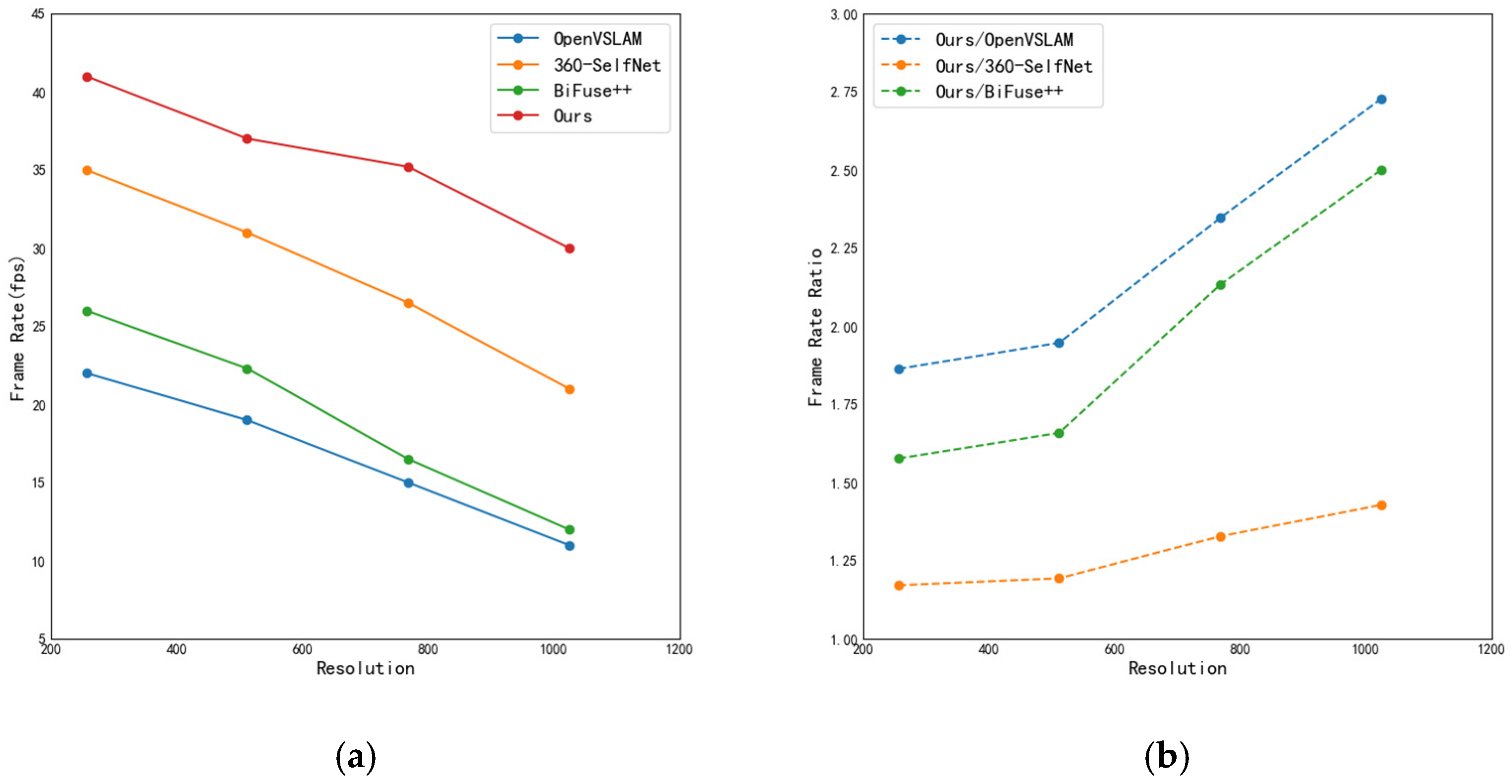
Figure 6 illustrates the impact of image resolution on model performance. In Figure 6a, the horizontal axis represents the number of pixels in the vertical direction of the equirectangular panoramic image, corresponding to resolutions of 256 × 512, 512 × 1024, 768 × 1536, and 1024 × 2048. The vertical axis denotes the number of images processed per second by the model, i.e., the frame rate (Frames Per Second, FPS). In Figure 6b, the vertical axis represents the ratio of FPS between the proposed method and other approaches. As shown in Figure 6a, the FPS gap increases with rising image resolution. Figure 6b demonstrates that the FPS ratio consistently grows as the resolution increases, indicating that the performance of the proposed method degrades more slowly compared to other methods. Therefore, when performing pose estimation on high-resolution panoramic images, the proposed method can significantly reduce computational cost.
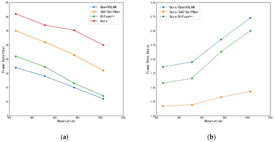
Figure 6.
The impact of image resolution on model efficiency. (a) Relationship between resolution and frame rate. (b) Relationship between resolution and the resolution-to-frame rate ratio.
4.5. Limitations Analysis
In this chapter, a lightweight camera pose estimation model was designed to ensure the real-time performance of panoramic camera tracking and registration. However, the model still exhibits certain limitations. First, the depth estimation sub-network performs only two downsampling operations on the input image. Although this design contributes to the lightweight nature of the model, it also limits the network’s ability to capture comprehensive global contextual information, thereby affecting the accuracy of depth estimation and ultimately reducing the precision of pose estimation. Second, the model processes image data at a resolution of 256 × 512. When applied to higher-resolution panoramic images, the accuracy of the predicted depth maps may degrade significantly, which restricts the model’s overall performance and application scope. To overcome these limitations, we consider incorporating model distillation techniques. For instance, a larger teacher model with stronger representation capabilities can be used to guide the training of our lightweight panoramic pose estimation network. Such approaches may help retain high-resolution performance while maintaining inference efficiency, and this will be an important direction for our future work.
5. Conclusions
In this paper, we propose an unsupervised deep learning-based model for panoramic camera pose estimation. To address the issues of inefficiency, label scarcity, and complex relative motion in panoramic camera pose estimation, a lightweight architecture is designed, comprising a depth estimation sub-network and a camera pose estimation sub-network. The depth estimation sub-network incorporates several lightweight modules and operations. Specifically, a multi-scale rectangular convolution module is employed to address distortion issues commonly found in panoramic images. A dilated convolution module is used to enlarge the receptive field of the network, while skip connections are introduced to fuse shallow detail features with deep semantic features. Additionally, multi-scale prediction is utilized to improve the accuracy of depth estimation. The camera pose estimation sub-network leverages a pose estimation module and an occlusion mask module to infer the relative camera motion and occlusion masks between adjacent image pairs from a shared encoder, without using a decoder, thereby further reducing the computational load and making the network more lightweight. To enable joint training of the two sub-networks, a spherical photometric consistency loss is designed based on panoramic view reconstruction. Experimental results demonstrate that the proposed method achieves a good balance between accuracy and efficiency on the synthetic panoramic sequence dataset.
Author Contributions
Conceptualization, C.X.; methodology, G.L.; software, G.L.; validation, Y.B. (Yuzhuo Bai); formal analysis, Y.B. (Yuzhuo Bai); investigation, C.H.; resources, Y.B. (Ye Bai); data curation, Z.C.; writing—original draft preparation, G.L.; writing—review and editing, Y.B. (Ye Bai) and C.H.; visualization, Z.C.; supervision, Y.B. (Ye Bai) and C.H.; project administration, C.X.; funding acquisition, C.X. All authors have read and agreed to the published version of the manuscript.
Funding
This research was funded by the Natural Science Foundation of Jilin of China, grant number 20250102241JC.
Institutional Review Board Statement
Not applicable.
Informed Consent Statement
Not applicable.
Data Availability Statement
Restrictions apply to the availability of these data. Data were obtained from the authors of the paper “Self-Supervised Learning of Depth and Camera Motion from 360 Videos” (Wang et al., ACCV 2018 [18]), and are available from the authors with the permission of the original authors.
Conflicts of Interest
The authors declare no conflicts of interest.
References
- Kato, H.; Billinghurst, M. Marker Tracking and HMD Calibration for a Video-Based Augmented Reality Conferencing System. In Proceedings of the 2nd IEEE and ACM International Workshop on Augmented Reality (IWAR’99), San Francisco, CA, USA, 20–21 October 1999; IEEE: San Francisco, CA, USA, 1999; pp. 85–94. [Google Scholar]
- Wagner, D.; Schmalstieg, D.; Bischof, H. Multiple target detection and tracking with guaranteed framerates on mobile phones. In Proceedings of the 8th IEEE International Symposium on Mixed and Augmented Reality, Orlando, FL, USA, 19–22 October 2009; pp. 57–64. [Google Scholar]
- Klein, G.; Murray, D. Parallel tracking and mapping for small AR workspaces. In Proceedings of the 6th IEEE and ACM International Symposium on Mixed and Augmented Reality, Nara, Japan, 13–16 November 2007; pp. 225–234. [Google Scholar]
- Mur-Artal, R.; Tardós, J.D. ORB-SLAM2: An open-source SLAM system for monocular, stereo, and RGB-D cameras. IEEE Trans. Robot. 2017, 33, 1255–1262. [Google Scholar] [CrossRef]
- Newcombe, R.A.; Lovegrove, S.J.; Davison, A.J. DTAM: Dense tracking and mapping in real-time. In Proceedings of the 2011 International Conference on Computer Vision (ICCV), Barcelona, Spain, 6–13 November 2011; pp. 2320–2327. [Google Scholar]
- Engel, J.; Schöps, T.; Cremers, D. LSD-SLAM: Large-scale direct monocular SLAM. In Proceedings of the European Conference on Computer Vision (ECCV), Zurich, Switzerland, 6–12 September 2014; pp. 834–849. [Google Scholar]
- Engel, J.; Koltun, V.; Cremers, D. Direct sparse odometry. IEEE Trans. Pattern Anal. Mach. Intell. 2017, 40, 611–625. [Google Scholar] [CrossRef] [PubMed]
- Forster, C.; Pizzoli, M.; Scaramuzza, D. SVO: Fast semi-direct monocular visual odometry. In Proceedings of the 2014 IEEE International Conference on Robotics and Automation (ICRA), Hong Kong, China, 31 May–7 June 2014; pp. 15–22. [Google Scholar]
- Matsuki, H.; Von Stumberg, L.; Usenko, V.; Stückler, J.; Cremers, D. Omnidirectional DSO: Direct Sparse Odometry with Fisheye Cameras. IEEE Robot. Autom. Lett. 2018, 3, 3693–3700. [Google Scholar] [CrossRef]
- Seok, H.; Lim, J. ROVO: Robust Omnidirectional Visual Odometry for Wide-Baseline Wide-FoV Camera Systems. In Proceedings of the 2019 International Conference on Robotics and Automation (ICRA), Montreal, QC, Canada, 20–24 May 2019; pp. 6344–6350. [Google Scholar]
- Ji, S.; Qin, Z.; Shan, J.; Lu, M. Panoramic SLAM from a Multiple Fisheye Camera Rig. ISPRS J. Photogramm. Remote Sens. 2020, 159, 169–183. [Google Scholar] [CrossRef]
- Huang, H.; Yeung, S.-K. 360VO: Visual Odometry Using a Single 360 Camera. In Proceedings of the 2022 International Conference on Robotics and Automation (ICRA), Philadelphia, PA, USA, 23–27 May 2022; pp. 5594–5600. [Google Scholar]
- Sumikura, S.; Shibuya, M.; Sakurada, K. OpenVSLAM: A Versatile Visual SLAM Framework. In Proceedings of the 27th ACM International Conference on Multimedia, Nice, France, 21–25 October 2019; pp. 2292–2295. [Google Scholar]
- Kendall, A.; Grimes, M.; Cipolla, R. Posenet: A Convolutional Network for Real-Time 6-DoF Camera Relocalization. In Proceedings of the IEEE International Conference on Computer Vision, Santiago, Chile, 7–13 December 2015; pp. 2938–2946. [Google Scholar]
- Wang, S.; Clark, R.; Wen, H.; Trigoni, N. DeepVO: Towards End-to-End Visual Odometry with Deep Recurrent Convolutional Neural Networks. In Proceedings of the 2017 IEEE International Conference on Robotics and Automation (ICRA), Singapore, 29 May–3 June 2017; pp. 2043–2050. [Google Scholar]
- Zhou, T.; Brown, M.; Snavely, N.; Lowe, D.G. Unsupervised Learning of Depth and Ego-Motion from Video. In Proceedings of the IEEE Conference on Computer Vision and Pattern Recognition (CVPR), Honolulu, HI, USA, 21–26 July 2017; pp. 1851–1858. [Google Scholar]
- Yin, Z.; Shi, J. GeoNet: Unsupervised Learning of Dense Depth, Optical Flow and Camera Pose. In Proceedings of the IEEE Conference on Computer Vision and Pattern Recognition (CVPR), Salt Lake City, UT, USA, 18–22 June 2018; pp. 1983–1992. [Google Scholar]
- Wang, F.-E.; Hu, H.-N.; Cheng, H.-T.; Lin, J.-T.; Yang, S.-T.; Shih, M.-L.; Chu, H.-K.; Sun, M. Self-Supervised Learning of Depth and Camera Motion from 360 Videos. In Proceedings of the Asian Conference on Computer Vision, Perth, Australia, 2–6 December 2018; Springer: Cham, Switzerland, 2018; pp. 53–68. [Google Scholar]
- Sharma, A.; Ventura, J. Unsupervised Learning of Depth and Ego-Motion from Cylindrical Panoramic Video. In Proceedings of the 2019 IEEE International Conference on Artificial Intelligence and Virtual Reality (AIVR), San Diego, CA, USA, 9–11 December 2019; p. 139. [Google Scholar]
- Liu, M.; Wang, S.; Guo, Y.; He, Y.; Xue, H. Pano-SfMLearner: Self-Supervised Multi-Task Learning of Depth and Semantics in Panoramic Videos. IEEE Signal Process. Lett. 2021, 28, 832–836. [Google Scholar] [CrossRef]
- Hasegawa, Y.; Ikehata, S.; Aizawa, K. Distortion-Aware Self-Supervised 360° Depth Estimation from a Single Equirectangular Projection Image. arXiv 2022, arXiv:2204.01027. [Google Scholar]
- Wang, F.-E.; Yeh, Y.-H.; Tsai, Y.-H.; Chiu, W.-C.; Sun, M. Bifuse++: Self-Supervised and Efficient Bi-Projection Fusion for 360° Depth Estimation. IEEE Trans. Pattern Anal. Mach. Intell. 2022, 45, 5448–5460. [Google Scholar] [CrossRef] [PubMed]
- Hou, S.; Han, J.; Zhang, Y.; Zhu, Z. Survey of Vision-Based Augmented Reality 3D Registration Technology. J. Syst. Simul. 2019, 31, 2206–2215. [Google Scholar]
- Zhi, H.; Yin, C.; Li, H. Review of Visual Odometry Methods Based on Deep Learning. Comput. Eng. Appl. 2022, 58, 1–15. [Google Scholar]
- Zhang, Z.; Rebecq, H.; Forster, C.; Scaramuzza, D. Benefit of Large Field-of-View Cameras for Visual Odometry. In Proceedings of the 2016 IEEE International Conference on Robotics and Automation (ICRA), Stockholm, Sweden, 16–21 May 2016; pp. 801–808. [Google Scholar]
- Campos, C.; Elvira, R.; Rodríguez, J.J.G.; Montiel, J.M.M.; Tardós, J.D. ORB-SLAM3: An Accurate Open-Source Library for Visual, Visual–Inertial, and Multimap SLAM. IEEE Trans. Robot. 2021, 37, 1874–1890. [Google Scholar] [CrossRef]
- Caruso, D.; Engel, J.; Cremers, D. Large-Scale Direct SLAM for Omnidirectional Cameras. In Proceedings of the 2015 IEEE/RSJ International Conference on Intelligent Robots and Systems (IROS), Hamburg, Germany, 28 September–2 October 2015; pp. 141–148. [Google Scholar]
- Zioulis, N.; Karakottas, A.; Zarpalas, D.; Daras, P. Omnidepth: Dense Depth Estimation for Indoors Spherical Panoramas. In Proceedings of the European Conference on Computer Vision (ECCV), Munich, Germany, 8–14 September 2018; pp. 448–465. [Google Scholar]
- He, K.; Zhang, X.; Ren, S.; Sun, J. Deep Residual Learning for Image Recognition. In Proceedings of the IEEE Conference on Computer Vision and Pattern Recognition (CVPR), Las Vegas, NV, USA, 27–30 June 2016; pp. 770–778. [Google Scholar]
- Song, S.; Yu, F.; Zeng, A.; Chang, A.X.; Savva, M.; Funkhouser, T. Semantic Scene Completion from a Single Depth Image. In Proceedings of the IEEE Conference on Computer Vision and Pattern Recognition (CVPR), Honolulu, HI, USA, 21–26 July 2017; pp. 1746–1754. [Google Scholar]
- Kinga, D.; Ba, J. Adam: A Method for Stochastic Optimization. In Proceedings of the International Conference on Learning Representations (ICLR), San Diego, CA, USA, 7–9 May 2015; Volume 5. [Google Scholar]
- Glorot, X.; Bengio, Y. Understanding the Difficulty of Training Deep Feedforward Neural Networks. In Proceedings of the Thirteenth International Conference on Artificial Intelligence and Statistics (AISTATS), Sardinia, Italy, 13–15 May 2010; pp. 249–256. [Google Scholar]
- Deng, J.; Dong, W.; Socher, R.; Li, L.-J.; Li, K.; Fei-Fei, L. ImageNet: A Large-Scale Hierarchical Image Database. In Proceedings of the 2009 IEEE Conference on Computer Vision and Pattern Recognition (CVPR), Miami, FL, USA, 20–25 June 2009; pp. 248–255. [Google Scholar]
- Eigen, D.; Puhrsch, C.; Fergus, R. Depth Map Prediction from a Single Image Using a Multi-Scale Deep Network. In Proceedings of the Advances in Neural Information Processing Systems (NeurIPS), Montreal, QC, Canada, 8–13 December 2014; Volume 27. [Google Scholar]
- Sturm, J.; Engelhard, N.; Endres, F.; Burgard, W.; Cremers, D. A Benchmark for the Evaluation of RGB-D SLAM Systems. In Proceedings of the 2012 IEEE/RSJ International Conference on Intelligent Robots and Systems (IROS), Vilamoura, Portugal, 7–12 October 2012; pp. 573–580. [Google Scholar]

Disclaimer/Publisher’s Note: The statements, opinions and data contained in all publications are solely those of the individual author(s) and contributor(s) and not of MDPI and/or the editor(s). MDPI and/or the editor(s) disclaim responsibility for any injury to people or property resulting from any ideas, methods, instructions or products referred to in the content. |
© 2025 by the authors. Licensee MDPI, Basel, Switzerland. This article is an open access article distributed under the terms and conditions of the Creative Commons Attribution (CC BY) license (https://creativecommons.org/licenses/by/4.0/).