Abstract
Air quality (AQ) modeling is at the forefront of estimating pollution levels in areas where the spatial representativity is low. Large metropolitan areas in Asia such as Beijing face significant pollution issues due to rapid industrialization and urbanization. AQ nowcasting, especially in dense urban centers like Beijing, is crucial for public health and safety. One of the most popular and accurate modeling methodologies relies on black-box models that fail to explain the phenomena in an interpretable way. This study investigates the performance and interpretability of Explainable AI (XAI) applied with the eXtreme Gradient Boosting (XGBoost) algorithm employing the SHapley Additive exPlanations (SHAP) and the Local Interpretable Model-Agnostic Explanations (LIME) for PM2.5 nowcasting. Using a SHAP-based technique for dimensionality reduction, we identified the features responsible for 95% of the target variance, allowing us to perform an effective feature selection with minimal impact on accuracy. In addition, the findings show that SHAP and LIME supported orthogonal insights: SHAP provided a view of the model performance at a high level, identifying interaction effects that are often overlooked using gain-based metrics such as feature importance; while LIME presented an enhanced overlook by justifying its local explanation, providing low-bias estimates of the environmental data values that affect predictions. Our evaluation set included 12 monitoring stations using temporal split methods with or without lagged-feature engineering approaches. Moreover, the evaluation showed that models retained a substantial degree of predictive power (R2 > 0.93) even in a reduced complexity size. The findings provide evidence for deploying interpretable and performant AQ modeling tools where policy interventions cannot solely depend on predictive analytics tools. Overall, the findings demonstrate the large potential of directly incorporating explainability methods during model development for equal and more transparent modeling processes.
1. Introduction
Air quality (AQ) nowcasting—predicting pollution levels in real time—is becoming increasingly important as cities around the world struggle with increasing air pollution. Fine particulate matter, especially PM2.5 (i.e., particles with a mean aerodynamic diameter of less than 2.5 μm), is considered one of the most harmful pollutants due to its ability to penetrate deep into the lungs and bloodstream. Exposure to high levels of PM2.5 is linked to a wide range of health issues, including respiratory problems, cardiovascular disease, and even premature death [1]. In rapidly growing urban environments such as Beijing, where pollution levels are dangerous and populations are very dense, it creates the potential for serious problems, which makes real-time air quality forecasting crucially important for both public health policy and planning [2].
Traditional approaches to modeling AQ include parametric models (e.g., autoregressive integrated moving average (ARIMA) and linear regression) based on time series, chemical transport models (CTMs) based on atmospheric chemistry and numerical modeling, and dispersion models using Gaussian plumes and puffs to statistically model the dispersion of pollutants. Parametric AQ models tend to be good for transparency and are relatively easy to interpret but struggle when it comes to adapting to sudden changes in weather and/or pollution sources and are usually poor at predicting rapidly changing conditions in the real world [3,4,5]. Although CTMs use differential equations to explicitly model physical and chemical processes taking place in the atmosphere, their execution is computationally expensive, and the spatial resolution is rather coarse (~km). Dispersion models require extensive databases that rely on emission sources. These databases are often outdated and hard to acquire for the larger part of urban environments. In recent years, ML has gathered great attention because it relies on data alone and is adaptive to missing data sources.
Among ML methods, tree-based models like XGBoost have gained popularity for air quality tasks because they offer high predictive accuracy and handle many input features efficiently. Meanwhile, deep learning (DL) models such as CNNs, RNNs, and LSTMs have shown strong performance in capturing patterns over time [5] while on the other hand tending to be more computationally expensive and less transparent. More recently, models like temporal convolutional networks (TCNs) and transformer-based architectures have also been applied successfully to AQ forecasting problems [4,5,6]. However, these advanced models often function like “black boxes”, making it difficult to understand how specific predictions are made or which variables are most important. This lack of transparency can be a major drawback when these tools are used for public health or environmental policy decisions [7,8].
To solve the interpretability problem, researchers have introduced Explainable AI (XAI) tools such as SHapley Additive exPlanations (SHAP) and Local Interpretable Model-agnostic Explanations (LIME). These tools aim to explain the reasoning behind ML predictions, either by showing the average effect of each feature across all predictions (SHAP) or by breaking down the logic of single instances (predictions) as LIME [9,10]. SHAP has its origins in game theory and estimates how much each input feature contributes to the final prediction. In simple terms, it simulates a theoretical game where each feature represents a player and tries to estimate the assigned contribution. On the other hand, LIME fits a simple model (i.e., linear regressor) around a single data point to explain the outcome locally. These methods have been widely used in areas like healthcare, finance, and increasingly in environmental modeling [6,11].
One major benefit of using SHAP and LIME is that they do not just make the models more understandable—they can also help improve performance and increase utility for better models. By identifying which features are most and least important, these tools can guide the process of feature selection and dimensionality reduction, resulting in simpler, more efficient models [8,11]. This is especially helpful in air quality applications, where many variables may be correlated, cross-correlated, or redundant. However, despite these advantages, there are still issues that fuel our research questions:
- How do SHAP and LIME enhance interpretability in AQ models?
- Can feature reduction based on XAI maintain accuracy while improving simplicity and enhancing understanding?
This study aims to explore these questions by comparing the XGBoost model and XAI methods in the context of PM2.5 nowcasting. We focus on both model performance and how well the results can be explained. Our goal is to find a good balance between accuracy and interpretability—so that the models we build are not just robust in terms of accuracy but also practical and trustworthy for real-world application.
2. Materials and Methods
Our full methodology pipeline is described in the flowchart in Figure 1. The approach follows the structure of the paper step by step (from data acquisition to final XAI method application). The approach follows three core principles: the initial modeling which consists of the flat modeling approach, the SHAP-based dimensionality reduction, and finally the explainability that enhances the evaluation of results to a more implicit level of interpretation.
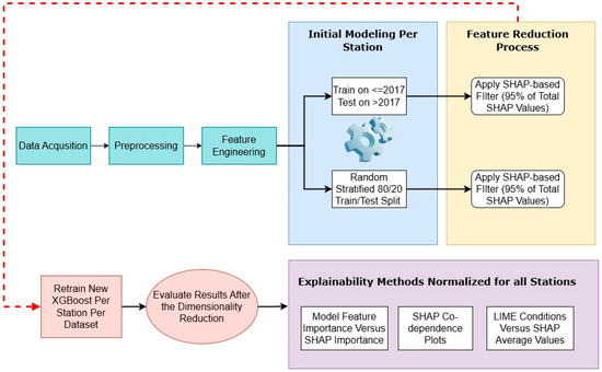
Figure 1.
The complete ML pipeline applied, consisting of data preparation, initial modeling, feature reduction, and explainability.
2.1. Materials
The dataset employed in this study is the Beijing Multi-Site Air-Quality dataset [12], a publicly available resource that contains environmental data collected from 12 monitoring stations across Beijing, China. These stations are equipped with reference-grade instruments that record hourly measurements, providing a detailed and structured dataset suitable for air quality analysis. The dataset spans multiple years, from 1 March 2013 to 28 February 2017, whilst offering a consistent temporal resolution with hourly observations. The recorded air pollutant measurements at each station include PM2.5 (µg/m3), PM10 (µg/m3), SO2 (µg/m3), NO2 (µg/m3), CO (mg/m3), and O3 (µg/m3), capturing a range of airborne contaminants. Each station also collects meteorological data, including air temperature (°C), pressure (hPa), dew point temperature (°C), wind direction (degrees), wind speed (m/s), and precipitation (mm), which describe atmospheric conditions. Additionally, the dataset includes structured temporal information in the form of year, month, day, and hour, ensuring that each data point is accurately time-stamped.
The combination of pollutant concentrations, meteorological variables, and detailed temporal information provides a comprehensive representation of air quality conditions across Beijing. This structured dataset was used in this study to support nowcasting tasks, where PM2.5 concentrations were estimated for each hour using all available environmental and meteorological features except PM2.5 itself.
2.2. Methods
The analysis explores the impact of SHAP-based feature selection on PM2.5 prediction models. Initially, an XGBoost Regressor was trained using all available features from the air quality dataset. Prior to training the model, missing values were imputed using the k-nearest neighbors (KNN) algorithm, with 5 neighbors. This imputation method made the data complete, allowing the features to have consistent values. SHAP values were calculated to assess features’ importance, which formed a new refined feature set. The new refined set of features (applied to train the model) comprised features that made up a total of 95% of the SHAP values.
Following the feature selection process, the models were retrained using the dimensionality reduced feature sets, and their performance was compared to the original model trained with all features. Evaluation metrics such as RMSE and R2 were calculated to quantify performance changes. This comparison was made to highlight the extent of how much the exclusion of low-importance features influenced predictive accuracy, offering insights into the trade-off between model complexity and performance, therefore making the model more explainable and robust.
To assess the effectiveness of the proposed feature selection technique, two evaluation strategies were used. In the first approach, all data prior to 2017 were used for model training, while a three-month time span from 2017 (Jan–March, which was only available) was used as the test set. This method ensured a temporally consistent evaluation, where PM2.5 levels were predicted for each hour using all available features. In the second approach, an 80–20 training–test split was conducted randomly, with the additional condition that each month was represented in the test set. This condition emerged from the need to capture seasonal variability, which is inherently in the air quality data, ensuring the test set reflected a balanced temporal distribution and avoiding biases of specific months that lead to similar patterns. Both evaluation strategies were assessed using RMSE and R2 to ensure consistency with the previous performance analysis. The analysis was conducted for each different station of our dataset both individually and collectively (by aggregating the errors and calculating R2 in the total of 12 stations).
2.2.1. Machine Learning Methods
In our methods, we employed the XGBoost algorithm [13] to model PM2.5 as a nowcasting task. XGBoost (Extreme Gradient Boosting) is a tree-based machine learning algorithm that implements gradient boosting to produce highly accurate predictions. It constructs trees using a histogram-based method, which groups continuous feature values into discrete bins to efficiently identify optimal split points. The general principle is that each new tree is trained to correct the residual errors made by the previous ensemble of trees, typically by splitting on feature thresholds. The model predicts the target variable using the following formulation:
where is the predicted PM2.5 value for input , and is -th tree in the model. The initial prediction starts from a base score (mean value), which is then adjusted by the series of trees. The objective function that is optimized during training includes both a loss term and a regularization term to prevent overfitting:
where represents the error loss between the true value and the observed value . The term is a regularization parameter that controls the tree complexity. Here, is the number of leaves in the tree, is the score assigned to leaf , and is a parameter that penalizes the addition of new leaves to control overfitting. Lastly, is the L2 regularization parameter that reduces large leaf values to avoid overfitting cases.
XGBoost performs a form of internal feature selection by prioritizing features that improve the model’s objective during the tree-splitting process. Features with little predictive power are rarely chosen for splits, resulting in low importance scores. However, this is not a strict feature elimination process; unimportant features remain in the dataset but have minimal influence on the final model. In cases where features are highly correlated, the model may favor one feature while ignoring the other, even if both hold predictive value. XGBoost feature-importance metrics, such as gain or cover, can indicate which features contribute least to the model’s performance. In theory, removing these low-importance features can simplify the model with minimal impact on accuracy, though it is advisable to validate their effect by iteratively assessing performance metrics.
2.2.2. Explainability Methods
The two main explainability-related algorithms that we used were SHAP and LIME. Both algorithms work on a different level and address different problems of explainability; therefore, their usage should be utilized in combination to improve robustness. Firstly, LIME operates on individual points; it explains a single estimation by creating a local approximation of the model around that specific instance (data point). It alters the input by a slight amount (adding some noise) and observes the error generated by this alteration whilst building a simpler, more interpretable model (i.e., a linear regression model). The main principle is to illustrate the original model by using a simple version for a specific prediction. Therefore, it explains why the model made a specific estimation for this data point. From the mathematical point of view, the aim of LIME is to approximate a (generally complex) model (commonly a classifier, considered a black-box model), near a specific instance using a local surrogate model , representing a family of interpretable models (usually a linear regression model or a simple decision tree). On this basis, LIME tackles the following optimization problem:
where
- f: the original model;
- g: the interpretable surrogate model (i.e., linear regressor);
- πx(z): a proximity measure between the instance x and perturbed sample z ( where Z is the set of samples generated around instance x);
- : a local fidelity loss function that ensures the surrogate model g closely approximates model f in the neighborhood of instance x;
- : a complexity penalty for the model g, promoting interpretability (e.g., sparsity in a linear model).
On the other hand, SHAP operates on a global level by considering all predictions in total. It considers the model itself (that works as input) with the final predictions to estimate the so-called Shapley values for each feature that was used to produce those predictions. SHAP is a model-agnostic interpretability method that bases its function in cooperative game theory, more specifically from Shapley values. Shapley values were originally introduced to fairly distribute a total reward among players in a cooperative game, based on their individual contribution [14]. In our case, each training feature represents a “player” and the model output is the total “payout”.
The fundamental idea behind SHAP is that each feature importance is estimated by its contribution to every possible subset of features. Given a set of features and a model function , the Shapley value for a specific feature is given by
where is a subset of features excluding , represents the model’s output when only features in are present, and is the total number of features. The fraction within the sum represents a weighting factor, as it calculates the distribution of all possible sequences of features where the subset appears right before adding the feature . Therefore, this fraction serves the purpose of weighting the term and ensures that each contributor (player, i.e., feature) is fairly averaged without giving more importance to specific features by chance.
2.3. Preprocessing
To prepare the data for modeling, several preprocessing steps were applied. Wind direction was originally recorded as a categorical variable with multiple possible values (NNW, N, NW, NNE, ENE, E, NE, W, SSW, WSW, SE, WNW, SSE, ESE, S, SW). Since most machine learning models work with numerical inputs, we transformed this variable into multiple binary indicators using one-hot encoding. This approach enables the model to distinguish between different wind directions without introducing a false sense of order between categories [15].
The dataset contained missing values in various columns, which could impact model training and performance in an uncertain way. To address this, we used a k-nearest neighbors imputation method. This technique estimates missing values based on the values of the closest data points (neighbors), allowing us to preserve valuable information without discarding rows or columns unnecessarily. We chose this method because it considers relationships between variables and generally provides more accurate imputations compared to simpler approaches like filling with the mean.
2.4. Feature Engineering and SHAP-Based Feature Reduction
To enhance model performance while preserving interpretability, we applied automated feature engineering using lagged variables and evaluated their effect dynamically. Lagged features were created for basic environmental variables—PM10, TEMP, PRES, DEWP, and WSPM—at multiple time intervals (1, 2, 3, 6, 9, 12, 15, 18, 24, 36, and 48 h). These lags capture temporal dependencies and correlations that are often relevant in air quality dynamics as well as in time-series analyses. We also ensured that this process did not negatively impact our modeling performance as we compared the model’s R2 and RMSE values before and after the generation of lagged variables and showed a positive impact on the model’s metrics.
After this step, SHAP-based feature reduction was applied. SHAP values were computed using the training data, and only the subset of features accounting for 95% of the total SHAP importance was retained. The model was then retrained on this dimensionality-reduced feature set. This entire procedure was applied independently for each monitoring station, allowing the model to adapt feature selection to the specific environmental context of each location. We evaluated performance before and after SHAP-based feature reduction using RMSE and R2 scores for each station but also collectively as an average of all stations.
3. Results
3.1. Feature-Related Performance
To evaluate the effectiveness of SHAP-based feature reduction, we conducted experiments under three different settings: a temporal split using data before 2017 for training and 2017 for testing, a randomly stratified (each month to be represented in the dataset) 80/20 split, and a third setup that incorporated lagged features using the same 80/20 split strategy for all stations. The lagged setup significantly increased the number of input features due to the inclusion of temporal dependencies. Lastly, for the lagged features, we used the same 80/20 split strategy as before the introduction of those features.
As Table 1 indicates, in both the temporal and random splits with or without engineered features, SHAP-based dimensionality reduction led to a modest decrease in feature count (from 27 to 22.7 on average) with negligible impact on model performance (less than 1% reduction of R2). In the lagged scenario, despite the increased dimensionality (from 27 to 84 features on average), SHAP effectively reduced the feature set by approx. 24% while keeping the overall predictive power of the model intact.

Table 1.
Overall evaluation metrics and selected features of dimensionality reduction.
3.2. Station-Level Results with Feature Engineering and SHAP
To better understand the station-specific effects of SHAP-based feature reduction after applying lag-based feature engineering, we report the R2 values before and after the dimensionality reduction for each monitoring station, along with the number of features removed. The lag-related features numbered 55, as there were 11 lags for a chosen set of 5 features (PM10, TEMP, PRES, DEWP, and WSPM). Despite the expanded feature space due to lagged variables, SHAP was able to consistently reduce the number of input features while maintaining or slightly improving performance in most stations in terms of R2 and managing to reduce the RMSE (root mean square error) in the majority of stations (Table 2).
Table 2.
Station-wise results for dimensionality reduction with respect to R2, feature elimination, and RMSE.
Overall, the SHAP-based dimensionality reduction technique we applied was quite effective across all locations, with several stations (such as Dingling, Guanyuan, and Wanliu) experiencing a slight improvement in predictive accuracy after simplifying the model. On average, around 22 features were removed per station, indicating that many of the lagged and original features were either redundant or had a minor impact on the model. These findings demonstrate the value of explainability-informed reduction strategies across diverse spatial monitoring contexts. The slight performance improvements observed in stations such as Guanyuan and Dingling highlight how feature simplification can support generalization.
Figure 2 illustrates the SHAP dependence plots across all stations for the three most important features (PM10, CO, and O3) as well as the most prominent interactions among them. These features were selected based on their highest Spearman’s correlation with the ground truth (PM2.5) values, highlighting their strong influence on the model’s behavior. Each subplot displays the relationship between the raw feature value (x-axis) and its corresponding SHAP value (y-axis), which reflects the feature’s contribution to the model’s prediction for each instance. Positive SHAP values indicate that the feature drives the prediction toward higher PM2.5 concentrations, while negative values suggest a lowering effect on the predicted PM2.5 levels. The interaction between the main feature and the secondary (color) feature is determined based on which secondary feature has the highest correlation with the main feature (i.e., PM10 is correlated the most with CO—PM2.5 is excluded as presented in the SHAP values).
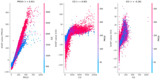
Figure 2.
Co-dependence plots for the top 3 features with the highest correlation (Spearman’s) to SHAP PM10.
This dual encoding allows for the visualization of feature interactions, in line with SHAP’s foundational principle that the effect of one feature may depend on the value of another. For example, in the PM10 case, as PM10 increases, its SHAP value rises almost linearly, indicating a strong and consistent positive contribution to PM2.5 levels (upward—higher PM2.5). The color gradient shows that CO levels further regulate this effect, particularly in the upper range of PM10 values. Similarly, in the CO plot, the relationship between CO concentration levels and SHAP values appears nonlinear and saturates at higher concentrations. This suggests the diminishing contributions of CO to PM2.5 nowcasting beyond a certain level. The PM10 color gradient here enhances the observation that the strength of CO’s impact is conditioned by PM10 concentrations.
Lastly, the O3 plot demonstrates a weaker and more variable relationship with PM2.5 estimations. The slight negative trend suggests that in some contexts, higher ozone levels may correspond to a reduction in nowcasted PM2.5, but the effect is relatively minor compared to PM10 or CO. The variability in the SHAP values across different PM10 interaction levels suggests complex, possibly context-dependent interactions. In summary, this visualization supports the model’s interpretability by highlighting not only which features are most influential but also how their contributions to other predictors change under different conditions.
3.3. XGBoost Model Feature Importance vs. XAI Methods
To investigate the agreement between the model-internal and explainability method’s explanations, we computed the normalized average importance of each feature using both XGBoost’s gain-based importance and SHAP values, aggregated across all stations. The results, presented in Figure 3, illustrate the relative contribution of each feature to the estimation of PM2.5 concentrations.
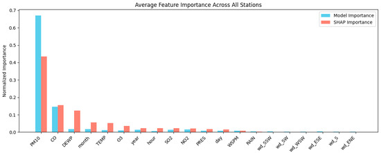
Figure 3.
XGBoost gain-based feature importance vs. SHAP normalized importance averaged for all stations.
Both methods consistently identify PM10 and CO as dominant predictors. However, SHAP reveals a more distributed importance profile, attributing significant weight to features such as TEMP, month, O3, and notably DEWP (dew point). In contrast, the model’s internal importance ranks TEMP, month, O3, and DEWP near zero, suggesting they play an almost negligible role. This discrepancy indicates that SHAP is capturing deeper relationships between an interaction-based effect that the model was unable to adjust even though it had nearly the same performance across all stations (highest reduction in R2 ~1%).
This disparity is especially relevant in cases like DEWP, where the feature may have low standalone importance but nonetheless has inherent influence in interaction with other variables. More generally, SHAP appears to assign moderate importance to a wider range of contextual and meteorological variables, whereas XGBoost’s native importance tends to favor only the strongest predictors that could lead to unnecessary biases in future steps. This comparison highlights the added explanatory depth that SHAP offers in uncovering meaningful but model-suppressed signals.
SHAP provides more detailed explanations, making it especially useful for understanding overall feature importance and how features interact—things that gain-based methods often miss. That said, a potential pitfall of overvaluing raw gain importance is the possibility of making extremely oversimplified interpretations of the dynamics of processes in an environment and potentially undervaluing predictive signals, particularly for predictors—features that have high interaction exhibit low prediction gain (as measured by XGBoost’s main attribution factor) [8], as is the case with dew point. Since air quality dynamics are inherently complex, nonlinear, and operate in multidimensional spaces, XAI methods that allow for feature decomposition are crucial for implementation in practice.
As a next step, both LIME and SHAP results are used to identify features and feature value ranges that contribute to PM2.5 nowcasting.
For this reason, in Figure 4, a comparison of LIME and SHAP values is presented, taking into account different conditions (features and feature value ranges) used in a predictive model, therefore identifying how each feature contributes to the model’s output. The y-axis lists specific conditions or value ranges for our environmental features (e.g., SO2, PM10, CO, and TEMP), while the x-axis shows their corresponding influence values: blue bars represent LIME weights, and red bars represent mean SHAP values across all stations on average. Several key features show strong agreement between LIME and SHAP, both in direction (positive or negative) and approximate magnitude. For example, “TEMP ≤ 3.65”, “TEMP ≤ 3.10”, and “TEMP ≤ 3.00” have consistently high positive values in both LIME and SHAP, indicating that low temperature conditions are strongly associated with increased PM2.5 concentration estimations both locally (individual cases) and globally (on average across the dataset). Similarly, high PM10 levels (e.g., “38.00 < PM10 ≤ 86.00”, “39.00 < PM10 ≤ 91.00”) also show a strong positive influence in both methods, marking them as significant predictors.
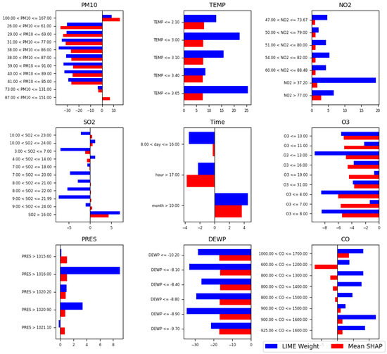
Figure 4.
SHAP averaged values in the top conditions derived from the LIME application for all stations.
Some conditions show moderate agreement but differ in magnitude. For instance, “1000.00 < CO ≤ 1700.00” shows a strong positive SHAP value but a slightly weaker LIME weight, suggesting this condition contributes overall but may have less impact in some local contexts. Conversely, “600.00 < CO ≤ 1200.00” has a strong positive LIME weight but negligible SHAP value, which could mean it has local importance in specific data regions but not when averaged globally.
There are also features where SHAP and LIME diverge notably. For example, “DEWP ≤ −10.20” and nearby dew point ranges show strong negative LIME weights but only small negative SHAP values. This suggests that a very low dew point may strongly influence some individual predictions but is not consistently impactful across the whole dataset.
Coming to O3 (ozone), value ranges such as “O3 ≤ 7.00” and “O3 ≤ 8.00” show modest SHAP contributions but higher LIME values, again highlighting a localized effect. This finding can be attributed to the fact that low O3 levels are usually associated with winter conditions and low photochemical activity, both related to low PM production.
The most significant factors, where both methods strongly agree on their impact, are primarily in the low-temperature and high particulate matter (PM10) ranges. These appear to be key drivers of model estimations across both local and global perspectives. In contrast, disagreement in features such as dew point and certain CO and SO2 ranges shows certain conditions are more important in some instances than throughout the data.
4. Discussion
This study investigated ways in which XAI techniques—SHAP and LIME in this case—can enhance the interpretability of machine learning (ML) models for real-time PM2.5 modeling. While accuracy is still a consideration, especially in an important area such as AQ prediction, this work argues that knowing how the model came to its predictions is just as important. This matter of clarity is even more important when considering environmental contexts where model predictions can inform public policy, health warnings, or long-term interventions.
4.1. Feature Reduction and Model Performance
A valuable contribution of this research was the effective use of SHAP-based feature reduction where we retained features that explained 95% of the total SHAP importance. Importantly, this feature reduction resulted in a negligible decrease in performance, and in some instances, an improvement in performance. This supports the idea that many input features— even those with measurements in the modeled context—may be redundant or contribute very little to the model’s decision making. The findings are in alignment with the existing research that SHAP is a powerful method to explain models, but it can also assist models to reach a more efficient design without sacrificing accuracy [8,11,16] and aligns with the existing literature acknowledging that features of some environments (e.g., urban zones that are impacted by complex microclimates) can benefit from explainability frameworks [4,17].
Across the different evaluation strategies—temporal split, stratified random split, and lag-enhanced training—our models maintained or even improved their R2 scores post-reduction while also showing some significant reduction in RMSE at some stations. Particularly in the lagged-feature scenario, SHAP reduced the input dimensionality by approximately 24% (from 84 to around 67) without sacrificing accuracy. This demonstrates that even in high-dimensional time-series analyses, SHAP can serve as an effective tool for evaluating redundant or noisy features. From a computational standpoint, lighter models are not only faster to train and deploy but are also less prone to overfitting—a concern especially relevant in real-time or near-real-time prediction environments like air quality monitoring [4,18].
4.2. Interpretability
To better understand how individual features influence predictions—and how they interact—we used SHAP dependence plots aggregated across all stations. These plots visualize the relationship between a feature’s raw value and its SHAP value, while using color to represent the value of the most interacting feature. This dual encoding is one of the most compelling strengths of SHAP: it can identify nonlinear interactions between features that traditional feature-importance metrics or even LIME often miss [10]. The three most important features identified via SHAP co-dependence analysis were PM10, CO, and O3. These were selected based on their high Spearman’s or Pearson’s correlation with the model’s output across all stations. In the PM10 subplot, we observed a clear linear trend: as PM10 levels increased, SHAP values also rose, indicating that higher PM10 levels consistently contributed to higher PM2.5 predictions. This is expected as PM2.5 is a fraction of PM10, and therefore they are strongly correlated. The color gradient, reflecting CO values, revealed an important interaction effect—CO appeared to amplify the PM10 contribution, especially at higher pollution levels. This means that with increasing PM concentrations, CO becomes the prominent predictor of PM2.5 rise, giving insight into the PM main emission sources (the same that contribute to CO high levels) in Beijing during the examined period. This kind of conditional influence would be difficult to uncover using traditional univariate analysis. The CO subplot (Figure 2) showed a different pattern: its relationship with SHAP values was nonlinear and saturated at higher concentrations. This saturation indicates that while CO plays a significant role in modeling PM2.5, its marginal contribution diminishes beyond a certain point—a pattern often seen in environmental phenomena dominated by threshold-related approaches [19]. Interestingly, the CO plot’s color gradient again featured PM10 as the interacting variable, further reinforcing the importance of this relationship. This result may suggest that CO-related emission sources (i.e., engine combustions) play an important role in growing PM2.5 concentrations, nevertheless when these concentrations are elevated, then the incremental impact of CO on PM2.5 diminishes. This suggests additional emission sources (like household heating or long-range transport) as the main parameters shaping high PM2.5 values. Such two-sided interactions (PM10 affecting CO’s impact and vice versa) emphasize the need for methods like SHAP that can account for feature synergy rather than treating predictors independently.
The O3 subplot exhibited a weaker and more variable trend. There was a modest negative relationship between ozone levels and SHAP values, suggesting that in some contexts, higher ozone levels may slightly reduce PM2.5 predictions, probably suggesting the suppression of household heating as an emission mechanism during the warmer period of the year. However, the color encoding again pointed to PM10 as a key modulating factor. These more nuanced effects highlight the model’s capacity to detect context-dependent behaviors and demonstrate how SHAP can uncover relationships that may be both subtle and dynamic in real-world environmental systems [5,11].
Another contribution of this study is the comparison between SHAP values and XGBoost’s internal gain-based feature importance. The results show substantial agreement in the top predictors—PM10 and CO appear at the top of both rankings—but diverge significantly in mid- and lower-ranked features. SHAP assigned moderate importance to variables like dew point (DEWP) and month (relevant to seasons of the year), which were almost entirely ignored by XGBoost’s gain scores. This is not surprising because tree-based models such as XGBoost often focus on individual features that have strong effects to start off in model construction [16,18]. When features are important only through some interaction, they may be overlooked altogether in special cases of feature contribution. This framing of model-internal metrics can be particularly limiting in high-dimensional domains such as environmental studies, where environmental variables often co-vary. The dew point might not be a particularly good predictor by itself, but it changes the effects associated with temperature or given PM concentrations by having a role through its influence on humidity levels. SHAP is able to recognize dew point’s contribution because it is averaging feature contributions across many random permutations of contributions, meaning that dependent, interaction effects are largely preserved through modeling [14,20].
Where SHAP is giving a global picture of importance, LIME provides greater local interpretability, which explains individual predictions. When both SHAP and LIME agree on the importance of a feature, this can really help solidify the interpretation. In our results, temperature and PM10 were consistently identified as contributory by both SHAP and LIME, affirming their status as the main drivers of PM2.5 in Beijing, consistent with previous research that has shown temperature inversions and particulates are often correlated in polluted urban environments [1,6]. Nevertheless, we also found several examples of divergence between SHAP and LIME. Distinct ranges of CO and O3 concentration identified as very locally important (LIME) had no global SHAP. Conversely, dew point was identified as an important SHAP feature due to interaction effects but tended to not be narrowly identified as important by LIME. In this case, the differences are not wrong but instead illustrate different interpretability goals. LIME is good at finding specific local behaviors, whereas SHAP demonstrates model structure and synergies across behaviors. These two complementary utility tools can be essentially useful in different contexts [9,21].
4.3. Application Considerations
From the application point of view, considering how to consolidate the size of the model, if possible, to improve human usability seems important. If, for example, it can be shown that a smaller set of predictor variables has almost identical predictive power, then sensor networks can be designed to measure/monitor accordingly. In resource-constrained settings, it may be worth deprioritizing for the least important variables, reducing operational costs while still ensuring reasonable coverage/monitoring and strong predictive capability. This might be quite useful in developing countries in which dense sensor networks are less feasible [1,2]. Furthermore, if models are interpretable, they are more likely to be trusted by policy makers and stakeholders. Ideally, their “black-box” counterparts can explain how they make predictions in coherent, evidence-based ways; in many public health considerations, such as issuing pollution warnings or depending on an output to adjust urban transport initiatives, this is particularly useful [22,23].
4.4. Limitations
Despite the promising results, this study has several limitations. First, it focuses exclusively on XGBoost, an ensemble tree-based algorithm. While this model is widely used and respected for its performance, future research should explore how well the findings generalize to other model families, such as deep neural networks or hybrid ensemble methods, i.e., autoencoding models or multilayer perception models [24]. Neural networks, for example, may require different interpretability strategies, and the behavior of SHAP and LIME may differ in those contexts [7,17].
Secondly, the study is geographically restricted to Beijing, which has a distinct pollution profile shaped by its climate, topography, and regulatory landscape. Applying these models and interpretability strategies to other cities—especially those in coastal or mountainous regions—might yield different patterns. Air quality systems are heavily shaped by local conditions, and interaction effects observed in one environment may not hold in another [19]. Expanding the study to other geographies is a necessary next step for ensuring robustness and transferability. While the use of SHAP co-dependence plots allowed us to visualize complex feature interactions, the analysis could benefit from including higher-order interactions, potentially using more advanced techniques like SHAP interaction values or counterfactual explanations [24]. These methods could help uncover multiway dependencies that are not visible in pairwise comparisons alone.
Finally, while SHAP and LIME provide useful explanations, they are still post hoc methods and can be vulnerable to adversarial manipulation or instability [25,26]. Developing models that are interpretable by design—not just via post hoc analysis—remains a long-term goal for the field. Our findings complement and extend previous work in explainable environmental modeling. For example, ref. [27] demonstrated that ensemble models often perform well for air quality prediction but highlighted the difficulty of interpreting them without specialized tools. By contrast, our use of SHAP in a tree-based model provides a balance between performance and interpretability, without requiring more computationally expensive ensemble approaches. More recent studies have also explored XAI in environmental contexts using attention-based deep learning models [28] or graph-based models for spatiotemporal dependencies [5], but these approaches can be opaque and computationally intensive. Our study suggests that interpretable models like XGBoost, enhanced with SHAP explanations, offer a scalable and accurate alternative for modeling tasks—especially when deployed across multiple stations with varying data completeness.
Furthermore, unlike conventional methods or black-box optimization techniques [24], SHAP operates natively within the model’s architecture and data structure, requiring no custom loss functions or sampling strategies. This makes it more suitable for real-world applications, where model transparency and ease of deployment are key considerations. In terms of real-world application, our findings have direct relevance to both environmental agencies and public health stakeholders. As cities increasingly rely on data-driven systems to guide air quality management, the ability to explain not only what the model predicts but also why is essential for building trust. For instance, if a model signals an upcoming PM2.5 spike, city planners can refer to SHAP outputs to identify which other pollutant precursors (e.g., CO) are driving the change. This in turn enables more targeted and informed interventions, such as traffic control, industrial regulation, or public alerts [1,2].
Equally important is the potential for these models to support long-term environmental planning. Understanding how variables like seasonality, wind direction, or urban heating contribute to pollution can guide infrastructure investments and zoning decisions. A model that merely “predicts well” but offers no interpretability cannot fulfill this broader planning role [7,28].
Moreover, explainability plays a central role in environmental justice. In many cities, pollution exposure is not evenly distributed. Models that explicitly show which features matter—and how those features interact—can help identify whether some areas are consistently underserved by current mitigation strategies. By pairing SHAP explanations with demographic data, future work could assess whether vulnerable populations are disproportionately affected and whether the model’s predictions (and errors) vary by region, class, or ethnicity [23,29]. This study also emphasizes reproducibility—a core value in both machine learning and environmental science. By using open frameworks (SHAP, LIME, XGBoost), common evaluation strategies, and clear hyperparameter settings, we aim to make the findings not only interpretable but also verifiable. Reproducibility is particularly crucial in multisource, multistation problems, where differences in data collection or preprocessing can dramatically affect model outputs.
4.5. Future Prospects
Our aggregation approach (averaging SHAP values across stations and aligning on common features) provides a template for future work across distributed sensor networks. Rather than building a separate model for each site or naively merging heterogeneous data, our method offers a principled way to compare and consolidate model behavior across contexts. This type of methodological clarity enhances both trust and scalability. One promising direction for future research is the integration of counterfactual explanations. These methods, which identify the smallest change needed to flip a model’s prediction, can help stakeholders understand thresholds and risk boundaries [24]. For instance, if a region is about to cross a pollution threshold, counterfactuals could indicate which variable(s) must change—and by how much—to remain below the limit. This offers a more actionable interpretation than SHAP alone and aligns closely with regulatory use cases.
In addition, exploring temporal explainability—how the importance of features evolves over time—could deepen our understanding of seasonality and event-based pollution spikes. While our current model uses temporal splits for validation, the SHAP values themselves are static with respect to time. Using time-series SHAP or other longitudinal techniques could uncover recurring patterns and long-term shifts in pollution dynamics.
Another area for exploration is multimodal data fusion, including possibly satellite imagery, meteorological forecasts, and/or social media signals (X formerly Twitter) [30]. While our current model relies on structured environmental measurement data, many researchers have shown that multimodal models can improve both accuracy and generalizability. Ensuring that these richer models remain interpretable will be a major challenge for the field, but one that is essential if XAI is to remain aligned with its real-world goals [8,21]. Finally, model governance remains an open issue. Even interpretable models can be misused or misunderstood. Developing human-in-the-loop systems, where domain experts can query, validate, and contest model outputs, would greatly increase trust and robustness, and in this state, XAI applications could be considered mandatory.
5. Conclusions
This research assessed the use of SHAP (SHapley Additive exPlanations) and LIME (Local Interpretable Model-agnostic Explanations) as explainability methods of an XGBoost model, for the task of PM2.5 nowcasting. One important issue to note is that accuracy and interpretability are not antithetical to one another. Although SHAP feature reduction resulted in a meaningful reduction in model size, the predictive outcomes were still strong (R2 > 0.93 across all validation configurations). This was most significant by considering lagged variables and still produced a compression in the model in terms of SHAP importance.
While SHAP produced a summary of the relative importance and interactions of the features, LIME summaries provided instance-level explanations. SHAP and LIME help users of information on public health and environmental policy find trust and transparency in them as well. They produced complementary ways of understanding the model’s behavior and utility using both broad and specific scopes. There is still the potential to provide recommendations purely from some metrics of model performance, which may be ignored if tuned to be narrowly model performance driven. These approaches to model evaluation are particularly relevant in developing settings where sensor networks are sparse, and so these lightweight models, although interpretable, can also be implemented operationally for near-real-time application if data is constraining their usefulness.
Because we focused only on one tree-based model, we recommend future research to evaluate the breadth of how applicable these methods are, through all model architectures, geographies, and modalities. We recognize counterfactual explanations and fairness as some exciting research directions. In brief, as we move toward creating models that can be interpretable but also high performing statistically, it will be necessary to use AI responsibly and build trust for environmental decision making.
Author Contributions
Conceptualization, T.T. and K.K.; methodology, T.T. and K.K.; software, T.T.; validation, T.T. and K.K.; formal analysis, T.T. and K.K.; investigation, T.T.; resources, T.T., T.K., E.B. and K.K.; data curation, T.T., T.K. and E.B.; writing—original draft preparation, T.T.; writing—review and editing, T.T., T.K., E.B. and K.K.; visualization, T.T.; supervision, K.K.; project administration, K.K.; All authors have read and agreed to the published version of the manuscript.
Funding
This research received no external funding.
Institutional Review Board Statement
Not applicable.
Informed Consent Statement
Not applicable.
Data Availability Statement
Data are available in via Zhang et al., 2017 [12].
Conflicts of Interest
The authors declare no conflicts of interest.
References
- World Health Organisation. WHO global air quality guidelines: Particulate matter (PM2.5 and PM10), ozone, nitrogen dioxide, sulfur dioxide and carbon monoxide. In World Health Organisation Guidelines; World Health Organisation: Geneva, Switzerland, 2021. [Google Scholar]
- Wu, J.; Chen, X.; Li, R.; Wang, A.; Huang, S.; Li, Q.; Qi, H.; Liu, M.; Cheng, H.; Wang, Z. A novel framework for high resolution air quality index prediction with interpretable artificial intelligence and uncertainties estimation. J. Environ. Manag. 2024, 357, 120785. [Google Scholar] [CrossRef] [PubMed]
- Li, X.; Peng, L.; Hu, Y.; Shao, J.; Chi, T. Deep learning architecture for air quality predictions. Environ. Sci. Pollut. Res. Int. 2016, 22, 22408–22417. [Google Scholar] [CrossRef] [PubMed]
- Salman, A.K.; Choi, Y.; Singh, D.; Kayastha, S.G.; Dimri, R.; Park, J. Temporal CNN-based 72-h ozone forecasting in South Korea: Explainability and uncertainty quantification. Atmos. Environ. 2025, 343, 120987. [Google Scholar] [CrossRef]
- He, Z.; Guo, Q. Comparative Analysis of Multiple Deep Learning Models for Forecasting Monthly Ambient PM2.5 Concentrations: A Case Study in Dezhou City, China. Atmosphere 2024, 15, 1432. [Google Scholar] [CrossRef]
- Li, L.; Zhang, R.; Sun, J.; He, Q.; Kong, L.; Liu, X. Monitoring and prediction of dust concentration in an open-pit mine using a deep-learning algorithm. J. Environ. Health Sci. Eng. 2021, 1, 401–414. [Google Scholar] [CrossRef] [PubMed]
- Doshi-Velez, F.; Kim, B. Towards a Rigorous Science of Interpretable Machine Learning. arXiv 2017, arXiv:1702.08608. [Google Scholar]
- Molnar, C. Interpretable Machine Learning; Lulu.com: Morrisville, NC, USA, 2020. [Google Scholar]
- Ribeiro, M.T.; Singh, S.; Guestrin, C. “Why Should I Trust You?”: Explaining the Predictions of Any Classifier. In Proceedings of the 22nd ACM SIGKDD International Conference on Knowledge Discovery and Data Mining, San Francisco, CA, USA, 13–17 August 2016; pp. 1135–1144. [Google Scholar]
- Lundberg, S.M.; Lee, S.I. A Unified Approach to Interpreting Model Predictions. Adv. Neural Inf. Process. Syst. 2017, 30, 4768–4777. [Google Scholar]
- Tasioulis, T.; Karatzas, K. Reviewing Explainable Artificial Intelligence towards Better Air Quality Modelling. In Advances and New Trends in Environmental Informatics 2023; Wohlgemuth, V., Kranzlmüller, D., Höb, M., Eds.; Progress in IS; Springer: Cham, Switzerland, 2024; pp. 3–20. ISBN 978-3-031-46901-5. [Google Scholar]
- Zhang, S.; Wu, S.; Liu, Y.; He, K. Cautionary Tales on Air-Quality Improvement in Beijing. Proc. R. Soc. A Math. Phys. Eng. Sci. 2017, 473, 20170457. [Google Scholar] [CrossRef] [PubMed]
- Chen, T.; Guestrin, C. XGBoost: A Scalable Tree Boosting System. In Proceedings of the 22nd ACM SIGKDD International Conference on Knowledge Discovery and Data Mining, San Francisco, CA, USA, 13–17 August 2016; pp. 785–794. [Google Scholar]
- Shapley, L.S. A Value for n-Person Games. In Contributions to the Theory of Games; Kuhn, H.W., Tucker, A.W., Eds.; Princeton University Press: Princeton, NJ, USA, 1953; Volume II, pp. 307–317. [Google Scholar]
- Poslavskaya, E.; Korolev, A. Encoding Categorical Data: Is There Yet Anything ‘Hotter’ Than One-Hot Encoding? arXiv 2023, arXiv:2312.16930. [Google Scholar]
- Lundberg, S.M.; Erion, G.G.; Chen, H.; DeGrave, A.; Prutkin, J.M.; Nair, B.; Katz, R.; Himmelfarb, J.; Bansal, N.; Lee, S.I. From Local Explanations to Global Understanding with Explainable AI for Trees. Nat. Mach. Intell. 2020, 2, 56–67. [Google Scholar] [CrossRef] [PubMed]
- Meng, C.; Huang, K.; Wu, Y.; Wang, Y.; Liu, M.; Zhang, M.; Li, Z. Interpretability and Fairness Evaluation of Deep Learning Models on MIMIC-IV Dataset. Sci. Rep. 2022, 12, 7166. [Google Scholar] [CrossRef] [PubMed]
- Strumbelj, E.; Kononenko, I. Explaining Prediction Models and Individual Predictions with Feature Contributions. Knowl. Inf. Syst. 2014, 41, 647–665. [Google Scholar] [CrossRef]
- Seinfeld, J.H.; Pandis, S.N. Atmospheric Chemistry and Physics: From Air Pollution to Climate Change, 3rd ed.; John Wiley & Sons: Hoboken, NJ, USA, 2016. [Google Scholar]
- Gilpin, L.H.; Bau, D.; Yuan, B.Z.; Bajwa, A.; Specter, M.; Kagal, L. Explaining Explanations: An Overview of Interpretability of Machine Learning. In Proceedings of the 2018 IEEE 5th International Conference on Data Science and Advanced Analytics (DSAA), Turin, Italy, 1–3 October 2018; pp. 80–89. [Google Scholar]
- Arya, V.; Bellamy, R.K.E.; Chen, P.Y.; Dhurandhar, A.; Hind, M.; Hoffman, S.C.; Houde, S.; Liao, Q.V.; Luss, R.; Mojsilović, A.; et al. One Explanation Does Not Fit All: A Toolkit and Taxonomy of AI Explainability Techniques. arXiv 2019, arXiv:1909.03012. [Google Scholar]
- Gunning, D.; Aha, D. DARPA’s Explainable Artificial Intelligence (XAI) Program. AI Mag. 2019, 40, 44–58. [Google Scholar]
- Binns, R. Fairness in Machine Learning: Lessons from Political Philosophy. In Proceedings of the Conference on Fairness, Accountability and Transparency (FAT), PMLR, New York, NY, USA, 23–24 February 2018; pp. 149–159. [Google Scholar]
- Verma, S.; Dickerson, J.P.; Hines, K. Counterfactual Explanations and Algorithmic Recourses for Machine Learning: A Review. ACM Comput. Surv. 2024, 56, 312. [Google Scholar] [CrossRef]
- Slack, D.; Hilgard, S.; Jia, E.; Singh, S.; Lakkaraju, H. Fooling LIME and SHAP: Adversarial Attacks on Post Hoc Explanation Methods. In Proceedings of the AAAI/ACM Conference on AI, Ethics, and Society, New York, NY, USA, 7–8 February 2020; pp. 180–186. [Google Scholar]
- Alvarez-Melis, D.; Jaakkola, T.S. On the Robustness of Interpretability Methods. arXiv 2018, arXiv:1806.08049. [Google Scholar]
- Campanile, L.; Cocchia, E.; Nappi, M.; Ricciardi, S.; Sessa, S. Ensemble Models for Predicting CO Concentrations: Application and Explainability in Environmental Monitoring in Campania, Italy. Proc. Eur. Counc. Model. Simul. 2024, 38, 558–564. [Google Scholar]
- Jimenez-Navarro, M.J.; Camara, A.; Martinez-Alvarez, F.; Troncoso, A. Explainable Deep Learning on Multi-Target Time Series Forecasting: An Air Pollution Use Case. Results Eng. 2024, 24, 103290. [Google Scholar] [CrossRef]
- Mehrabi, N.; Morstatter, F.; Saxena, N.; Lerman, K.; Galstyan, A. A Survey on Bias and Fairness in Machine Learning. ACM Comput. Surv. (CSUR) 2021, 54, 115. [Google Scholar] [CrossRef]
- Liu, X.; Peng, B.; Wu, M.; Wang, M. Occupation Prediction with Multimodal Learning from Tweet Messages and Google Street View Images. Agil. GIScience Ser. 2024, 5, 36. [Google Scholar] [CrossRef]
Disclaimer/Publisher’s Note: The statements, opinions and data contained in all publications are solely those of the individual author(s) and contributor(s) and not of MDPI and/or the editor(s). MDPI and/or the editor(s) disclaim responsibility for any injury to people or property resulting from any ideas, methods, instructions or products referred to in the content. |
© 2025 by the authors. Licensee MDPI, Basel, Switzerland. This article is an open access article distributed under the terms and conditions of the Creative Commons Attribution (CC BY) license (https://creativecommons.org/licenses/by/4.0/).