Modeling the Risks of Poisoning and Suffocation in Pre-Treatment Pools Workshop Based on Risk Quantification and Simulation

Abstract

Poisoning and suffocation accidents occurred frequently in the pre-treatment pool workshops of biogas plants, so this paper provided a multi-dimensional risk analysis model: Bow-Tie-Qualitative Comparative Analysis (QCA)-Bayesian Neural Network-Consequence Simulation. First, the reasons for biogas poisoning and suffocation accidents were clarified through Bow-Tie. Then, the QCA method explored the accident cause combination paths in management. Next, the frequency distribution of biogas poisoning and suffocation accidents in the pre-treatment pool workshop was predicted to be 0.61–0.66 using the Bayesian neural network model, and the uncertainty of the forecast outcome was given. Finally, the ANSYS Fluent 16.0 simulation of biogas diffusion in three different ventilation types and a grid-independent solution of the simulation were conducted. The simulation results showed the distribution of methane, carbon dioxide and hydrogen sulfide gases and the hazards of the three gases to workers were analyzed. In addition, according to the results, this paper discussed the importance and necessity of ventilation in pre-treatment pool workshops and specified the hazard factors in biogas poisoning and suffocation accidents in the pre-treatment pool workshops. Some suggestions on gas alarms were also proposed.

1. Introduction

As energy demand continues to grow, the development of alternative energy sources has become increasingly urgent [1,2,3,4]. Vigorously developing biogas plants is one of the important measures to achieve energy diversification and sustainable development goals [5,6,7,8]. This process not only reduces the emission of potent greenhouse gases (methane), but also promotes the development of a circular economy [9,10,11]. China has introduced a series of policies to encourage provinces to build large and medium-sized biogas plants in accordance with local conditions and to promote standardized scale breeding and comprehensive utilization of livestock and poultry waste [12,13]. However, the development of biogas engineering technology still faces some challenges. This paper counted a total of 179 biogas accidents that occurred from 2009 to 2024, including 121 biogas poisoning and suffocation accidents, which caused a total of 396 deaths and 134 injuries. Biogas accidents often occur in pre-treatment pool workshops. Statistical data show that in the past 16 years, the number of poisoning and suffocation accidents in the development of biogas plants accounted for as high as 67.6% of the total number of accidents, and these accidents caused serious casualties. Therefore, conducting risk quantification analysis on poisoning and suffocation accidents in pre-treatment pool workshops and proposing effective control measures are issues that need to be urgently addressed in biogas plants.

Countries around the world are also actively taking measures to ensure the safe operation of biogas plants. The German Biogas Association has developed guidelines for the design, construction and operation of biogas plants, including hazard identification and assessment and safety management systems, and has also established laws to limit the emission concentrations of biogas plants [14]. The United Kingdom, the United States and Canada have also developed standards for risk identification and assessment of biogas plants, which require that biogas plants should set up safety management organizations, provide regular safety training for employees and perform regular maintenance of equipment [15].

In terms of accident causes analysis, Scarponi et al. analyzed the risk factors (such as poisoning and explosion) in each part of biogas projects and conducted a sensitivity analysis [16]. By emphasizing intrinsic safety, it strives to choose a safer solution in the design stage. Risk assessment models such as DyPASI-Dynamic Procedure for Hazard Identification, HAZOP, the consequences-based approach, multi-criteria decision-making and FTOPSIS-HAZOP identified the key hazard factors and causal chains in the entire biogas production process [17,18]. In terms of the frequency and consequence of accidents, previous studies had obtained the frequency of poisoning and suffocation accidents in biogas plants through accident statistics [19,20,21,22,23,24], and these researchers studied the physical and chemical properties of hydrogen sulfide and concluded that the acute toxicity of hydrogen sulfide is the main cause of biogas poisoning and suffocation accidents, and emphasized that poisoning and suffocation accidents should be taken seriously by enterprises. Additionally, some studies have demonstrated through on-site measurements and PHAST v6.7 software numerical simulation that biogas indeed caused personnel poisoning and suffocation [25,26], and have concluded the scope of the hydrogen sulfide poisoning area and safe operating measures after biogas leakage. For risk prediction using AI, the dynamic Bayesian network (DBN) method [27] has been used in probabilistic safety assessment and reliability research by modeling a fault time series. Support vector machines (SVMs) [28], deep neural networks (DNNs) and tunicate swarm algorithms (TSAs) [29] can assess and predict disease risks. Long short-term memory networks (LSTMs) [30], convolutional neural networks (CNNs) and bidirectional long short-term memory (BiLSTM) [31] models can predict traffic accident risks. A multi-model approach [32] integrating Bayesian Networks (BN), Machine Learning (ML) models, Natural Language Processing (NLP) with Sentiment Analysis, Agent-Based Modeling (ABM), and Survival Analysis to predict causal relationships in high-risk steel industry accidents was used. The Management Oversight and Risk Tree (MORT) was combined with machine learning algorithms [33] to derive a risk prediction model for hydrogen leakage accidents. S Senthilraj et al. [34] provided sufficient conditions for stability that are time-delay dependent for GRN systems with specific complex structures, thus, advancing the theory of stability of dynamical systems. The research in this paper is rooted in industrial risk analysis, and its core is to develop and apply a multidisciplinary integrated practical framework to solve specific safety risk quantification problems. However, the high rigor of the study by S Senthilraj et al. can provide inspiration for future work in risk quantification.

However, these studies failed to provide a comprehensive analysis of the causal logic underlying biogas poisoning and suffocation accidents and have not thoroughly investigated the interplay among management factors contributing to such incidents. Additionally, limited research has been conducted on accident probability prediction and consequence simulation. To address these gaps, this paper proposed a multi-dimensional risk analysis framework: “accident causality-management-probability-consequence simulation,” namely, the Bow-Tie-Qualitative Comparative Analysis (QCA)-Bayesian Neural Network-Consequence Simulation model. Compared with traditional methods such as HAZOP [35], FTA [36], and FMEA [37], the Bow-Tie [38] model offers the ability to simultaneously analyze the causal logic and impact of accidents, constructing a complete causal chain. The QCA [39] method excels in exploring the combination paths of causes within accident management through case studies. In contrast to conventional Bayesian models, the Bayesian neural network [40] model leverages deep learning to predict accident probabilities while incorporating Bayesian principles to quantify prediction uncertainties, thereby minimizing subjective influences. Commonly used consequence simulation tools include ANSYS Fluent [41], PHAST [42], and ALOHA [43]. ANSYS Fluent stands out for two reasons: it allows customization of leaked gas components and proportions, and it mandates grid-independent solution verification during simulations, enhancing the reliability of the results.

In this paper, the Bow-Tie-QCA-Bayesian Neural Network-Consequence Simulation model was applied to conduct a quantification analysis on the poisoning and suffocation risk of the pre-treatment pool workshop. First, we clarified the causes of biogas poisoning and suffocation accidents in the pre-treatment pool workshop through Bow-Tie. Then, the QCA method explored the accident cause combination paths in management. Next, the Bayesian neural network model was used to predict the accident frequency distribution. Finally, the diffusion consequences of biogas in the pre-treatment pool workshop were numerically simulated in three different ventilation types using ANSYS Fluent. In addition, according to the results, this paper discussed the importance and necessity of ventilation in pre-treatment pool workshops, and specified the hazard factors in biogas poisoning and suffocation accidents in the pre-treatment pool workshop. Some suggestions on gas alarms were also proposed. This study is expected to provide a basis for the prevention of biogas poisoning and suffocation accidents, and a safe working environment for workers.

2. Methods

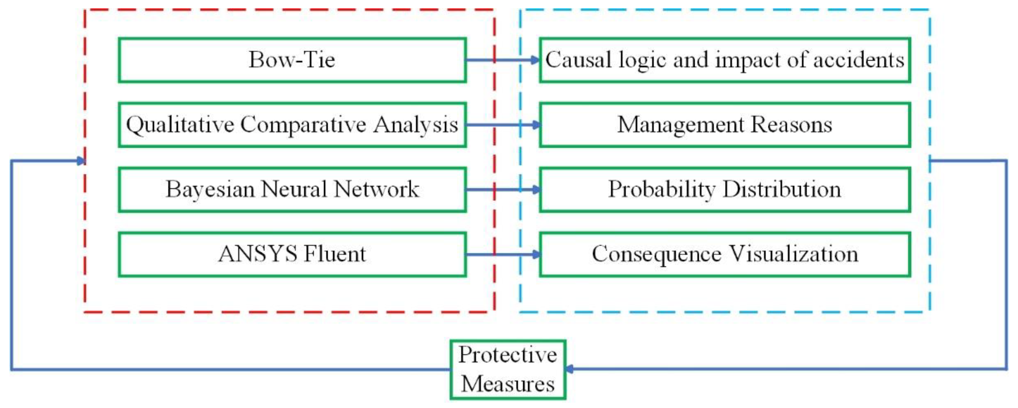
The schematic diagram of the Bow-Tie-QCA-Bayesian Neural Network-Consequence Simulation model is shown in Figure 1. It provides a conceptual overview of the integrated methodological framework employed in this study to comprehensively analyze biogas pre-treatment pool poisoning and suffocation risks. The framework strategically combines four distinct approaches to address different facets of the risk:

Bow-Tie systematically identified the potential causes, critical safety barriers and potential consequences of poisoning and suffocation accidents within the biogas pre-treatment pool environment. It visually mapped out the pathways from initiating events to undesired outcomes. QCA was applied retrospectively to historical accident data. Its role was to uncover complex combinations of management-related conditions that are sufficient for accidents to occur. QCA moved beyond identifying single factors to reveal the configurational causality prevalent in real-world accident scenarios. The primary function of BNN was to quantitatively predict the probability of future accident occurrences based on input variables representing identified risk factors. Crucially, the BNN inherently provides uncertainty estimates associated with its predictions, acknowledging the probabilistic nature of risk. A simulation was employed to evaluate the hazard consequence identified in the Bow-Tie analysis. Control measures were obtained through these methods and then risks were evaluated to form a cycle.

This multi-faceted approach aims to provide a more robust and holistic assessment of biogas poisoning and suffocation risk than any single method alone.

2.1. Bow-Tie

The Bow-Tie model is a widely adopted risk management tool in the domains of safety science and engineering. It derives its name from its distinctive shape, which resembles a bow tie. By integrating the analysis of accident causes with strategies for consequence prevention and control, the model effectively combines ‘pre-event prevention’ and ‘post-event emergency response’, offering an intuitive yet structured framework for managing risks in complex systems [44]. Originating in the petrochemical industry during the 1990s, the Bow-Tie model has since evolved into a cornerstone methodology for risk management in high-risk sectors such as aviation, healthcare and nuclear energy [45].

In the Bow-Tie model, the top event represents the key event that is not expected to occur. The fault tree on the left analyzes the root cause (basic event) of the top event through logical combination (AND/OR gate). The event tree on the right analyzes various consequences that may arise after the occurrence of the top event and the corresponding prevention/mitigation barriers. Bow-Tie has advantages in systematically integrating the causes, consequences and barriers of risks.

2.2. Qualitative Comparative Analysis (QCA)

For the QCA method [46], researchers analyze the relationship between these combinations of conditions and results by constructing truth tables, and use Boolean algebra algorithms to identify the different combinations of conditions that lead to the occurrence of results, namely ‘causal complexity’. In this way, QCA can reveal multiple pathways that lead to the same outcome in different contexts.

At the operational level, the QCA research process includes five stages: case system selection, conditional variable calibration, necessity analysis, derivation of sufficient combination paths, and robustness testing. This method systematically compares case features by constructing a truth table, refines the explanatory model using a Boolean minimization algorithm, and evaluates the explanatory effectiveness of the solution set using coverage and consistency indicators [47].

The steps of QCA include: (1) Identifying research questions and variables; (2) Case selection and data collection; (3) Data calibration; (4) Necessity Analysis; (5) Conditional configuration path analysis; (6) Robustness test. More technical details are presented in Section 3.2.

2.3. Bayesian Neural Networks

Deep learning is mainly based on neural network models, which have been widely used in fields such as reasoning, decision-making and prediction due to their outstanding advantages and powerful capabilities [48]. Currently, deep learning has attracted widespread attention in academia and industry. This study used a Bayesian neural network model to predict the frequency distribution of poisoning and suffocation accidents in the pre-treatment pool of biogas plants. The main reason for choosing the Bayesian neural network model is that the Bayesian neural network model optimizes the mean and variance of the weights. Both the weights and the outputs are probability distributions, which guarantees the reliability and uncertainty of the outputs [49,50]. However, the neural network model optimizes weights, and both weights and outputs are certain values, which makes the model not advantageous in terms of uncertainty and confidence. Markov Chain Monte Carlo or variational inference was used to estimate the posterior distribution [51,52,53]. This article used Python to implement the prediction of the Bayesian neural network.

The inference formula, Gaussian prior and likelihood function of the Bayesian neural network are as follows [54]:

Given a set of data x, we want to predict the corresponding y. A neural network represents this correspondence as a function f(x,θ), where θ is the weight and bias of the neural network. In a Bayesian neural network, weights and biases are probability distributions, so the function f(x,θ) can be expressed as follows:

$$p(y|x,D)={\displaystyle \int P(y|x,\theta )}P(\theta |D)d\theta$$

(1)

where p(y|x,θ) is the likelihood function, which represents the probability of observing the value y given x and θ. p(θ|D) is the posterior distribution of weights and biases given the observed data D.

To make accurate predictions on the data, the following posterior predictive distribution is used:

$$p(y^{\ast }|x^{\ast },D)={\displaystyle \int P(y^{\ast }|x^{\ast },\theta )}P(\theta |D)d\theta$$

(2)

where x* is the new input and y* is the corresponding predicted output.

Our first Bayesian neural network employs a Gaussian prior on the weights and a Gaussian likelihood function for the data.

To train the network, we define a likelihood function comparing the predicted outputs of the network with the actual data points:

$$p(y_i|x_i,\theta )=N(N{N}_{\theta }(x_i,{\sigma }^2),\mathrm{with}\mathrm{prior}\sigma ~\Gamma (1,1)$$

(3)

Here, y_i represents the actual output for the i-th data point, x_i represents the input for that data point, σ is the standard deviation parameter for the normal distribution, and NN_θ is the shallow neural network parameterized by θ.

The model in this article is completed in Python 3.11 software, and the required model is retrieved from the Pyro library.

2.4. ANSYS Fluent Numerical Simulation

ANSYS Fluent 16.0 simulation software performs numerical calculations and image visualization of specific parameters in fluid flow through computers. The basic operating idea of the above software is to perform numerical simulation of fluid under the control of basic flow equations. First, replace the flow field of continuous variables in the spatial domain with a set of variable values at a series of discrete points. Then, an equation or system of equations is established that expresses the relationship between the variables. Finally, we can obtain the distribution of the required variables in the flow field and the distribution of these variables changing with time by solving the equations [55].

In this paper, ANSYS Fluent 16.0 was used to simulate the biogas diffusion of the pre-treatment pool of the biogas plant under different ventilation conditions and to verify the grid-independent solution. Based on the simulation results obtained, the diffusion law of biogas was explored, and corresponding control measures were proposed. The simulation of biogas diffusion in the pre-treatment pool workshop in this study involved the continuity equation, momentum equation, energy equation, species transport model and the standard k-ε turbulence model [56].

The core functional modules of FLUENT include fluid flow simulation, heat transfer and phase change, chemical reaction and combustion, multi-physics field coupling, mesh processing capability, solver technology and data post-processing. It has been widely applied in fields such as aerospace, automotive engineering, energy and power, electronics and electrical appliances, and biomedicine.

The basic assumptions in the simulation process in this paper are as follows:

(1) The diffused gas is treated as an incompressible fluid and presents a turbulent flow state; (2) the diffusion area and biogas diffusion velocity are constant during the biogas diffusion process; (3) the biogas diffusion process does not undergo any chemical reaction or phase change reaction; (4) under the consideration of outdoor wind, it is considered that the air outlet is set perpendicular to the plant, the gas flow direction is perpendicular to the vent, and the wind speed is constant.

3. Results and Discussion

3.1. Causes of Poisoning and Suffocation Accidents in Pre-Treatment Pools

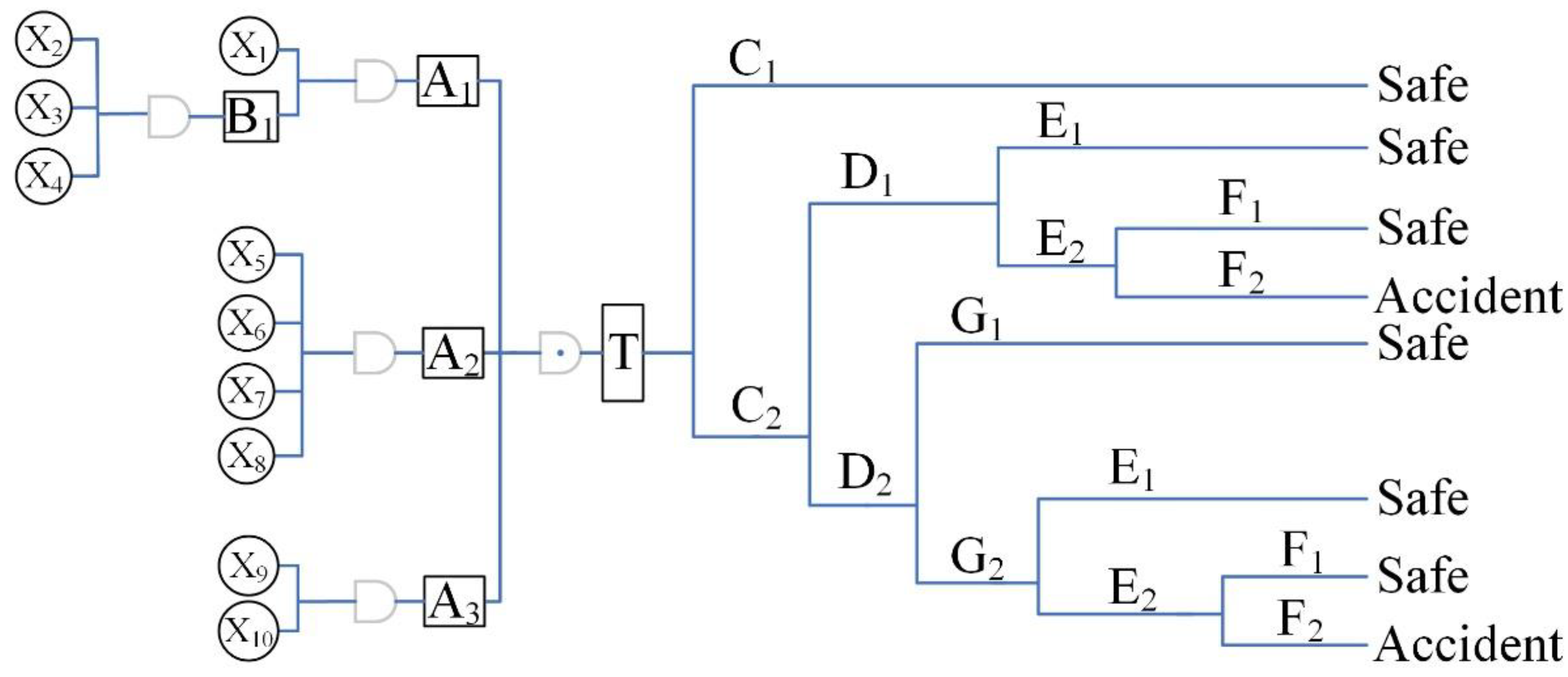
The Bow-Tie model for biogas poisoning and suffocation accidents in pre-treatment pools is presented in Figure 2. The meaning of each symbol can be seen in

Table 1. List of causes of poisoning and suffocation accidents in the pre-treatment pool workshop.

Symbol	Meaning	Symbol	Meaning
T	Biogas poisoning and suffocation in the pre-treatment pool.	X9	Not wearing protective equipment.
A1	Excessive harmful gases.	X10	Failure of the protective equipment.
A2	The workers entered the workshop in violation of regulations.	C1	The harmful gases have not exceeded the standard.
A3	The workers failed to comply with the protective requirements.	C2	Excessive harmful gases.
B1	Failure of forced ventilation system.	D1	No forced ventilation system.
X1	Not setting up forced ventilation.	D2	Installation of forced ventilation system.
X2	Failure of H2S gas detection alarm.	E1	The workers enter the workshop in accordance with the normal regulations.
X3	Failure of interlock between H2S gas detection alarm and forced ventilation system.	E2	The workers entered the workshop in violation of regulations.
X4	Failure of forced ventilation equipment.	F1	The workers carry out the protective requirements.
X5	Failure of gas detection equipment used in environmental testing.	F2	The workers failed to comply with the protective requirements.
X6	Not conducting the environmental testing.	G1	The effective ventilation system.
X7	Excessive gas levels were detected, but forced ventilation was not performed.	G2	Failure of ventilation system.
X8	The gas exceeded the standard and forced ventilation was performed, but it was not diluted to a reasonable concentration.

.

The Bow-Tie model was used to analyze Biogas poisoning and suffocation in the pre-treatment pool. In the Bow-Tie model, the top event represents the biogas poisoning and suffocation accidents in the pre-treatment pool. The fault tree on the left analyzed the root cause of the top event through logical combination, including aspects of the ventilation system, gas detection alarm, protective equipment, and so on. The event tree on the right analyzed consequences after the occurrence of the top event. It can be known from the analysis results that as long as the harmful gases can be controlled within the standard, the top incident will not occur. Effective ventilation equipment, prevention of personnel entering illegally and wearing protective equipment are all effective mitigation barriers.

In accordance with the provisions of ‘Technical Specifications for Biogas Engineering Part 1: Engineering Design’, the pre-treatment pool workshop should be equipped with combustible gas alarm devices and toxic gas alarm devices, namely, a methane gas alarm and a hydrogen sulfide gas alarm. When natural ventilation cannot meet the requirements of the factory, forced exhaust can be used. At this time, the gas alarm devices in the workshop should be interlocked with the forced ventilation facilities.

The pre-treatment pool workshop meets the definition of confined space in the ‘Safety Regulations for Confined Space Operations in Industrial and Trade Enterprises’, that is, confined space refers to a closed or partially closed space not designed as a fixed workplace and can be entered by personnel for work, which is prone to cause hazardous materials accumulation (toxic, harmful, flammable and explosive substances) and insufficient oxygen content. If operators need to enter the pre-treatment pool workshop to carry out operations, the operations are called confined space operations. Before entering the pre-treatment pool workshop, operators must strictly abide by the confined space operation requirements. Before entering, operators must conduct a gas test to check whether the oxygen concentration in the workshop meets the standard. If it does not meet the standard, forced ventilation is required. After the concentration test meets the standard, operators can enter the workshop. In addition, as the pre-treatment pool workshop is prone to biogas poisoning and suffocation accidents, protections such as respiratory equipment and safety belts should be provided.

The Bow-Tie model elucidated the logical relationship for biogas poisoning and asphyxiation accidents. It is evident that the prevention of such incidents can be addressed through the following measures: establishing an efficient forced ventilation system, prohibiting unauthorized entry into the pre-treatment pool workshop by workers, and ensuring strict adherence to protective requirements.

3.2. QCA for Management Reasons: Combination Paths

(1)

Identify research questions and variables

Research question: What combination of management-level factors can lead to poisoning and suffocation accidents in pre-treatment workshop?

Outcome variables: poisoning and suffocation accidents (P) (1 = occurred, 0 = did not occur).

From the analysis results of the bow-tie model in Section 3.1, it can be seen that the causes of poisoning and suffocation accidents in the pre-treatment pool included: no forced ventilation system, forced ventilation failure, accident exhaust failure, no manual switch for accident exhaust, failure of the manual switch for accident exhaust, failure of the harmful gas detection alarm, failure of the interlock between the gas alarm and the ventilation system, operators failing to enter the factory building in accordance with the requirements for confined space operations, and operators failing to implement protection requirements, etc.

From the perspective of management factors, the causes of the above accidents can be summarized into the following variables:

Condition variables: system and procedure management (A), training and education management (B), equipment maintenance management (C), supervision and inspection management (D), safety facility investment (E), emergency and response management (F). (1 = in sufficient, 0 = sufficient)

(2)

Case selection and data collection

Because poisoning and suffocation accidents in pre-treatment tanks cannot meet the sample size requirements, the selection of accidents needed to be expanded to cases of biogas poisoning and suffocation in septic tanks or sewage tanks. Therefore, this article selected a total of 45 biogas poisoning and suffocation accidents from 2021 to 2024, covering industries such as breeding, sewage treatment and environmental protection, thereby reflecting the commonalities and differences of management systems.

(3)

Data calibration. The data of 45 cases of biogas poisoning and suffocation accidents were converted into binary variables (i.e., 0 and 1). The data calibration is shown in

Table 2. QCA calibration table for poisoning and suffocation accidents in pre-treatment pools.

Number	A	B	C	D	E	F	P
1	1	1	1	1	0	1	1
2	1	1	0	1	1	1	1
3	1	1	0	1	0	1	1
4	1	1	0	1	1	1	1
5	1	1	0	1	1	1	1
6	1	1	0	1	1	1	1
7	0	1	1	1	0	1	1
8	1	1	0	1	0	1	1
9	1	1	0	1	0	1	1
10	1	1	0	1	0	1	1
11	1	1	0	1	0	1	1
12	0	1	1	1	0	1	1
13	1	1	0	1	0	1	1
14	1	1	0	1	0	1	1
15	1	1	0	1	0	1	1
…	…	…	…	…	…	…	…
45	1	1	1	1	0	1	1
46	0	1	1	1	0	1	1
47	0	1	1	1	0	1	1
48	1	1	0	1	1	1	1
49	0	1	0	1	1	1	1
50	0	1	0	1	0	1	1

.

(4)

Necessity Analysis. The software fsQCA 4.0 was used to determine whether the six conditional variables were necessary conditions for biogas poisoning and suffocation accidents in the pre-treatment pool. The consistency and coverage of each conditional variable are shown in

Table 3. The consistency and coverage of each conditional variable.

Variable	Consistency	Coverage
A	0.58	1
B	1.00	1
C	0.27	1
D	1.00	1
E	0.33	1
F	0.93	1

.

As can be seen from Table 3, the consistency of conditional variables B, D and F was greater than 0.9, which shows that the above three variables were necessary conditions for the occurrence of biogas poisoning and suffocation accidents. The consistency of variables B and D was one, which indicated that inadequate training and education management and inadequate supervision and inspection management existed in all accident cases. The consistency of the F variable was 0.93, which meant that the reason for inadequate emergency and response management existed in 93% of the accident cases.

Variables A, C and E were not necessary conditions. For system and procedure management (A), even when the system is robust, non-compliance with established procedures by personnel may lead to accidents. For equipment maintenance management (C), despite well-maintained equipment, gas accumulation can still occur in the absence of properly installed ventilation facilities. For safety facility investment (E), even with adequate safety investments, staff members remain at risk of exposure to harmful gases if safety facilities are not utilized as intended.

(5)

Conditional configuration path analysis. In this paper, the consistency threshold was selected as 0.8 and the cutoff value was 1 to perform truth table analysis. The conditional combination path leading to the anaerobic tank explosion accident is shown in

Table 4. Conditional combination paths.

Conditional Combination Paths	Raw Coverage	Unique Coverage	Consistency
Path 1: B * D * F	0.93	0.56	1
Path 2: B *~C * D *~E	0.44	0.07	1
Solution coverage	1
Consistency of solution	1

.

It can be seen from Table 4 that the consistency scores of the above two groups of conditional combination paths were both one, which indicated that these two combination paths had a high degree of explanation for the 45 cases of biogas poisoning and suffocation accidents. Moreover, the consistency score of the solutions was greater than 0.8, and the coverage of the solutions was one, which meant that these two groups of solutions can well explain the path of the accident.

In Path 1, if the three aspects of training and education management, supervision and inspection management, and emergency and response management were not in place, it would directly lead to the occurrence of biogas poisoning and suffocation accidents. The raw coverage of this path was 0.93, which indicated that this combined path could explain 93% of accident cases. The unique coverage of this path was 0.56, which meant that the accident cases with only these three conditional variables account for 56%, namely that 56% of the biogas poisoning accidents were caused by inadequate training and education management, supervision and inspection management, and emergency and response management.

In Path 2, even if equipment maintenance management and safety facility investment were in place, inadequate training and education management, supervision, and inspection management can also lead to accidents. The raw coverage of this path was 0.44, which meant that this combined path could explain 44% of accident cases. The unique coverage of this path was 0.07, which showed that the accident cases with only this combined variable path account for 7%.

Based on the above two combined paths, the following measures were proposed. For training and education management, the safety awareness of operators should be strengthened, and education and training on the identification of toxic and harmful gases, the use of protective equipment and emergency response should be strengthened. For supervision and inspection management, supervisors should monitor the gas concentration in the working environment, the effectiveness of the ventilation system and the standardization of personnel operations before entering places prone to methane production. For emergency and response management, an emergency plan should be established and drills should be organized regularly to avoid casualties due to blind rescue in the event of an emergency.

(6)

Robustness test.

This paper conducted a stability test of QCA analysis from two aspects. First, the consistency threshold was adjusted from 0.8 to 0.7, 0.75, and 0.9, respectively. The results showed that the necessary conditions were the same when the consistency thresholds were 0.7, 0.75, and 0.9, which indicated that the obtained results were robust. Second, five cases were added, and conditional necessity analysis and truth value analysis were performed. The results are shown in

Table 5. Necessity test of robustness verification conditions.

Variable	Consistency	Coverage
A	0.54	1
B	1.00	1
C	0.28	1
D	1.00	1
E	0.34	1
F	0.94	1

and

Table 6. Robustness verification condition combination path.

Conditional Combination Path	Raw Coverage	Unique Coverage	Consistency
Path 1: B * D * F	0.94	0.58	1
Path 2: B *~C * D *~E	0.42	0.06	1
Solution coverage	1
Consistency of solution	1

, respectively. It can be seen from Table 5 and Table 6 that the necessary conditions were the same, and the consistency index of each condition variable was slightly different. In addition, the condition combination path obtained after adding five cases was consistent with the original condition combination path.

In summary, the research results obtained in this paper using the QCA method were robust.

3.3. Deep Learning—Bayesian Neural Network Predicts Accident Frequency

(1)

Problem definition and network structure design.

This study aimed to predict the frequency distribution of biogas poisoning and suffocation accidents in the pre-treatment pool workshop, so the problem was defined as a regression problem. The input layer was the probability of occurrence of 10 accident causes: X₁, X₂, X₃, X₄, X₅, X₆, X₇, X₈, X₉, X₁₀. The meaning of each input variable was the same as in Bow-Tie model. The output layer was the predicted accident frequency: y_pred. The hidden layer was set to 3 layers, and the number of neurons in each hidden layer was 32, 64, and 32, respectively. Choosing the architectural parameters (number of layers and neurons per layer) of a Bayesian neural network (BNN) is a process that combines domain knowledge, rules of thumb, and computational resource constraints. The 32-64-32 structure balances model expressiveness and computational feasibility.

(2)

Determine the dataset.

It required the distribution of input variables and a model to learn from these data. The input variable X₁ was the probability of not setting up forced ventilation facilities. Through field visits to several biogas plants and evaluation by experts, the probability of this event was determined to be 0.15.

The input variables X₂, X₃, X₄, X₅, and X₁₀ represented the probability of equipment failure or malfunction. The Weibull distribution is one of the commonly used equipment failure rate distributions [57]. After evaluation by experts and enterprise staff, the distribution of each variable over time (days) is shown in

Table 7. Input variable distribution.

Input Variables	Distribution (t ∈ [0, 3650])	Input Variables	Distribution (t ∈ [0, 3650])
X1	X1(t) = 0.15	X6	X6(t) = 0.0595
X2	X2(t) = 1 × 10−0.001426t	X7	X7(t) = 0.0238
X3	X3(t) = 1 × 10−0.001495t	X8	X8(t) = 0.0119
X4	X4(t) = 1 × 10−0.001223t	X9	X9(t) = 0.0952
X5	X5(t) = 1 × 10−0.001301t	X10	X10(t) = 1 × 10−0.0009178t

.

The values of input variables X₆, X₇, X₈ and X₉ were obtained based on on-site surveys at enterprises. A total of 84 confined space operation tickets and saved operation monitoring videos of a certain biogas plant in the past three years were reviewed, of which 5 were illegal operations without conducting gas environment testing, 2 were illegal operations in which harmful gases were detected to exceed the standard but no forced exhaust was performed, 1 was illegal operation in which harmful gases were detected to exceed the standard and forced exhaust was performed but not diluted to a reasonable concentration, and 8 were illegal operations in which workers did not wear protective equipment. The occurrence frequency of events was used instead of the event probability, that is, X₆(t) = 0.0595, X₇(t) = 0.0238, X₈(t) = 0.0119, and X₉(t) = 0.0952.

With the distribution of input variables, we also need to determine a dataset that represents the accident frequency corresponding to these input variables. After deep learning from these existing data, we can predict the frequency of such accidents in the future.

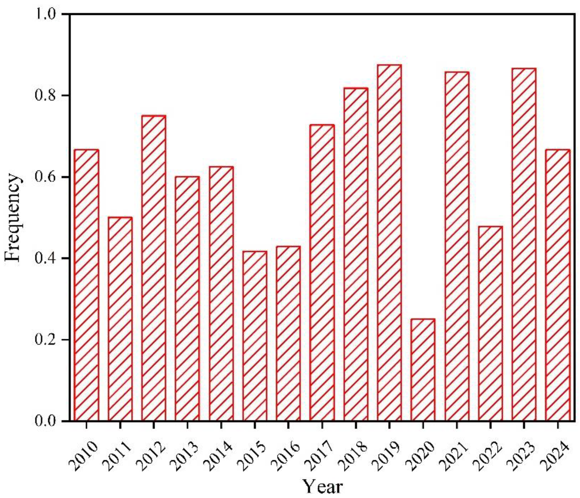
We counted a total of 179 biogas accidents from 2010 to August 2024, and calculated the proportion of biogas poisoning and suffocation accidents to the total number of accidents each year, as shown in Figure 3. This paper used the frequency distribution of biogas poisoning and suffocation accidents in the past 15 years as the accident frequency corresponding to the input variable in the Bayesian neural network model to perform deep learning.

(3)

Choose prior distribution.

It was necessary to select a suitable prior distribution for the weights and biases of the above-designed network. This paper used a Gaussian distribution.

(4)

Divide the training set and test set.

Random sampling was performed on the total data, and 20% of the data was used as the test set in this model.

(5)

Train the network and get predictions.

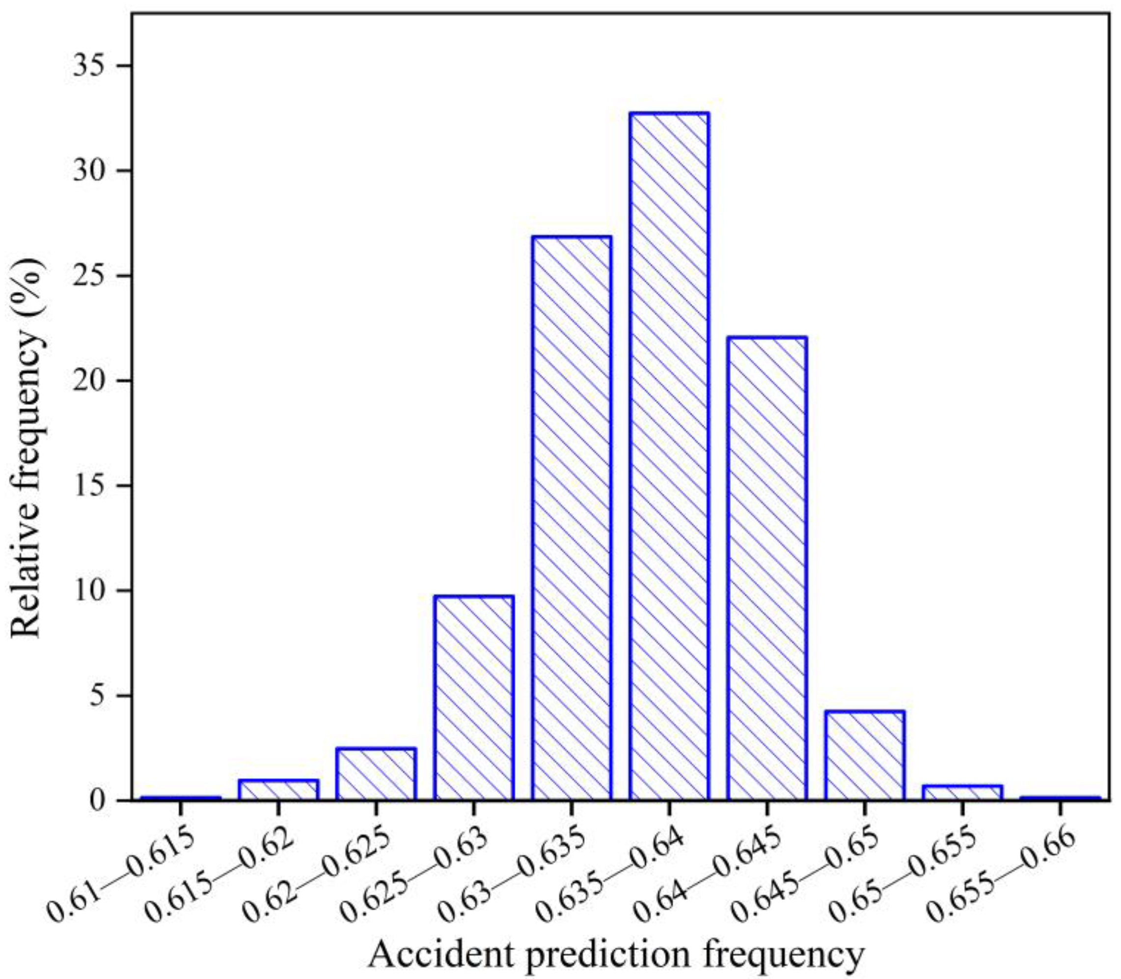
The network model was trained using the Bayesian method. In this paper, the Markov Chain Monte Carlo method (MCMC) was used to determine the posterior probability distribution, and then weighted samples were extracted from the posterior distribution to predict the results. The results are shown in Figure 4.

(6)

Model Evaluation.

The mean squared error (MSE) was used to evaluate the performance of the Bayesian neural network model. The mean squared error was an indicator to measure the difference between the model prediction value and the actual observation value. The smaller the mean square error, the higher the prediction accuracy of the model. The mean square error of the Bayesian neural network model designed in this paper was MSE = 0.0012. The confidence probability of the model is 0.942.

From the prediction results, we can see that the frequency range of biogas poisoning and suffocation accidents predicted by the Bayesian neural network was 0.610–0.660, the probability that the accident frequency falls between 0.635–0.640 was 32.73%, the probability that the accident frequency falls between 0.630–0.635 was 26.85%, the probability that the accident frequency falls between 0.640–0.645 was 22.05%, and the probability of falling in other frequency ranges was less than 10%. This indicated that the predicted frequency of biogas poisoning and suffocation accidents was concentrated between 0.630 and 0.645.

Trávníček et al. counted 208 biogas accidents in Europe (mainly Germany) from 2006 to 2016, among which the frequency of biogas poisoning and suffocation accidents was only 3% [24]. From the frequency statistics of biogas poisoning and suffocation accidents from 2010 to August 2024, it can be seen that the highest frequency of poisoning and suffocation accidents in these 15 years reached 0.875, and the lowest accident frequency was 0.25. The frequency of poisoning and suffocation accidents predicted by the Bayesian neural network model was also above 0.6. This shows that it was crucial to reduce the frequency of biogas poisoning and suffocation accidents in China. The prevention of biogas poisoning and suffocation accidents in pre-treatment pools can be started from three aspects: first, ensure the ventilation effect to prevent toxic and harmful gases from exceeding the standard; second, strengthen the management of confined space operations, and strictly follow the requirements of ‘ventilation first, then testing, finally operation’; third, strictly implement protection requirements to ensure the safety of operators themselves and avoid blind rescue.

3.4. Simulation of Biogas Diffusion in Pre-Treatment Pool

Considering that it is difficult to restore the real scene of biogas poisoning and suffocation accidents, this paper used FLUENT16.0 to simulate the biogas diffusion scene in the pre-treatment pool workshop, which strives to reproduce the real scene to the greatest extent and provide practical measures for preventing and controlling biogas poisoning and suffocation accidents.

3.4.1. Biogas Diffusion Under Free Ventilation

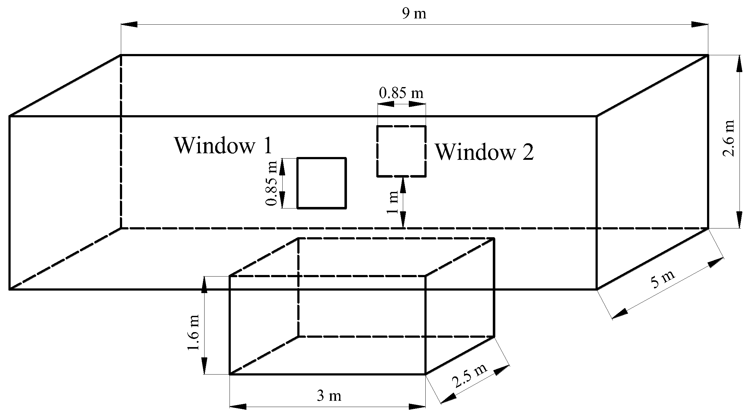
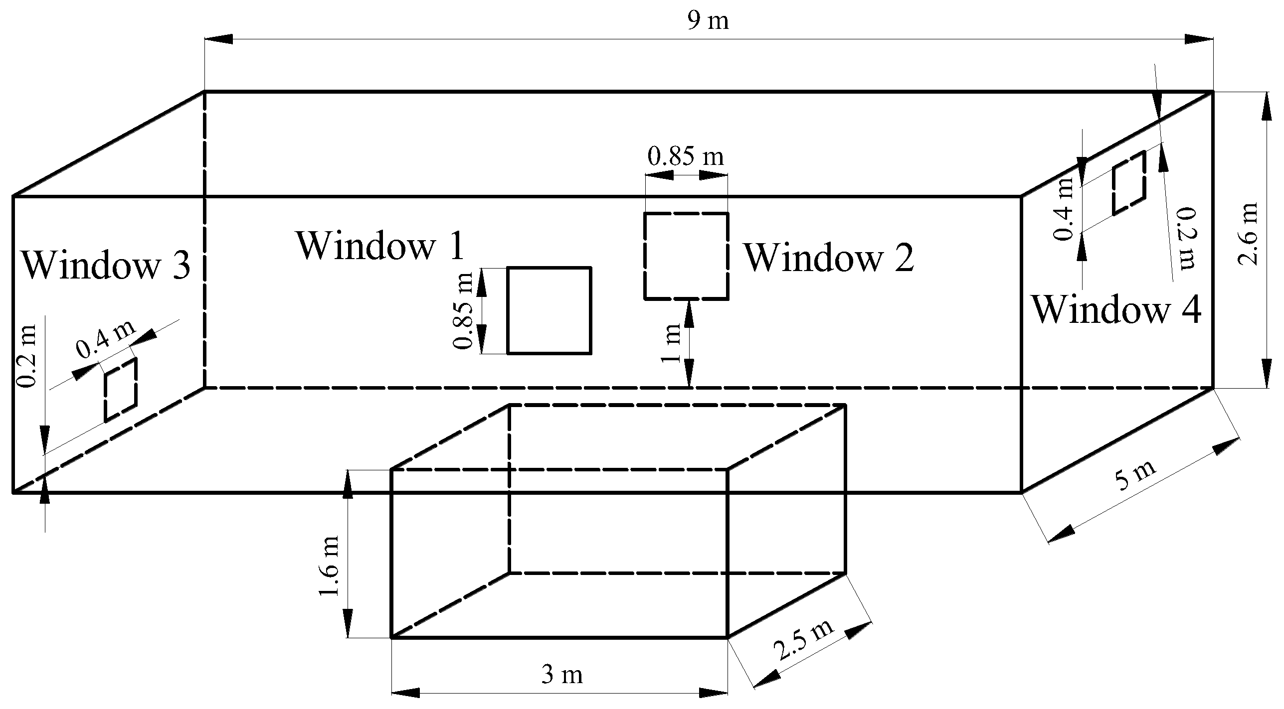
The ground space size of the workshop was 9 m × 5 m × 2.6 m. In the middle of the workshop, there was a 3 m × 2.5 m × 3.2 m pit-type pre-treatment pool, and the liquid level was 1.6 m. The air temperature in the workshop was 33 °C.

(1)

Establish the pre-treatment pool workshop model.

The space above the liquid surface of the pre-treatment pool was defined as the fluid simulation area, and the center of the horizontal plane of the workshop was considered the origin. The X-axis value of the overall fluid domain was between 0 m and 9 m, the Y-axis value was between 0 m and 5 m, and the Z-axis value was between −1.6 m and 2.6 m. The size of the two windows was 0.85 m × 0.85 m, and both were 1 m above the ground. The model is shown in Figure 5.

(2)

Boundary conditions.

The manure fermentation in the pre-treatment pool workshop produces biogas. According to the staff working in the biogas plant, the composition and proportion of the biogas produced in the pre-treatment pool were as follows: methane 3–5%, carbon dioxide 10–25%, hydrogen sulfide 0.03–0.5%. For this simulation, the components of biogas produced in the pre-treatment pool were 4% methane, 17.5% carbon dioxide, and 0.5% hydrogen sulfide, and the gas production rate was 0.1 m/s.

To simulate the diffusion of biogas under natural ventilation, it is necessary to set the wind speed of the window. This paper used the average wind speed of 2.94 m/s in 2023 in the city where the biogas station was located as the wind speed of the air inlet window (window 1), and the other window (window 2) as the outlet. Note that the air flew through the air inlet window.

The biogas diffusion process in the pre-treatment pool workshop was simulated for 1000 s with a data sampling time interval of 1 s.

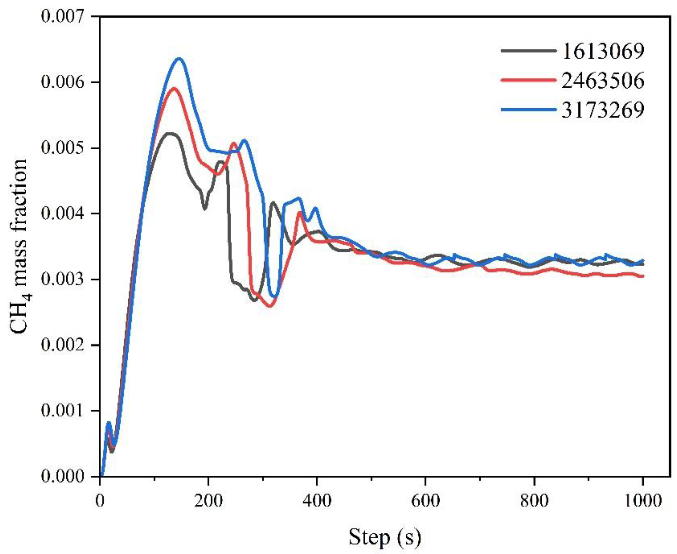
(3)

Grid-independent verification

Verification of independent verification in a simulation is an important part of ensuring the accuracy and reliability of numerical simulation results. This study divided three groups of independent grid parameters, and the number of grids (Elements) was 1,613,069, 2,463,506 and 3,173,269, respectively.

The average element quality of the three groups meshing was more than 0.8, indicating that the overall quality of the meshing was high.

The CH₄ mass fraction at the point (0, 0, 2.40) was selected as the monitoring point, and the simulation values obtained from the three groups meshing were compared. Figure 6 shows the CH₄ mass fraction at the same point in three groups, and the final equilibrium values were relatively close. Therefore, from the perspective of accuracy and efficiency, the number of grids for this simulation was selected as 1,613,069.

(4)

Simulation Results.

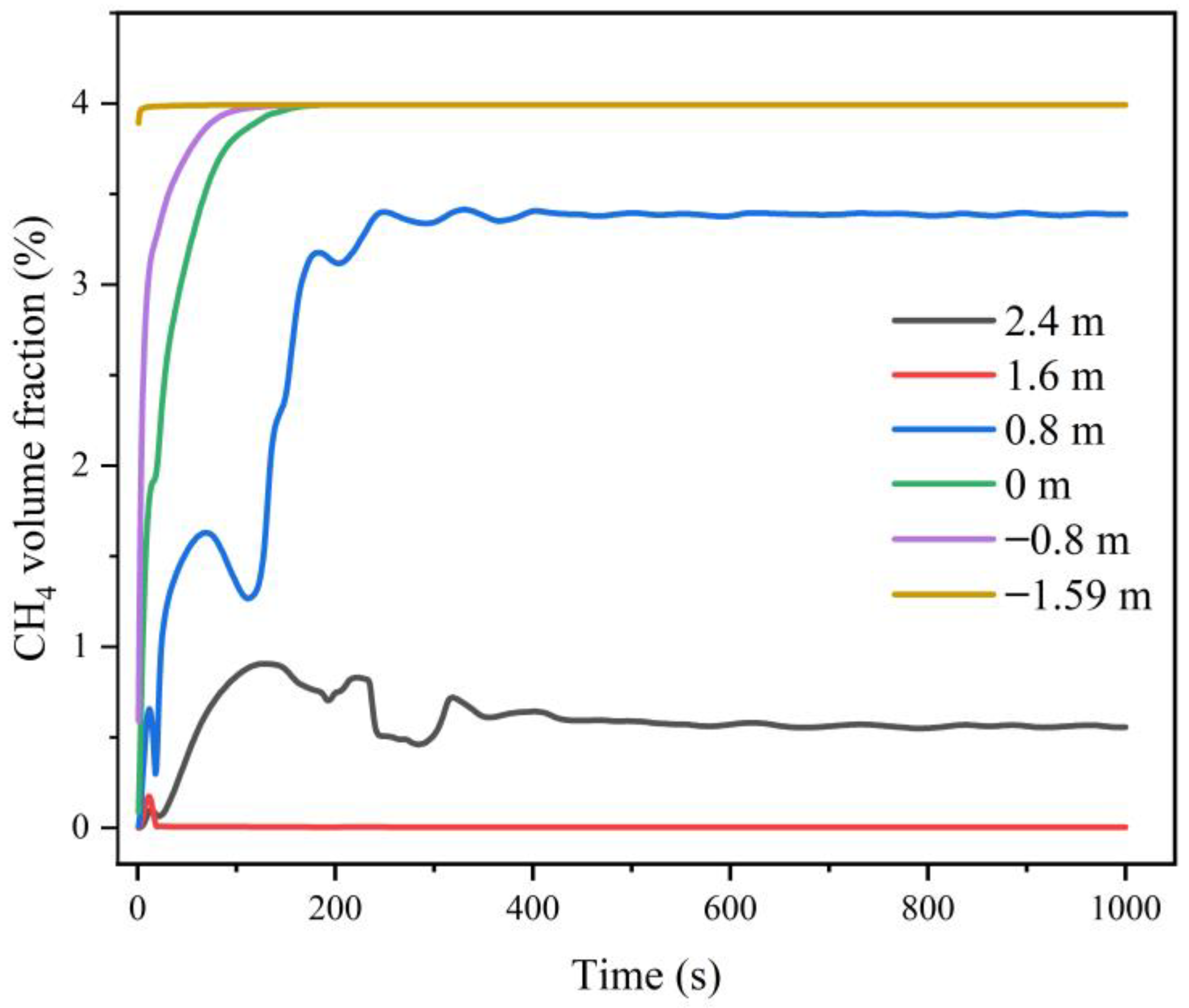
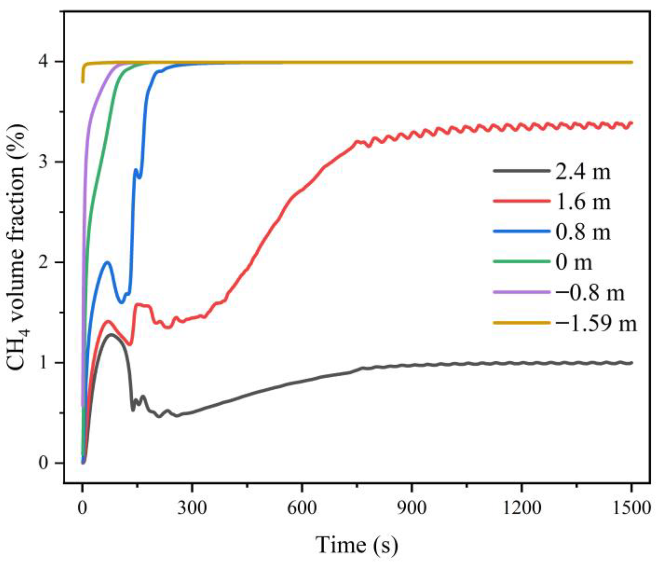
Methane, carbon dioxide and hydrogen sulfide gases were detected at 6 points, which were (0, 0, −1.59), (0, 0, −0.80), (0, 0, 0), (0, 0, 0.80), (0, 0, 1.60) and (0, 0, 2.40).

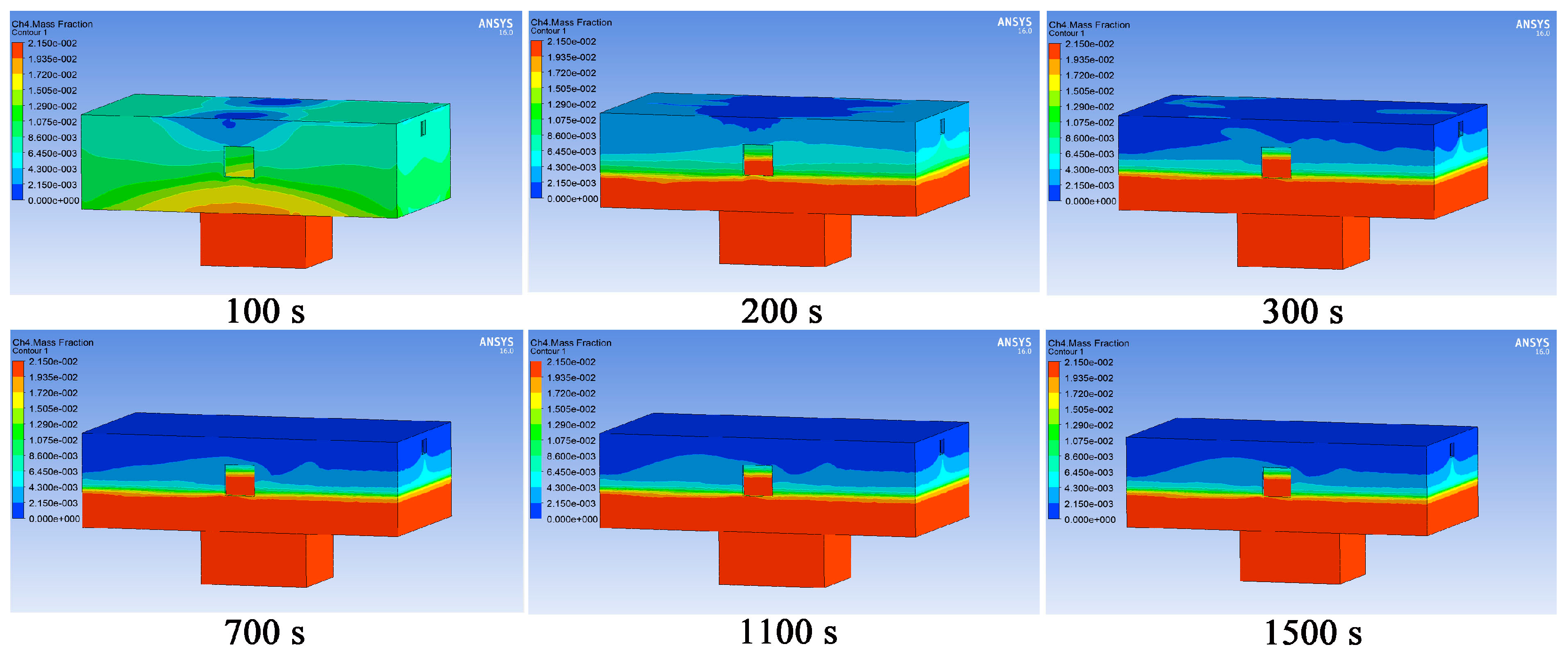
Figure 7 shows the changes in methane gas volume fraction at six monitoring points. The methane gas concentration values at the six monitoring points all reached equilibrium at around 320 s. When Z = −1.59 m, −0.80 m and 0 m, the maximum equilibrium value of the volume fraction of methane gas was 3.99%. When Z = 0.80 m, the equilibrium value of the volume fraction of methane gas was 3.39%. Considering that the explosion limit of methane is 5–15%, the methane gas concentrations at the above four points were close to the lower explosion limit. When Z = 1.60 m and 2.40 m, the equilibrium values of the volume fraction of methane gas were 0.0033% and 0.55%, respectively.

When Z = 1.60 m, the volume fraction of methane gas was the smallest. This was because there was a 0.85 m × 0.85 m window 1 m above the ground. Under natural ventilation (wind speed was 2.94 m/s), there was less methane gas there. The other five points were not within the window height range, so the volume fraction of methane gas was higher.

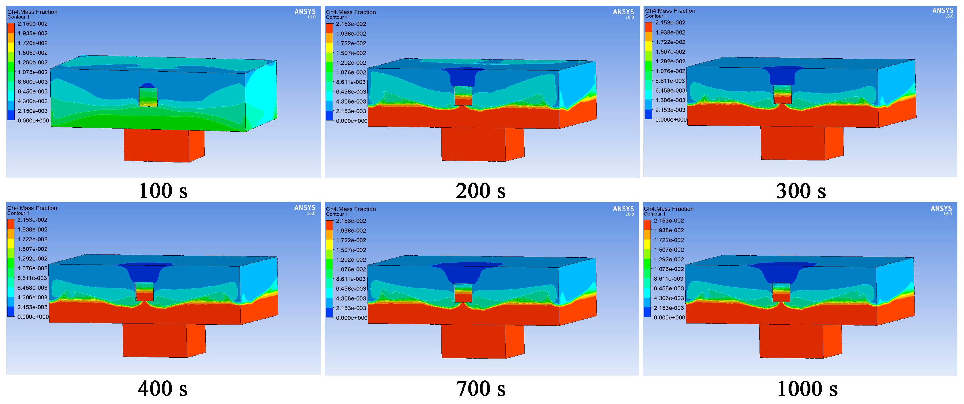
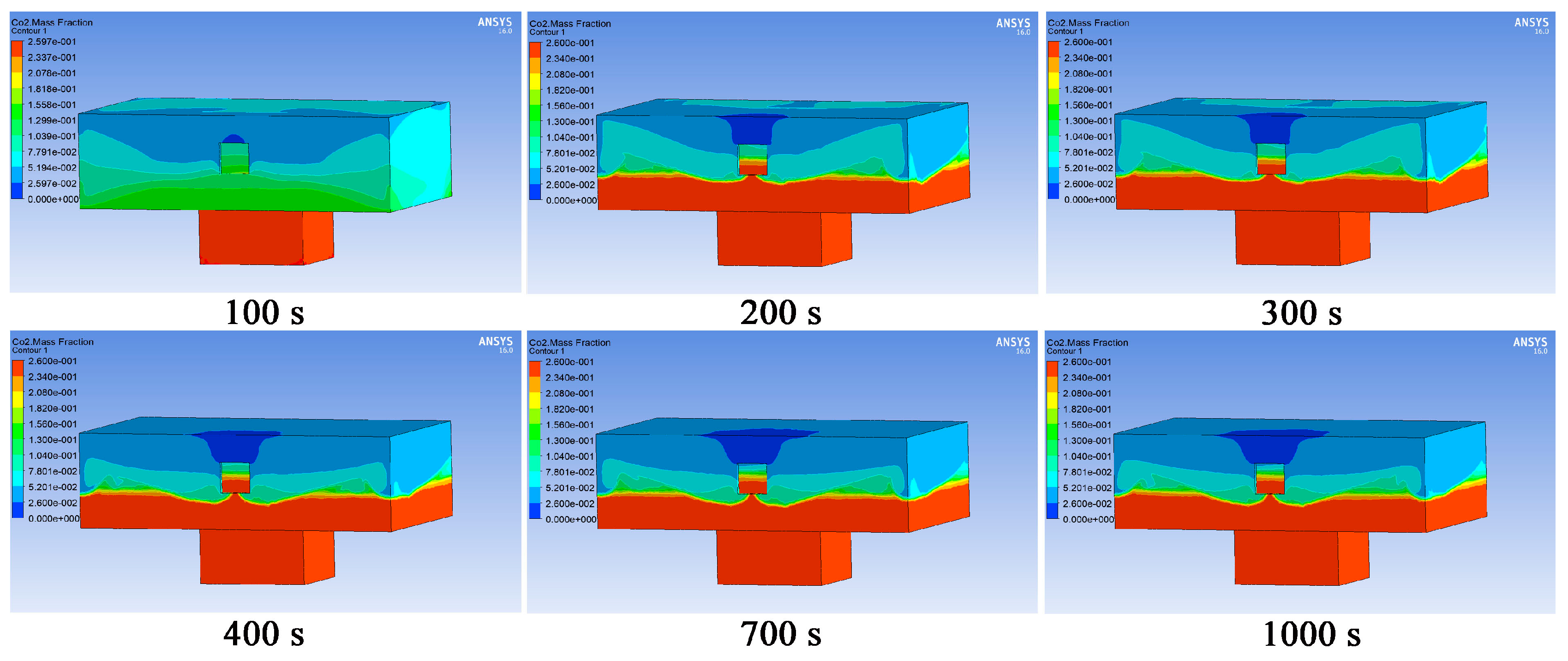
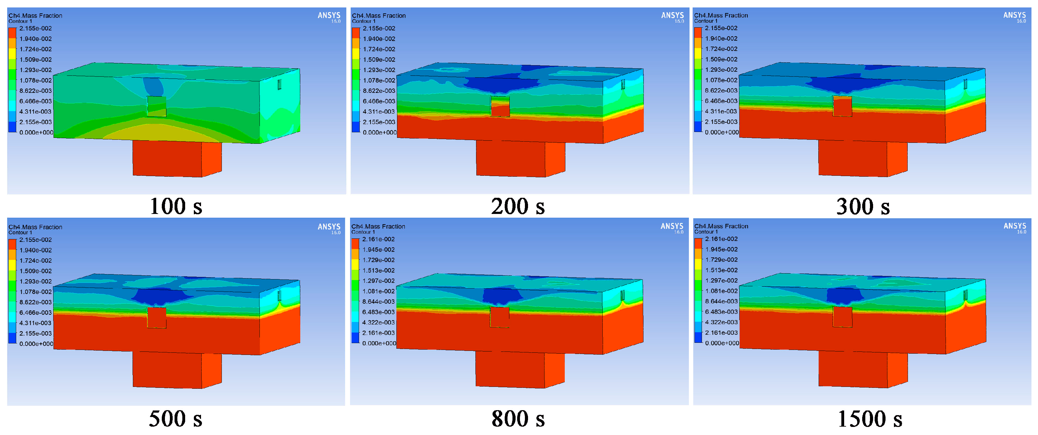
Figure 8 presents the distribution of methane gas concentration at different time points. As shown in Figure 8, the air entering through natural ventilation diluted the methane gas in the area above 0.8 m in the z-axis direction, while the methane gas in the area below was not diluted.

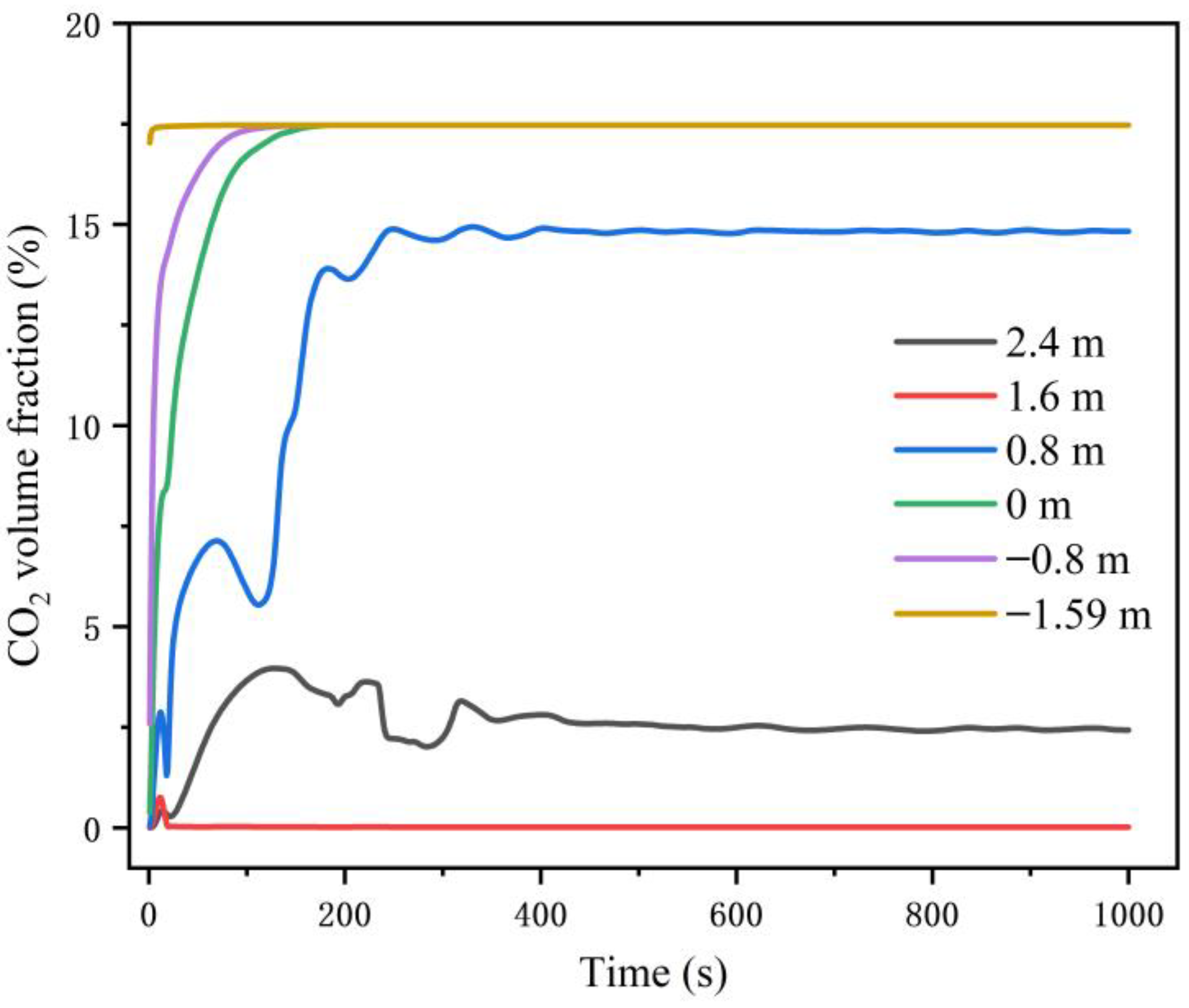
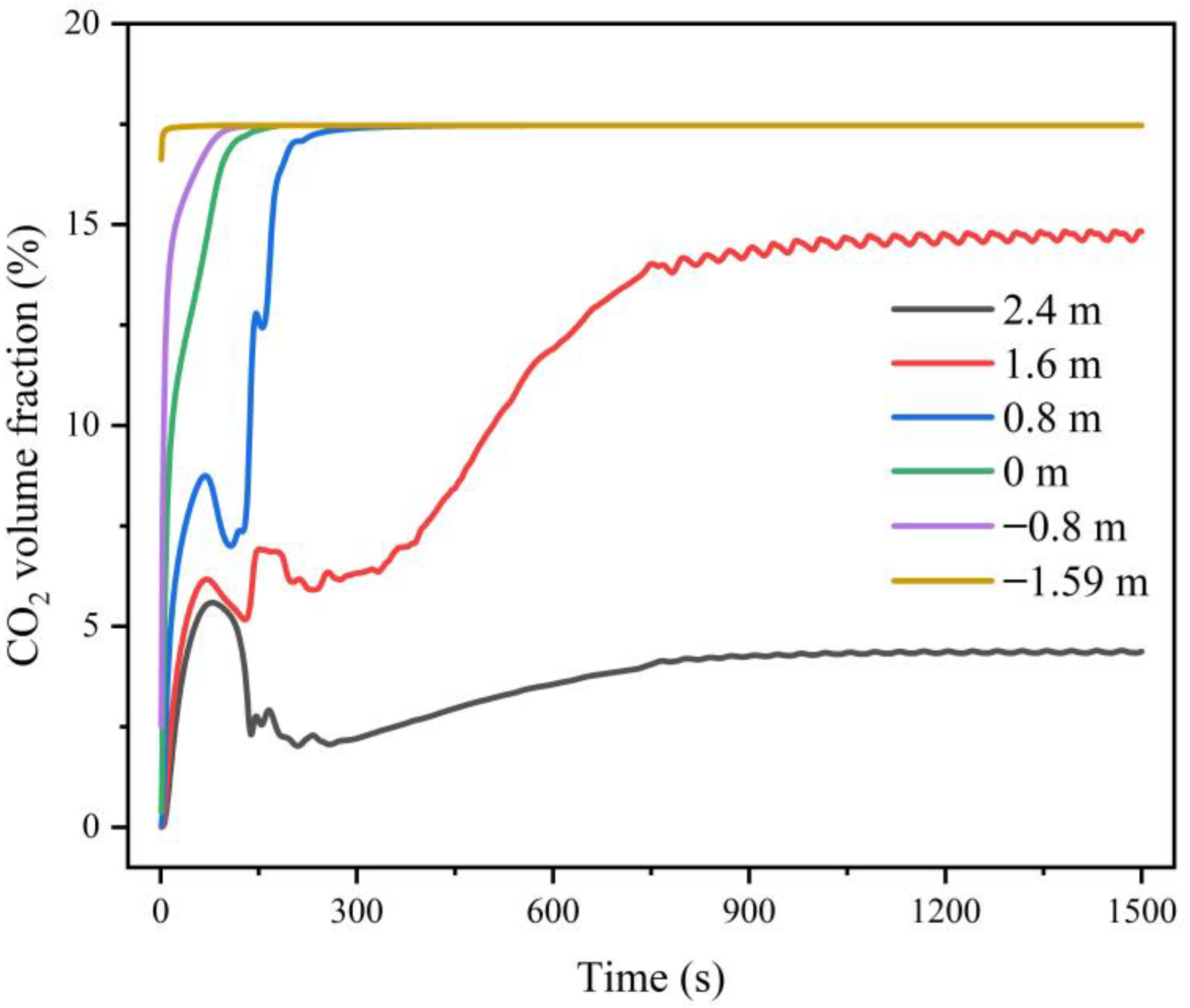
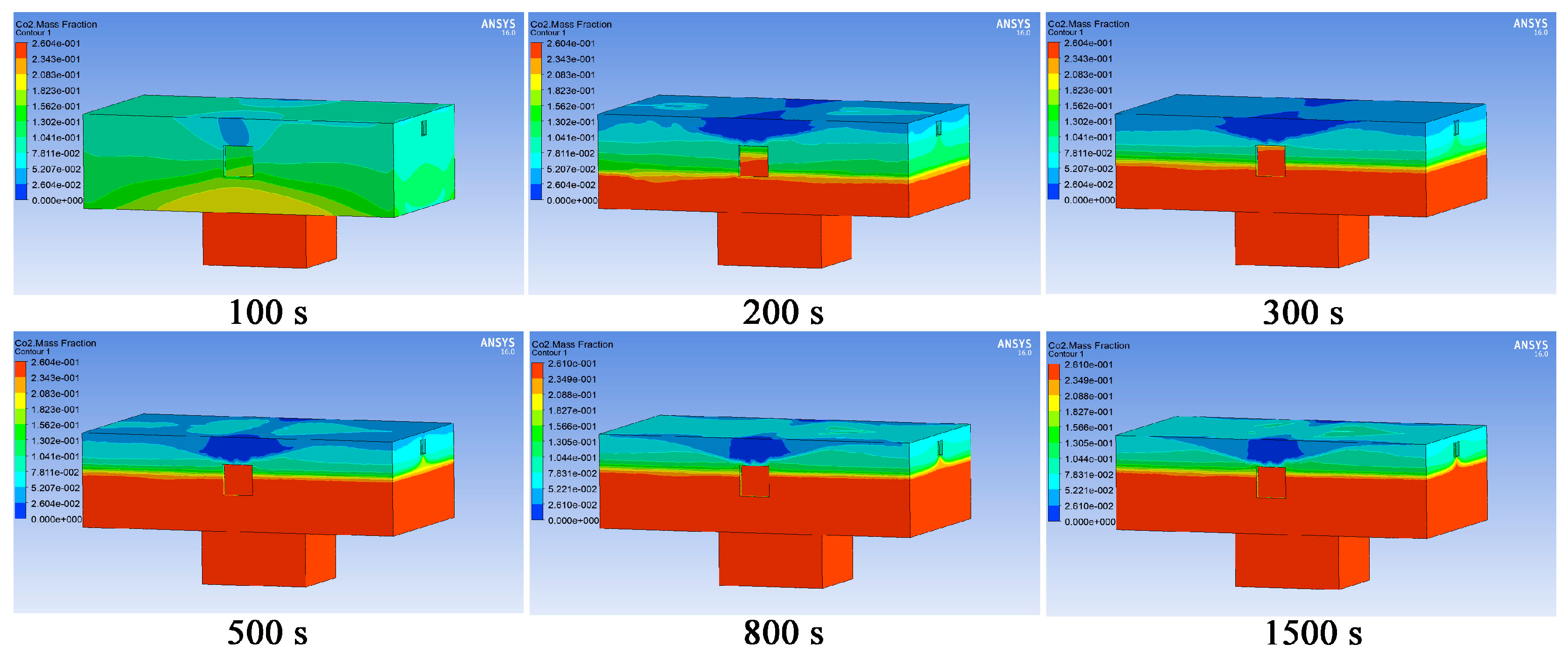
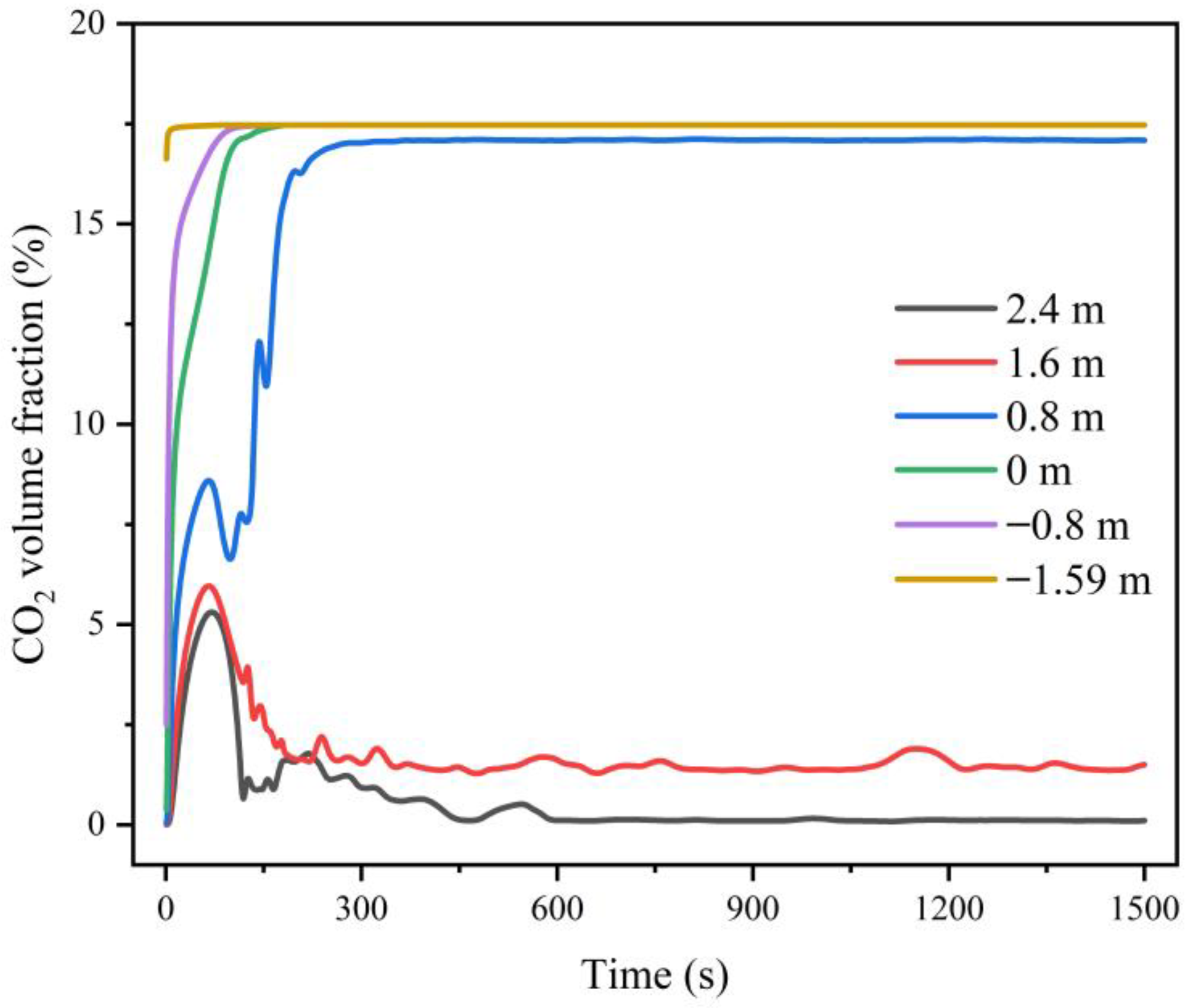
Figure 9 shows the changes in the volume fraction of carbon dioxide gas at the six monitoring points. The carbon dioxide concentration values at the six monitoring points all reached equilibrium at around 400 s. When Z = −1.59 m, −0.80 m and 0 m, the volume fraction equilibrium value of carbon dioxide gas was 17.47%; when Z = 0.80 m, the volume fraction equilibrium value of carbon dioxide gas was 14.83%. Note that when the carbon dioxide concentration reaches 10%, people would lose consciousness or even stop breathing in less than 1 min. The equilibrium concentration of carbon dioxide at the above four points exceeded 10%. When Z = 1.60 m and 2.40 m, the equilibrium values of the volume fraction of carbon dioxide gas were 0.014% and 2.43%, respectively. 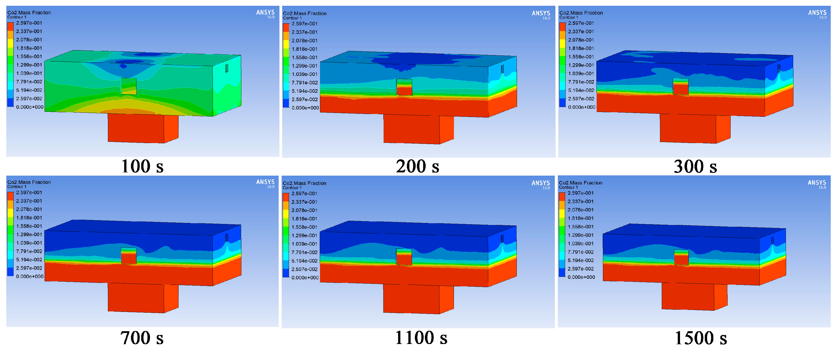Figure 10 presents the distribution of carbon dioxide gas concentration at different time points. As shown in Figure 10, the air entering through natural ventilation diluted the carbon dioxide gas in the area above 0.8 m in the z-axis direction, while the carbon dioxide gas in the area below was not diluted.

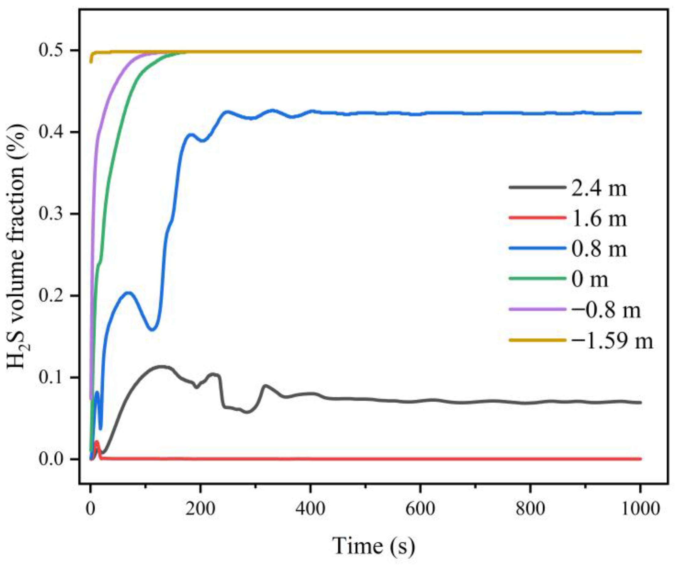
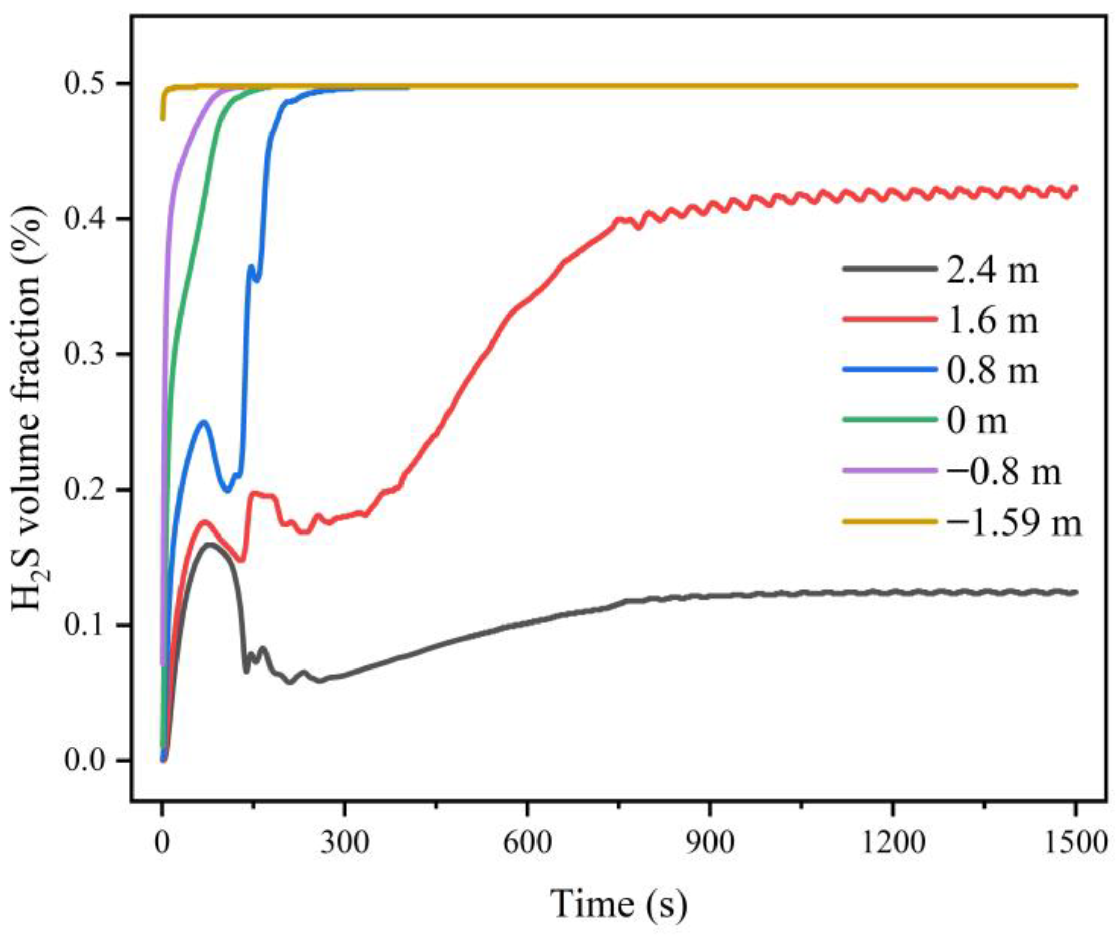
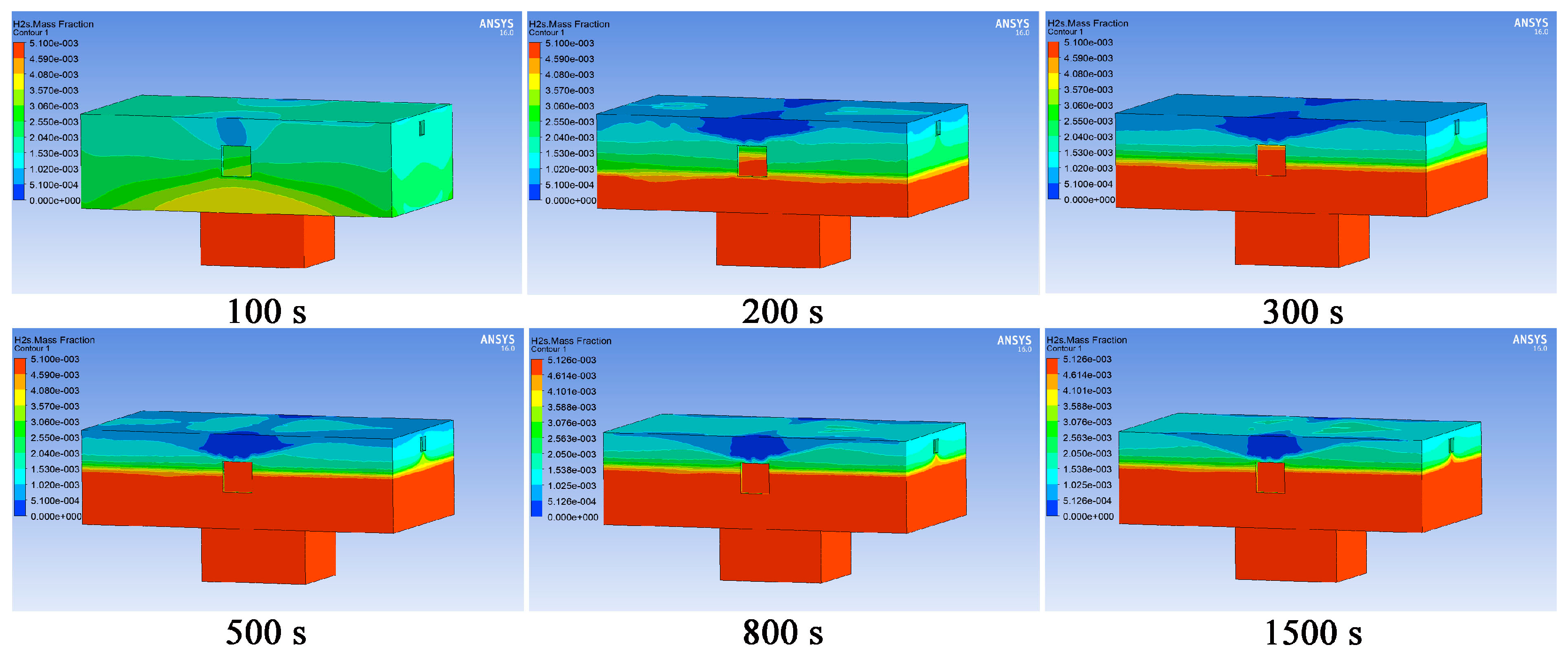
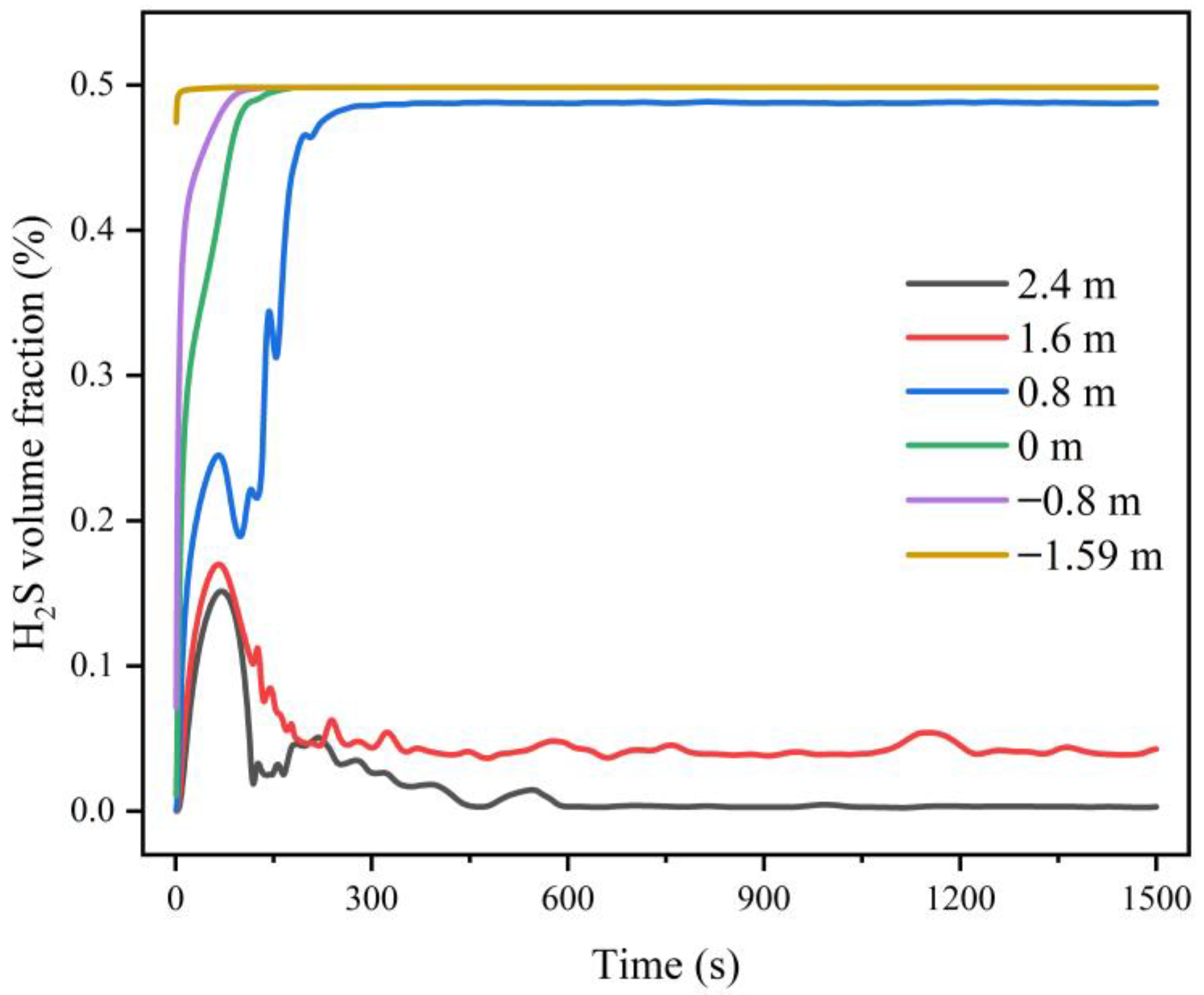
Figure 11 shows the changes in the volume fraction of hydrogen sulfide gas at the six monitoring points. The hydrogen sulfide gas concentration values at the six monitoring points all reached equilibrium at around 400 s. When Z = −1.59 m, −0.80 m and 0 m, the volume fraction equilibrium value of hydrogen sulfide gas was 0.49%; when Z = 0.80 m, the volume fraction equilibrium value of hydrogen sulfide gas was 0.42%. Note that when the concentration of hydrogen sulfide reached 0.1%, people would die immediately. The results showed that the concentration of hydrogen sulfide gas at the above four points exceeded its lethal concentration. When Z = 1.60 m and 2.40 m, the equilibrium values of the volume fraction of hydrogen sulfide gas were 0.000412% and 0.069%, respectively.

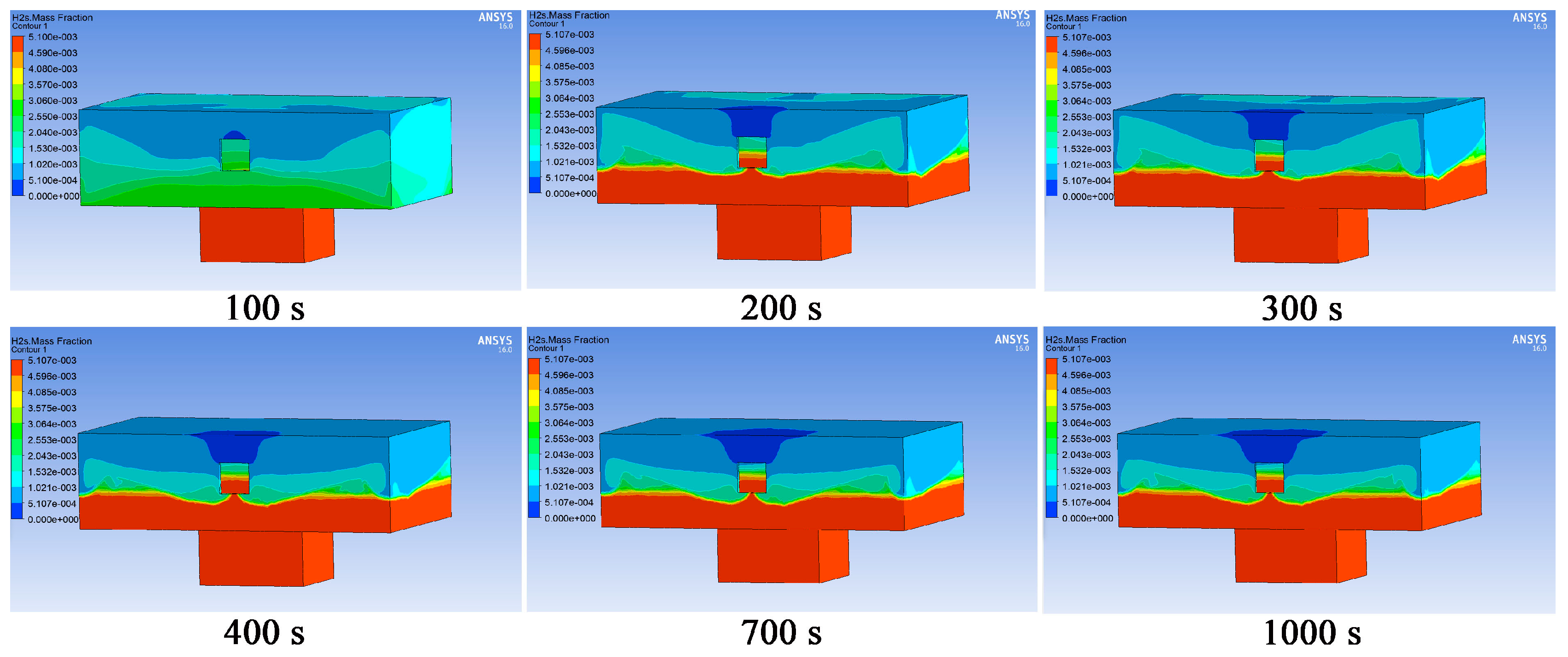
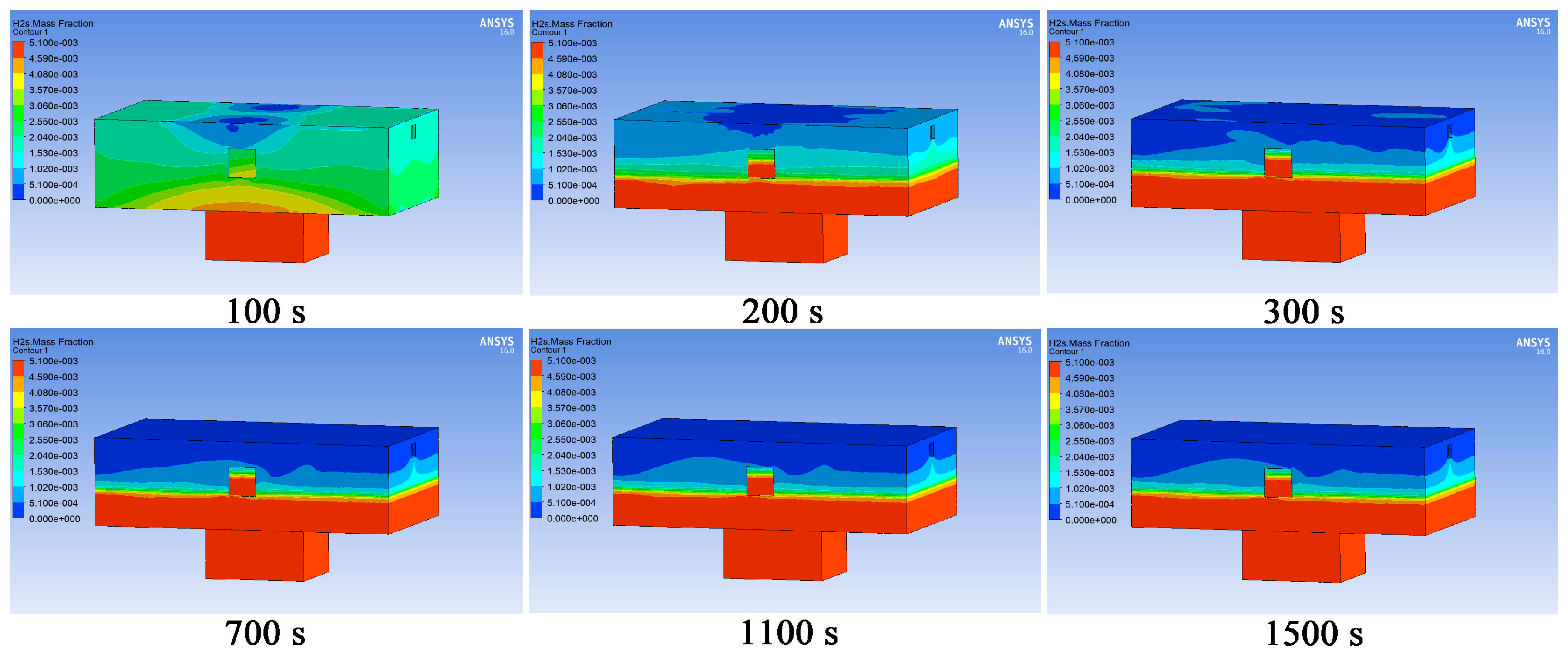
Figure 12 presents the distribution of hydrogen sulfide gas concentration at different time points. The air entering through natural ventilation diluted the hydrogen sulfide gas in the area 0.8 m and above on the z-axis direction, while the hydrogen sulfide gas in the area below was not diluted.

3.4.2. Diffusion of Biogas Under Forced Ventilation (6 Times/h)

It can be seen from the natural ventilation simulation results that natural ventilation can dilute the concentration to a certain extent, but the disadvantage of natural ventilation is that the wind speed conditions are unstable. If there was no wind or the wind speed was low, higher concentrations of toxic and harmful gases would easily accumulate in the pre-treatment pool workshop. It can be seen from criterion item 13.9 of ‘Technical Specifications for Biogas Engineering Part 1: Engineering Design NY/T 1220.1-2019’ that when natural ventilation cannot meet the requirements, forced ventilation can be used.

(1)

Establish the model.

In accordance with the requirements for the number and area of vents in the standard specifications, two vents were added to the natural ventilation simulation model. The size of the two windows was 0.4 m × 0.4 m. The vent close to the ground was 0.2 m away from the ground, and the other vent close to the roof was 0.2 m away from the roof. The model is shown in Figure 13.

(2)

Grid meshing.

The number of simulation grids was 1,611,141, and the average element quality was 0.84, which indicated that the overall grid quality was high.

(3)

Boundary conditions.

According to criterion item 13.9 of ‘Technical Specifications for Biogas Engineering Part 1: Engineering Design NY/T 1220.1-2019’, the number of forced ventilation frequencies was set at 6 times/h. According to criterion item 6.3.9 of the ‘Design Code for Heating, Ventilation and Air Conditioning of Industrial Buildings GB50019-2015’, this simulation discharged 2/3 of the total exhaust volume from the lower vent and 1/3 of the total exhaust volume from the upper vent. Specifically, two windows (window 1 and window 2) were used as air inlets, and the calculated speed was 0.1487 m/s. Window 3 was used as the air outlet, and the exhaust volume accounted for two-thirds of the total exhaust volume. Window 4 was used as the air outlet, and the exhaust volume accounted for one-third of the total exhaust volume. The biogas diffusion rate and composition ratio referred to the natural ventilation simulation parameters. The biogas diffusion process in the pre-treatment pool workshop was simulated for 1500 s with a data sampling time interval of 1 s.

(4)

Simulation results.

Figure 14 shows the changes in methane gas volume fraction at six monitoring points. As shown in Figure 14, the methane gas concentration values at the six monitoring points all reached equilibrium at around 700 s. When Z = −1.59 m, −0.80 m, 0 m, and 0.80 m, the volume fraction equilibrium value of methane gas was 3.99%, which had reached 80% of the lower explosion limit of methane; when Z = 1.60 m, the volume fraction equilibrium value of methane gas was 3.39%, which had reached 68% of the lower explosion limit of methane; when Z = 2.40 m, the volume fraction equilibrium value of methane gas was 0.99%, which had reached 20% of the lower explosion limit of methane.

Figure 15 demonstrates the distribution of methane gas concentration at different time points. As shown in Figure 15, forced ventilation (6 times/h) diluted the methane gas in the area above 1.6 m in the z-axis direction, while the methane gas in the area below was not diluted.

Figure 16 exhibits the changes in carbon dioxide gas volume fraction at the six monitoring points. As shown in Figure 16, the carbon dioxide gas concentration values at the six monitoring points all reached equilibrium at around 700 s. When Z = −1.59 m, −0.80 m, 0 m, and 0.8 m, the volume fraction equilibrium value of carbon dioxide gas was 17.47%; when Z = 1.60 m, the volume fraction equilibrium value of carbon dioxide gas was 14.82%; when Z = 2.40 m, the volume fraction equilibrium value of carbon dioxide gas was 4.37%. Except for the top area of the workshop, the carbon dioxide concentration in other areas was far above the lethal concentration.

Figure 17 presents the distribution of carbon dioxide gas concentration at different time points. As shown in Figure 17, forced ventilation (6 times/h) diluted the carbon dioxide gas in the area above 1.6 m in the z-axis direction, while the carbon dioxide gas in the area below was not diluted.

Figure 18 shows the changes in the volume fraction of hydrogen sulfide gas at the six monitoring points. As shown in Figure 18, the hydrogen sulfide gas concentration values at the six monitoring points all reached equilibrium at around 700 s. When Z = −1.59 m, −0.80 m, 0 m, and 0.8 m, the volume fraction equilibrium value of hydrogen sulfide gas was 0.49%; when Z = 1.60 m, the volume fraction equilibrium value of hydrogen sulfide gas was 0.42%; when Z = 2.40 m, the volume fraction equilibrium value of hydrogen sulfide gas was 0.12%. The hydrogen sulfide concentration in all areas of the workshop was far above the lethal concentration.

Figure 19 exhibits the distribution of hydrogen sulfide gas concentration at different time points. Although the concentration of hydrogen sulfide in the area near the top of the workshop was lower than that in other areas, the concentration of hydrogen sulfide in the entire workshop would cause the death of workers.

3.4.3. Biogas Diffusion Under the Combination of Forced Ventilation and Emergency Exhaust Fan

From the simulation results of forced ventilation (6 times/h), it can be seen that the methane gas concentration in the pre-treatment pool workshop was close to the lower explosion limit, the carbon dioxide concentration was far beyond the lethal concentration except at the top area of the workshop, and the hydrogen sulfide concentration exceeded the lethal concentration in the entire workshop, so forced ventilation (6 times/h) did not meet the requirements.

According to criterion item 4.8.1 of the ‘Technical Specifications for Large and Medium-sized biogas plants GB51063-2014’, when the methane concentration in the air is detected to reach 20% (volume ratio) of the lower explosion limit, the emergency exhaust fan should be able to open automatically. Considering that the ventilation frequency of the emergency exhaust fan should not be less than 6 times/h, this section is simulated based on the forced ventilation (6 times/h) in the previous section and added the emergency exhaust fan. We assumed that the emergency exhaust fan had a ventilation frequency of 6 times/h.

Two windows (window 1 and window 2) were used as air inlets, and the wind speed was set to 0.2974 m/s. In addition, window 3 was used as the air outlet, and the exhaust volume accounted for two-thirds of the total exhaust volume. Window 4 was used as the air outlet, and the exhaust volume accounted for one-third of the total exhaust volume. The biogas diffusion rate and component ratio referred to the simulation parameters in the previous section.

We simulated the biogas diffusion process in the pre-treatment pool workshop for 1500 s with a data sampling time interval of 1 s.

Figure 20 indicates the changes in methane gas volume fraction at six monitoring points.

As shown in Figure 20, the methane gas concentration values at the six monitoring points all reached equilibrium at around 300 s. When Z = −1.59 m, −0.80 m, 0 m, and 0.80 m, the volume fraction equilibrium value of methane gas was 3.99%, which had reached 80% of the lower explosion limit of methane; when Z = 1.60 m, the volume fraction equilibrium value of methane gas was 0.34%; when Z = 2.40 m, the volume fraction equilibrium value of methane gas reached 0.024%. The methane concentration in the area 0.8 m and below on the z-axis direction was close to the lower explosion limit, and the methane concentration in the area above had not yet reached 20% of the lower explosion limit.

Figure 21 displays the distribution of methane gas concentration at different time points. As shown in Figure 21, the combined effect of forced ventilation and emergency exhaust fans diluted the methane gas in the area 1 m and above on the z-axis direction, while the methane gas in the area below 1 m was not diluted.

Figure 22 revealed the changes in the volume fraction of carbon dioxide gas at the six monitoring points. According to Figure 22, the carbon dioxide gas concentration values at the six monitoring points all reached equilibrium at around 300 s. When Z = −1.59 m, −0.80 m, 0 m, and 0.8 m, the volume fraction equilibrium value of carbon dioxide gas was about 17%. The carbon dioxide concentration at the above four points exceeded the lethal concentration of carbon dioxide. When Z = 1.60 m, the volume fraction equilibrium value of carbon dioxide gas was 1.49%; when Z = 2.40 m, the volume fraction equilibrium value of carbon dioxide gas reached 0.10%.

Figure 23 demonstrates the distribution of carbon dioxide gas concentration at different time points. As shown in Figure 23, the combined action of forced ventilation and the emergency exhaust fan diluted the carbon dioxide gas in the area above 1 m in the z-axis direction, while the carbon dioxide gas in the area below 1 m was not diluted.

Figure 24 displays the changes in the volume fraction of hydrogen sulfide gas at the six monitoring points. As shown in Figure 24, the hydrogen sulfide gas concentration values at the six monitoring points all reached equilibrium at around 300 s. When Z = −1.59 m, −0.80 m, 0 m, and 0.8 m, the volume fraction equilibrium value of hydrogen sulfide gas was 0.49%, which was far higher than the lethal concentration 0.1%; when Z = 1.60 m, the volume fraction equilibrium value of hydrogen sulfide gas was 0.043%, which would cause death in 15–60 min; when Z = 2.40 m, the volume fraction equilibrium value of hydrogen sulfide gas reached 0.003%, which would not pose a threat to the life or health of personnel.

Figure 25 indicates the distribution of hydrogen sulfide gas concentration at different time points. As shown in Figure 25, the combined action of forced ventilation and the emergency exhaust fan diluted the hydrogen sulfide gas in the area above 1 m in the z-axis direction, while the hydrogen sulfide gas in the area below 1 m was not diluted.

3.5. Simulation Results Analysis

According to on-site investigations in biogas plants, some plants usually choose natural ventilation for pre-treatment pool workshop. However, due to the unstable wind speed of natural ventilation, natural ventilation obviously cannot satisfy the requirements for the pre-treatment pool workshop, a place with a high incidence of poisoning and suffocation accidents. This reflected the importance and urgency of setting up forced ventilation and emergency exhaust. It can be seen from the simulation results that setting up forced ventilation and emergency exhaust can dilute the concentrations of methane, carbon dioxide and hydrogen sulfide to a certain extent. Assuming that the height of the operators is between 1.6 m and 1.8 m, under the condition of forced ventilation and emergency ventilation in the pre-treatment pool workshop, when operators enter the workshop, the concentration of methane gas and carbon dioxide gas in the area 1.6 m and above on the z-axis direction would not bring explosion and suffocation risks. However, under the same conditions, there existed risks of methane gas explosion and carbon dioxide suffocation through forced ventilation alone. For hydrogen sulfide, under the combined effect of forced ventilation and emergency exhaust, the gas concentration in the area 1.6 m and above on the z-axis direction was greatly reduced, but it would still cause harm to the lives of workers. The reason for the above situation was that the proportion of hydrogen sulfide in biogas is generally 0.03–0.5%, the ANSYS Fluent simulation determined its proportion based on the maximum value considering that hydrogen sulfide itself is a highly toxic substance. Therefore, the concentration of hydrogen sulfide gas in the simulation result was relatively high. In addition, the ventilation times in this simulation were determined according to the minimum requirements in the standard specifications, aiming to explore the diffusion law of biogas and prove the necessity of setting up forced ventilation and emergency exhaust fan. At the same time, enterprises are also encouraged to use numerical simulation methods to determine ventilation types and optimal air exchange times that are more in line with actual conditions.

Criterion item 4.8.1 of the ‘Technical Specifications for Large and Medium-sized biogas plants GBT51063-2014’ stipulates that the emergency exhaust fan should be automatically turned on when the methane concentration reaches 20% of the lower explosion limit (methane concentration (volume ratio) reaches 1%). According to the relevant provisions of the industry standard ‘Technical Regulations for Urban Gas Alarm Control Systems CJJ/T146’, the installation location of the methane concentration alarm should be no more than 0.3 m away from the roof. According to the above installation location standards, the installation height of the methane concentration alarm in the pre-treatment pool workshop should be between 2.3–2.6 m. We assumed that the methane alarm in the pre-treatment pool workshop was installed at position Z = 2.4 m. From the simulation results, we can see that the methane gas concentration was between 3% and 4% when Z = −1.59 m, −0.80 m, 0 m, and 0.80 m, and this concentration range was close to the lower explosion limit of methane gas. However, the gas concentration at the installation location of the methane alarm (Z = 2.4 m) was less than or close to 1%. If operators work near the pre-treatment pool, the methane gas concentration is close to the lower explosion limit, so there is a risk of explosion. However, the concentration monitored by the methane gas alarm had not yet reached the standard for initiating emergency exhaust ventilation. This reflected the problem of unreasonable installation of methane alarm. Through the above analysis, the corresponding control measures proposed in this paper were that methane gas alarms should be installed in high-frequency working areas of operators and interlocked with emergency exhaust fans.

When Z = −1.59 m, −0.80 m, 0 m, and 0.80 m, the three ventilation methods had no obvious dilution effect on carbon dioxide and hydrogen sulfide gases in this area, and the equilibrium concentrations of the two gases exceeded the lethal concentration. Due to the high toxicity of hydrogen sulfide and its obvious odor, some studies and accident investigation reports believe that biogas poisoning and suffocation accidents are caused by hydrogen sulfide and, thus, ignore the colorless and odorless carbon dioxide gas which can easily cause suffocation of workers. There are three main reasons why carbon dioxide should not be ignored in biogas poisoning and suffocation accidents: First, from the simulation results, when forced ventilation and emergency exhaust fans worked together, the carbon dioxide concentration in the area 0.8 m and below on the z-axis was as high as 17%, far exceeding its lethal concentration. If operators perform inspection and maintenance in this area, the risk of suffocation would increase. Second, during the fermentation process of the raw materials, carbon dioxide gas was produced first and then hydrogen sulfide gas. Carbon dioxide gas is already produced during the hydrolysis stage of the raw materials, and Carbon dioxide gas is also produced during the subsequent acid production and methane production stages. The production of hydrogen sulfide gas requires sulfate-reducing bacteria to use the intermediate products produced during the hydrolysis and acid production stages as electron donors to reduce sulfate to sulfide which then combines with hydrogen ions to form hydrogen sulfide. When the concentration of hydrogen sulfide reaches the solubility limit of the liquid, it overflows the liquid surface in the form of gas. Third, the production of carbon dioxide by fermentation of raw materials is not easily affected by the contents of specific elements, while the contents of sulfate in the raw materials directly determine the output of hydrogen sulfide gas. The output of hydrogen sulfide gas varies for different raw materials. In a word, the causative factor of biogas poisoning and suffocation accidents cannot be uniformly determined to be hydrogen sulfide gas.

The standards and specifications related to biogas plants require the installation of methane gas alarms and hydrogen sulfide gas alarms in places prone to biogas leakage, and only stipulate that the methane gas alarms should be interlocked with the emergency exhaust fans. This shows that the forced ventilation system and emergency exhaust fans required by the standards and specifications are set up to prevent the explosion of combustible gases. However, the content of methane, carbon dioxide and hydrogen sulfide in the biogas produced by the pre-treatment pool workshop was relatively low, and poisoning and suffocation accidents had become the main type of accidents. Therefore, the requirements in the standards and specifications were not reasonable for the pre-treatment pool workshop. Existing measures to prevent and control poisoning and suffocation accidents mostly focus on operators’ safety consciousness, such as consciously wearing protective equipment and entering the factory according to procedures. If the safety awareness of operators and the operating procedures cannot be guaranteed, the incidence of poisoning and suffocation accidents would remain high. Therefore, it is necessary to reduce the incidence of poisoning and suffocation accidents from the perspective of controlling the concentration of toxic and harmful gases. Since hydrogen sulfide cannot be regarded as the only harmful factor in poisoning and suffocation accidents in the above discussion, and excessive carbon dioxide gas concentration can also cause suffocation and death of workers, it is indispensable to add carbon dioxide gas alarms in the high-frequency operation areas of workers in the pre-treatment pool workshop and interlock the carbon dioxide gas alarms with the emergency exhaust fans. The ‘Confined Space Operation Safety Guidance Manual’ stipulates that the upper limit of carbon dioxide gas concentration during confined space operations is 0.98%. When the concentration of carbon dioxide gas exceeds 3%, people would experience symptoms such as increased heart rate and blood pressure. To take into account both the life of workers and the costs of the enterprise, the limit value of the carbon dioxide gas alarm should be set to 3%. When the carbon dioxide gas concentration in the pre-treatment pool workshop reaches 3%, the emergency exhaust fan should be started.

4. Conclusions

This paper proposed the Bow-Tie-QCA-Bayesian Neural Network-Consequence Simulation model to conduct a quantified analysis on the poisoning and suffocation risk of a pre-treatment pool workshop. The main conclusions were as follows:

(1)

Bow-tie was applied to find out the causes of biogas poisoning and suffocation accidents in the pre-treatment pool workshop.

(2)

The QCA method explored the accident cause combination paths in management.

(3)

The Bayesian neural network model predicted the distribution of accident frequency and provides model accuracy, thereby improving the reliability of the prediction results.

(4)

The ANSYS Fluent simulation quantified the biogas diffusion consequences in three different ventilation types.

(5)

The importance and necessity of ventilation and the reasons why the methane alarm was installed unreasonably in pre-treatment pool workshop were discussed. The reasons why carbon dioxide should not be ignored as a harmful factor in poisoning and suffocation accidents were explored. A suggestion on the installation of carbon dioxide alarms was also proposed.

This study aims to provide references for risk analysis and a basis for improving biogas-related standards and specifications in the ventilation types and the deployment of gas alarms, so as to enable a safe and effective working environment for biogas production.

In future work, we will integrate Bow-Tie analysis, QCA, Bayesian neural network (BNN) and computational fluid dynamics (CFD) simulation more tightly and intelligently to form a closed-loop system in which data-driven and physical simulations verify and reinforce each other. Additionally, we will replicate, validate and adapt the model in a variety of plant and regional environments, with the ultimate goal of developing practical tools to improve the overall safety level of the biogas industry.