
Energy-Efficient AC Electrothermal Microfluidic Pumping via Localized External Heating


Abstract
1. Introduction
2. Materials and Methods
2.1. Mathematical Methods
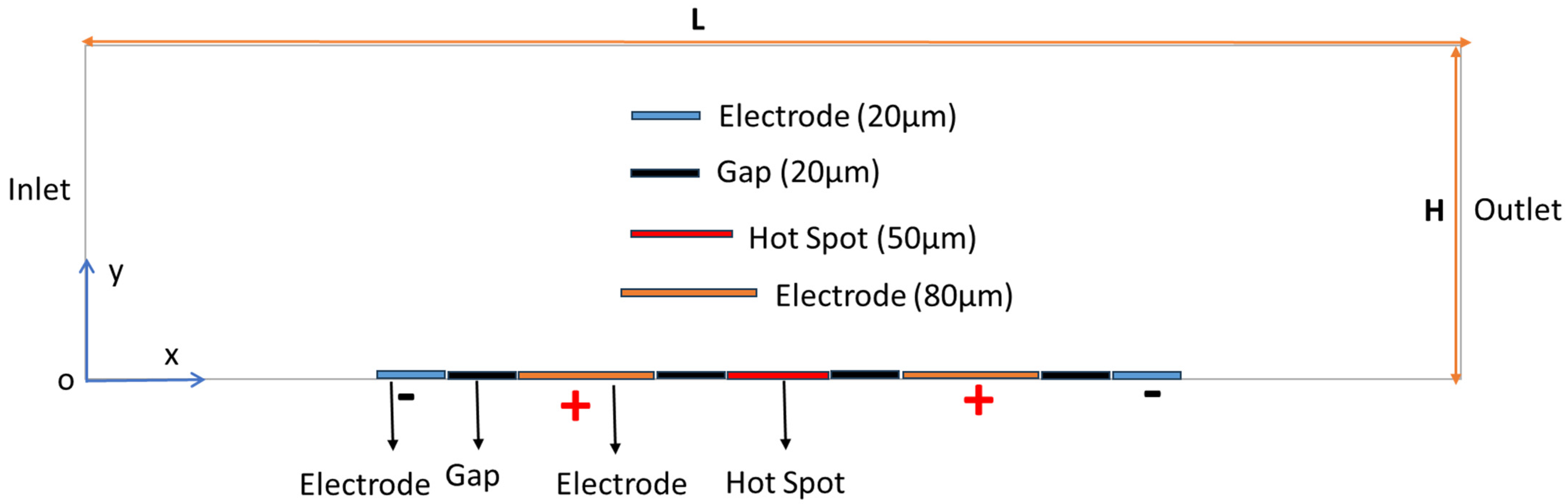
2.2. AC Electrothermal Schematic
2.3. Boundary Conditions
2.4. Mesh
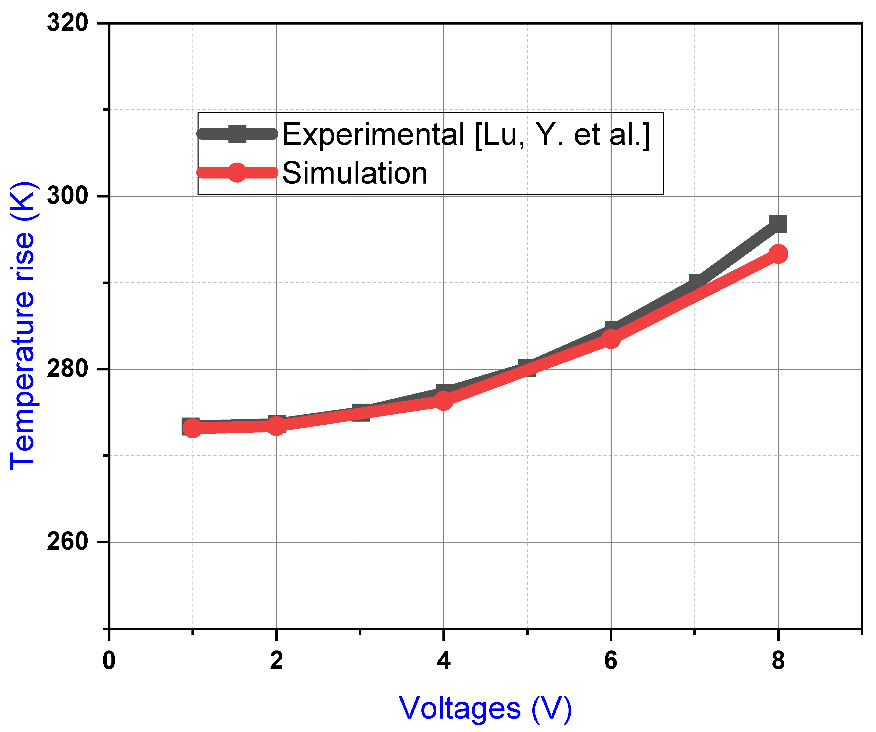
2.5. Validation
3. Simulations and Results
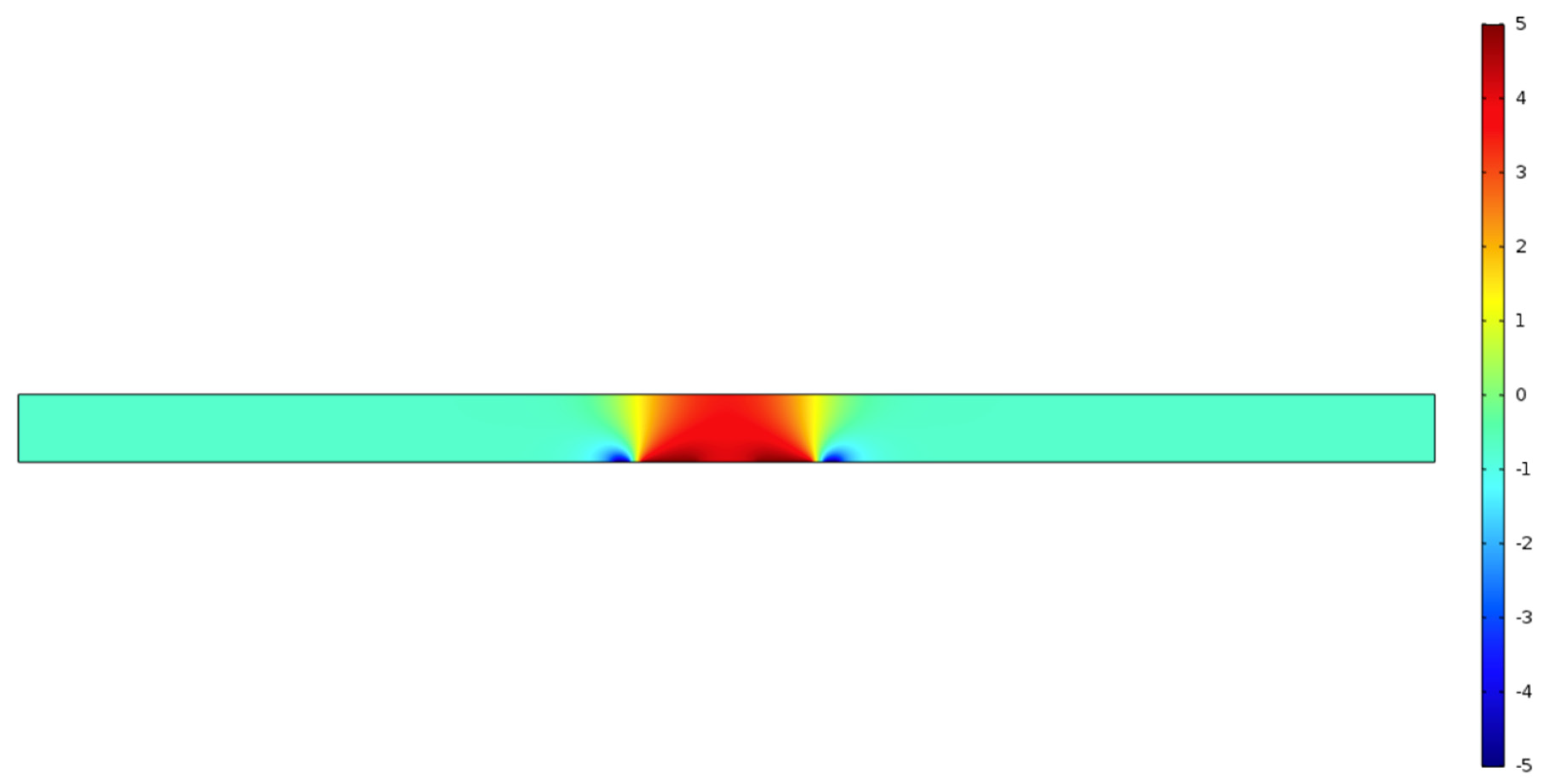
3.1. The Electrical Potential
3.2. Electrode Size
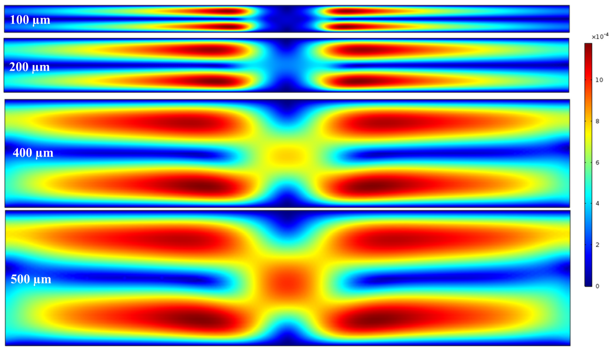
3.3. Fluid Velocities
3.4. Channel Dimensions
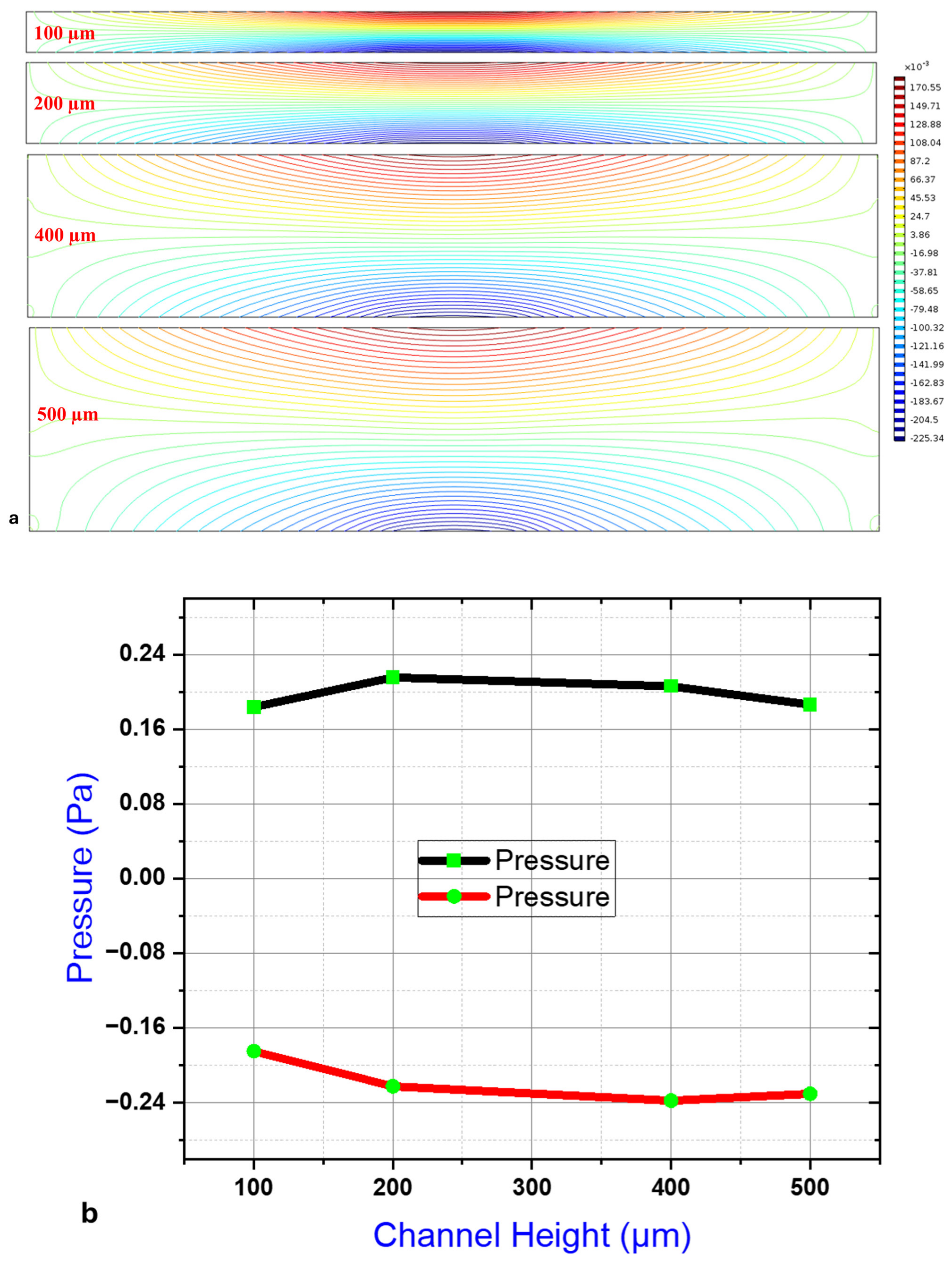
3.5. Pressure Gradients
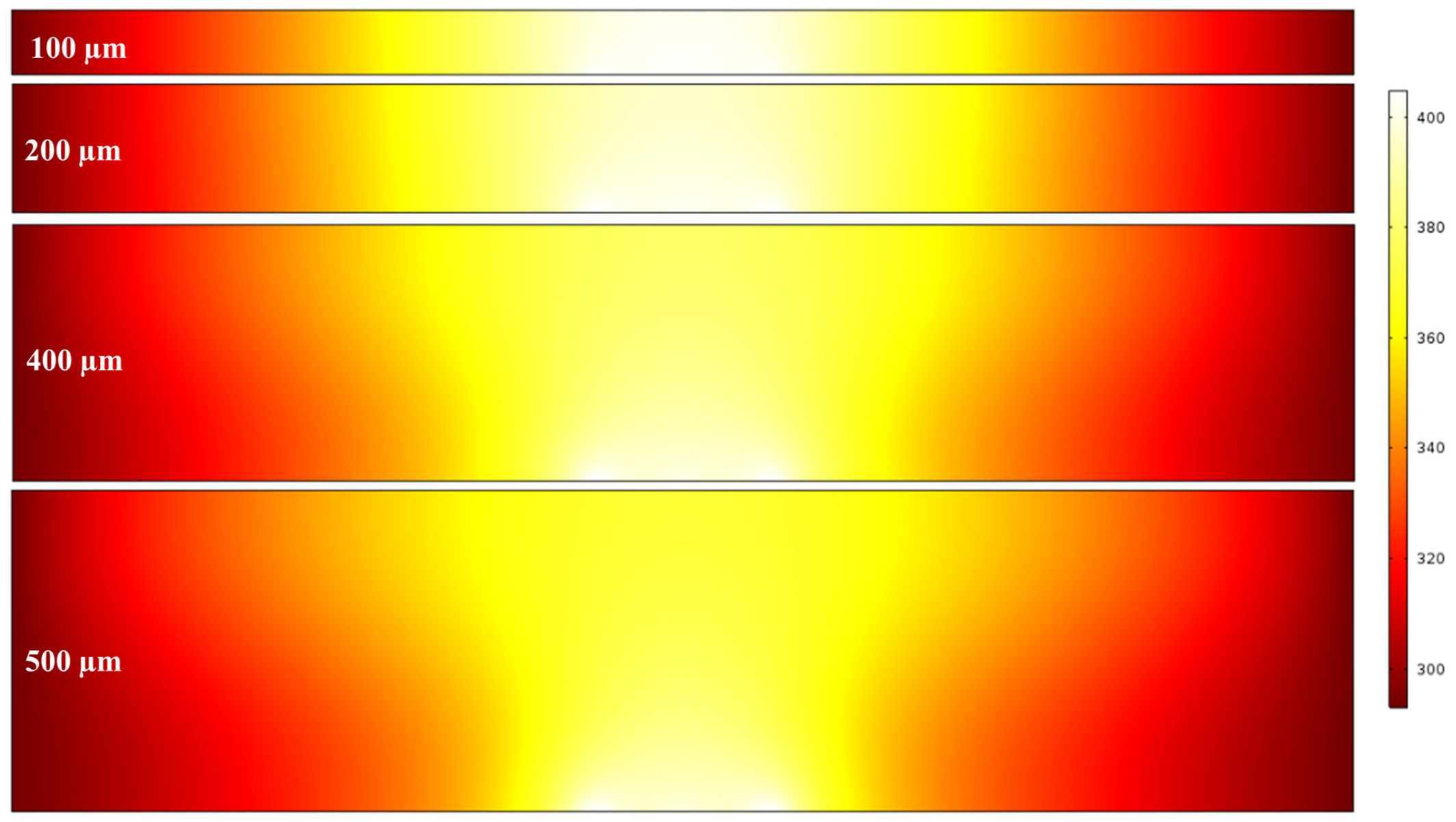
3.6. Temperature
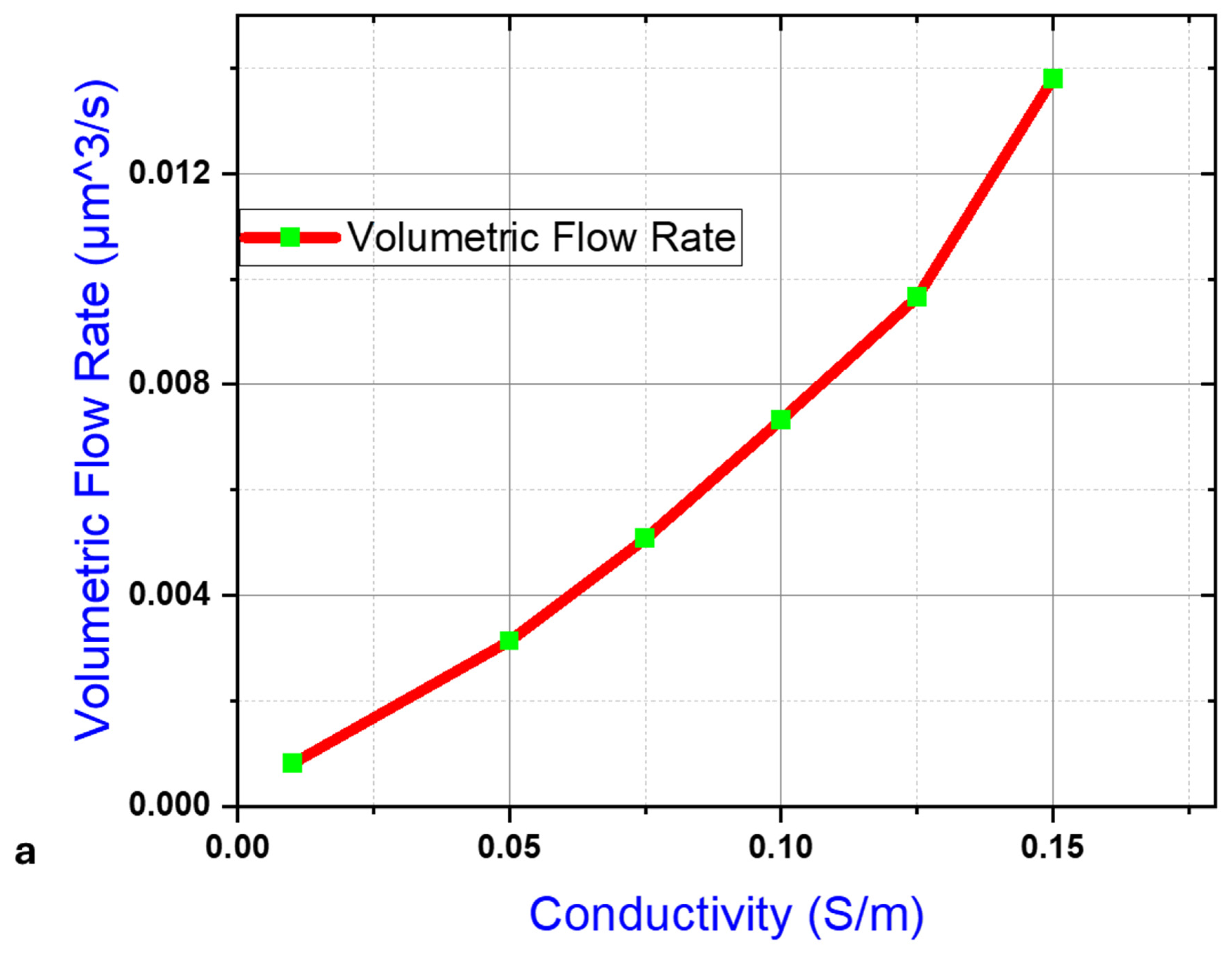
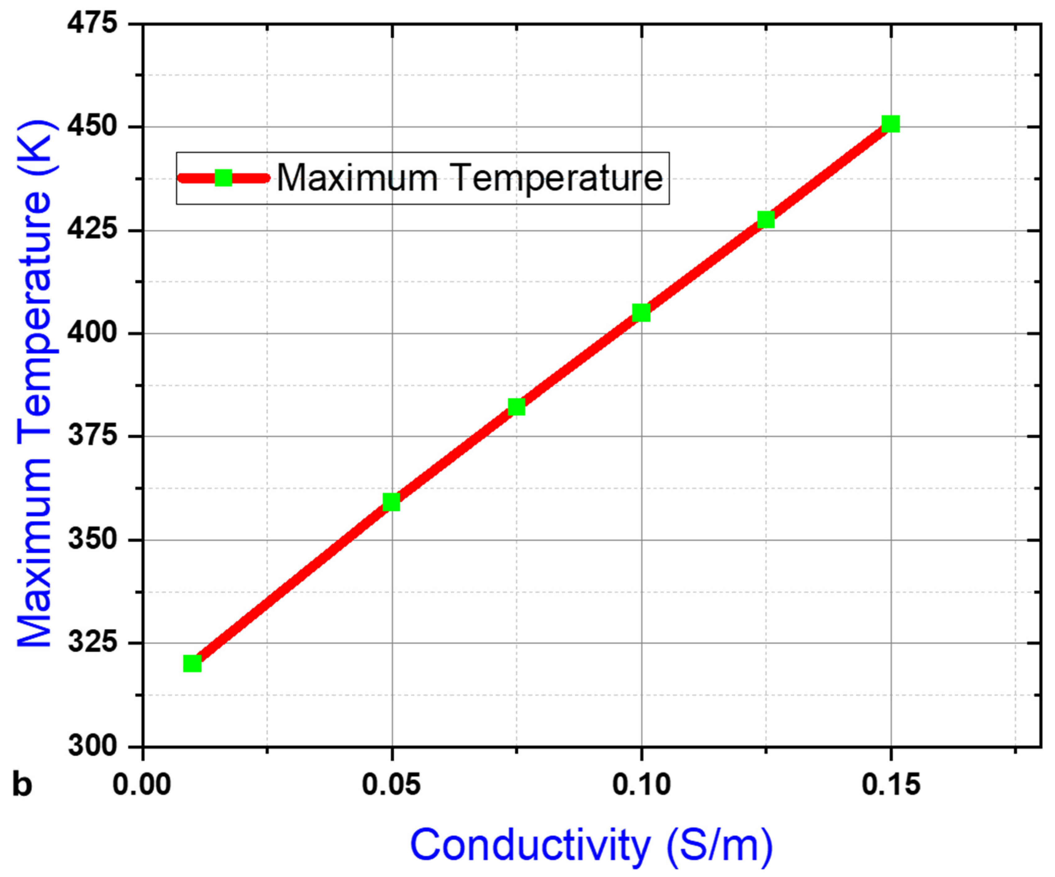
3.7. Fluid Conductivity
3.8. Voltage and Flow Rate
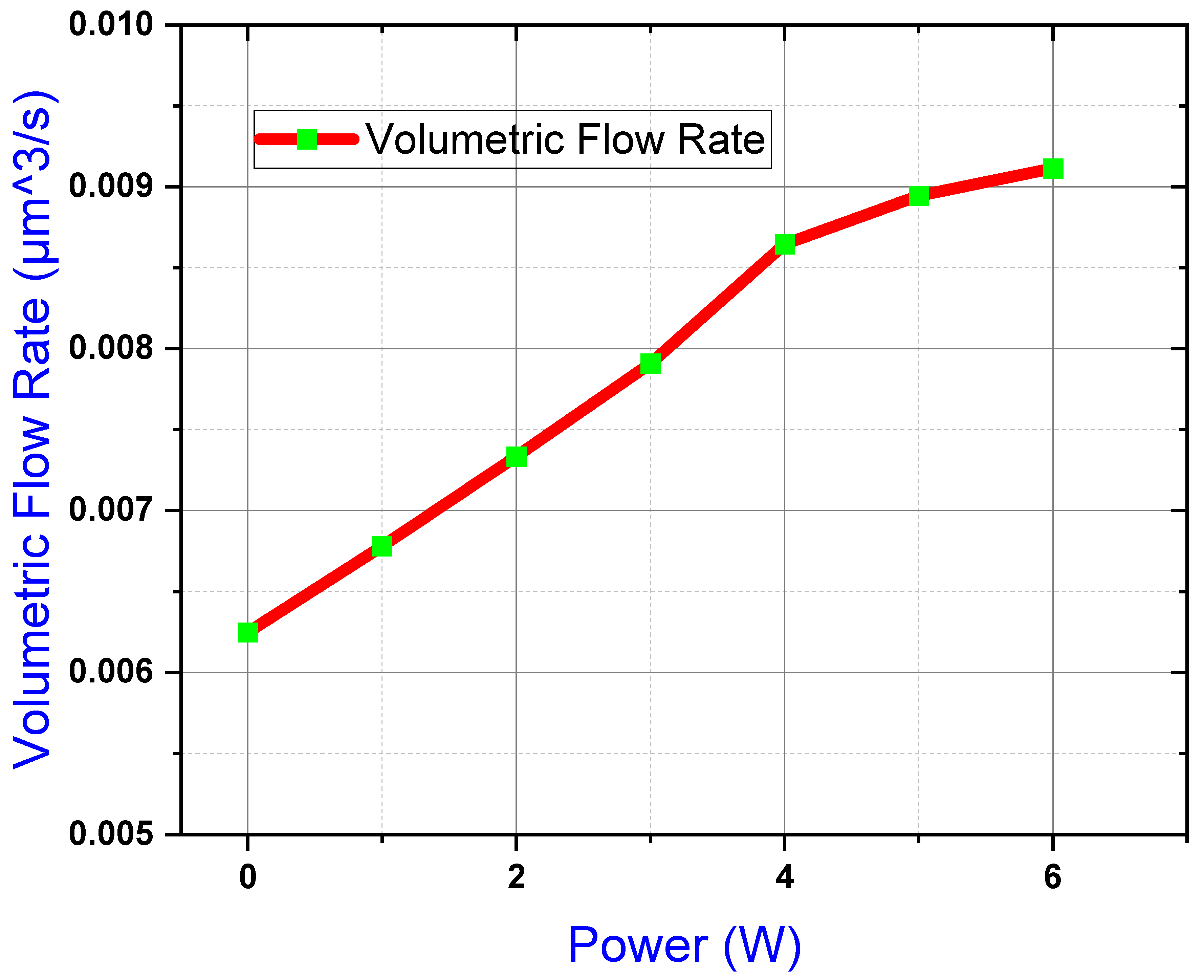
3.9. Power and Flow Rate
4. Discussion
4.1. Results Discussion
4.2. Potential Applications, Limitations, and Future Work Toward Validation
4.3. On Overcoming Modeling Limitations
5. Conclusions
Author Contributions
Funding
Institutional Review Board Statement
Informed Consent Statement
Data Availability Statement
Acknowledgments
Conflicts of Interest
References
- Hossan, M.R.; Dutta, D.; Islam, N.; Dutta, P. Electric field driven pumping in microfluidic device. Electrophoresis 2018, 39, 702–731. [Google Scholar] [CrossRef]
- Dutta, D.; Palmer, X.; Lim, J.Y.; Chandra, S. Simulation on the Separation of Breast Cancer Cells within a Dual-Patterned End Microfluidic Device. Fluids 2024, 9, 123. [Google Scholar] [CrossRef]
- Dutta, D.; Smith, K.; Palmer, X. Long-Range ACEO Phenomena in Microfluidic Channel. Surfaces 2023, 6, 145–163. [Google Scholar] [CrossRef]
- Das, D.; Yan, Z.; Menon, N.V.; Kang, Y.; Chan, V.; Yang, C. Continuous detection of trace level concentration of oil droplets in water using microfluidic AC electroosmosis (ACEO). Rsc Adv. 2015, 5, 70197–70203. [Google Scholar] [CrossRef]
- Bazant, M.Z.; Urbanski, J.P.; Levitan, J.A.; Subramanian, K.; Kilic, M.S.; Jones, A.; Thorsen, T. Electrolyte dependence of AC electro-osmosis. Micro Total Anal. Syst. 2007, 1, 285–287. [Google Scholar]
- Dutta, D.; Russell, C.; Kim, J.; Chandra, S. Differential mobility of breast cancer cells and normal breast epithelial cells under DC electrophoresis and electroosmosis. Anticancer. Res. 2018, 38, 5733–5738. [Google Scholar] [CrossRef] [PubMed]
- Ghandchi, M.; Vafaie, R.H. AC electrothermal actuation mechanism for on-chip mixing of high ionic strength fluids. Microsyst. Technol. 2017, 23, 1495–1507. [Google Scholar] [CrossRef]
- Franke, T.A.; Wixforth, A. Microfluidics for miniaturized laboratories on a chip. ChemPhysChem 2008, 9, 2140–2156. [Google Scholar] [CrossRef]
- Sharma, B.; Sharma, A. Microfluidics: Recent advances toward lab-on-chip applications in bioanalysis. Adv. Eng. Mater. 2022, 24, 2100738. [Google Scholar] [CrossRef]
- Han, K.N.; Li, C.A.; Seong, G.H. Microfluidic chips for immunoassays. Annu. Rev. Anal. Chem. 2013, 6, 119–141. [Google Scholar] [CrossRef]
- Burdallo, I.; Jimenez-Jorquera, C.; Fernández-Sánchez, C.; Baldi, A. Integration of microelectronic chips in microfluidic systems on printed circuit board. J. Micromech. Microeng. 2012, 22, 105022. [Google Scholar] [CrossRef]
- Yoon, Y.; Kwon, Y.; Park, H.; Lee, S.; Park, C.; Lee, T. Recent Progress in Rapid Biosensor Fabrication Methods: Focus on Electrical Potential Application. BioChip J. 2024, 18, 1–21. [Google Scholar] [CrossRef]
- Yuan, Q.; Wu, J. Thermally biased AC electrokinetic pumping effect for lab-on-a-chip based delivery of biofluids. Biomed. Microdevices 2013, 15, 125–133. [Google Scholar] [CrossRef] [PubMed]
- Xiong, H.; Zhu, C.; Dai, C.; Ye, X.; Li, Y.; Li, P.; Yang, S.; Ashraf, G.; Wei, D.; Chen, H.; et al. An Alternating Current Electroosmotic Flow-Based Ultrasensitive Electrochemiluminescence Microfluidic System for Ultrafast Monitoring, Detection of Proteins/miRNAs in Unprocessed Samples. Adv. Sci. 2024, 11, 2307840. [Google Scholar] [CrossRef]
- Kumar, A.; Manna, N.K.; Sarkar, S.; Biswas, N. Enhancing mixing efficiency of a circular electroosmotic micromixer with cross-reciprocal electrodes. Phys. Fluids 2024, 36, 083626. [Google Scholar] [CrossRef]
- Zhou, J.; Tao, Y.; Liu, W.; Sun, T.; Wu, F.; Shi, C.; Ren, Y. A portable and integrated traveling-wave electroosmosis microfluidic pumping system driven by triboelectric nanogenerator. Nano Energy 2024, 127, 109736. [Google Scholar] [CrossRef]
- Salari, A.; Navi, M.; Lijnse, T.; Dalton, C. AC electrothermal effect in microfluidics: A review. Micromachines 2019, 10, 762. [Google Scholar] [CrossRef]
- Hong, F.J.; Cao, J.; Cheng, P. A parametric study of AC electrothermal flow in microchannels with asymmetrical interdigitated electrodes. Int. Commun. Heat Mass Transf. 2011, 38, 275–279. [Google Scholar] [CrossRef]
- Liu, Z.P.; Speetjens, M.F.M.; Frijns, A.J.H.; Van Steenhoven, A.A. Heat-transfer enhancement in AC electro-osmotic micro-flows. J. Phys. Conf. Ser. 2012, 395, 012094. [Google Scholar] [CrossRef]
- Ren, Q. Investigation of pumping mechanism for non-Newtonian blood flow with AC electrothermal forces in a microchannel by hybrid boundary element method and immersed boundary-lattice Boltzmann method. Electrophoresis 2018, 39, 1329–1338. [Google Scholar] [CrossRef]
- Loire, S.; Kauffmann, P.; Mezić, I.; Meinhart, C.D. A theoretical and experimental study of ac electrothermal flows. J. Phys. D: Appl. Phys. 2012, 45, 185301. [Google Scholar] [CrossRef]
- Sasaki, N.; Kitamori, T.; Kim, H.B. Fluid mixing using AC electrothermal flow on meandering electrodes in a microchannel. Electrophoresis 2012, 33, 2668–2673. [Google Scholar] [CrossRef] [PubMed]
- Lu, Y.; Ren, Q.; Liu, T.; Leung, S.L.; Gau, V.; Liao, J.C.; Chan, C.L.; Wong, P.K. Long-range electrothermal fluid motion in microfluidic systems. Int. J. Heat Mass Transf. 2016, 98, 341–349. [Google Scholar] [CrossRef]
- Edayan, J.M.; Gallemit, A.J.; Sacala, N.E.; Palmer, X.L.; Potter, L.; Rarugal, J.P.; Velasco, L.C. Integration Technologies in Laboratory Information Systems: A Systematic Review. Inform. Med. Unlocked 2024, 50, 101566. [Google Scholar] [CrossRef]
- Henning, A.K.; Fitch, J.S.; Harris, J.M.; Dehan, E.B.; Cozad, B.A.; Christel, L.; Fathi, Y.; Hopkins, D.A.; Lilly, L.J.; McCulley, W.; et al. Microfluidic MEMS for semiconductor processing. IEEE Trans. Compon. Packag. Manuf. Technol. Part B 1998, 21, 329–337. [Google Scholar] [CrossRef]
- Koklu, A.; Tansel, O.; Oksuzoglu, H.; Sabuncu, A.C. Electrothermal flow on electrodes arrays at physiological conductivities. Iet Nanobiotechnol. 2016, 10, 54–61. [Google Scholar] [CrossRef] [PubMed]
- Wu, J.; Lian, M.; Yang, K. Micropumping of biofluids by alternating current electrothermal effects. Appl. Phys. Lett. 2007, 90, 101566. [Google Scholar] [CrossRef]
- Williams, S.J. Enhanced electrothermal pumping with thin film resistive heaters. Electrophoresis 2013, 34, 1400–1408. [Google Scholar] [CrossRef] [PubMed]
- Zhang, R.; Dalton, C.; Jullien, G.A. Two-phase AC electrothermal fluidic pumping in a coplanar asymmetric electrode array. Microfluid. Nanofluidics 2011, 10, 521–529. [Google Scholar] [CrossRef]
- Ren, Q.; Wang, Y.; Lin, X.; Chan, C.L. AC electrokinetic induced non-Newtonian electrothermal blood flow in 3D microfluidic biosensor with ring electrodes for point-of-care diagnostics. J. Appl. Phys. 2019, 126, 084501. [Google Scholar] [CrossRef]
- Kunti, G.; Bhattacharya, A.; Chakraborty, S. Analysis of micromixing of non-Newtonian fluids driven by alternating current electrothermal flow. J. Non-Newton. Fluid Mech. 2017, 247, 123–131. [Google Scholar] [CrossRef]
- Verpoorte, E.; De Rooij, N.F. Microfluidics meets MEMS. Proc. IEEE 2003, 91, 930–953. [Google Scholar] [CrossRef]
- Du, B.; Hudgins, J.L.; Santi, E.; Bryant, A.T.; Palmer, P.R.; Mantooth, H.A. Transient electrothermal simulation of power semiconductor devices. IEEE Trans. Power Electron. 2009, 25, 237–248. [Google Scholar]
- Kunti, G.; Dhar, J.; Chakraborty, S.; Bhattacharya, A. Alternating Current Electrothermal Flow for Cooling of Localized Hot Spots in Microelectronic Devices. IEEE Trans. Compon. Packag. Manuf. Technol. 2020, 10, 1020–1027. [Google Scholar] [CrossRef]
- Ghaisas, G.; Krishnan, S. Thermal influence coefficients-based electrothermal modeling approach for power electronics. IEEE Trans. Compon. Packag. Manuf. Technol. 2021, 11, 1187–1196. [Google Scholar] [CrossRef]
- Sanz-Alcaine, J.M.; Sebastián, E.; Perez-Cebolla, F.J.; Arruti, A.; Bernal-Ruiz, C.; Aizpuru, I. Estimation of Semiconductor Power Losses Through Automatic Thermal Modeling. IEEE Trans. Power Electron. 2024, 39, 11086–11098. [Google Scholar] [CrossRef]
- Williams, S.J.; Green, N.G. Electrothermal pumping with interdigitated electrodes and resistive heaters. Electrophoresis 2015, 36, 1681–1689. [Google Scholar] [CrossRef]


| Parameter | Value | Description |
|---|---|---|
| Σ | 0.1 [S/m] | Conductivity of the ionic solution |
| 80.8 × 8.85 × 10−12 [F/m] | Relative permittivity | |
| V0 | 5 [V] | Maximum value of the applied voltage |
| 1000 [kg/m3] | Water density | |
| T0 | 293.15 [K] | Room temperature |
| L | 2090 [µm] | Channel length |
| H | 100 [µm] | Channel height |
| 9.81 [m/s2] | Acceleration due to gravity | |
| µ | 0.001 [Pa·s] | Dynamic viscosity of the water |
| cc | 4184 [J/kg °C] | Specific heat capacity of water |
| kk | 0.6 [W/(m·K)] | Thermal conductivity of water |
Disclaimer/Publisher’s Note: The statements, opinions and data contained in all publications are solely those of the individual author(s) and contributor(s) and not of MDPI and/or the editor(s). MDPI and/or the editor(s) disclaim responsibility for any injury to people or property resulting from any ideas, methods, instructions or products referred to in the content. |
© 2025 by the authors. Licensee MDPI, Basel, Switzerland. This article is an open access article distributed under the terms and conditions of the Creative Commons Attribution (CC BY) license (https://creativecommons.org/licenses/by/4.0/).
Share and Cite
Dutta, D.; Mei, L.; Palmer, X.; Ziemke, M. Energy-Efficient AC Electrothermal Microfluidic Pumping via Localized External Heating. Appl. Sci. 2025, 15, 7369. https://doi.org/10.3390/app15137369
Dutta D, Mei L, Palmer X, Ziemke M. Energy-Efficient AC Electrothermal Microfluidic Pumping via Localized External Heating. Applied Sciences. 2025; 15(13):7369. https://doi.org/10.3390/app15137369
Chicago/Turabian StyleDutta, Diganta, Lanju Mei, Xavier Palmer, and Matthew Ziemke. 2025. "Energy-Efficient AC Electrothermal Microfluidic Pumping via Localized External Heating" Applied Sciences 15, no. 13: 7369. https://doi.org/10.3390/app15137369
APA StyleDutta, D., Mei, L., Palmer, X., & Ziemke, M. (2025). Energy-Efficient AC Electrothermal Microfluidic Pumping via Localized External Heating. Applied Sciences, 15(13), 7369. https://doi.org/10.3390/app15137369