Abstract
Road traffic accidents remain a critical public health concern worldwide, with Poland consistently experiencing high fatality rates—52 deaths per million inhabitants in 2023, compared to the EU average of 46. To investigate the underlying factors contributing to these accidents, we developed a multifactorial dataset integrating 250,000 accident records from 2015 to 2023 with spatially interpolated weather data and sociodemographic indicators. We employed Kriging interpolation to convert point-based weather station data into continuous surfaces, enabling the attribution of location-specific weather conditions to each accident. Following comprehensive preprocessing and spatial analysis, we generated visualizations—including heatmaps and choropleth maps—that revealed distinct regional patterns at the county level. Our preliminary findings suggest that accident occurrence and severity are driven by different underlying factors: while temperature and vehicle counts strongly correlate with total accident numbers, humidity, precipitation, and road infrastructure quality show stronger associations with fatal outcomes. This integrated dataset provides a robust foundation for Bayesian and time-series modeling, supporting the development of evidence-based road safety strategies.
1. Introduction
Road traffic accidents (RTAs) remain a substantial threat to public health and economic stability worldwide. According to the World Health Organization (WHO), approximately 1.19 million people lose their lives each year as a result of RTAs [1]. While Poland has witnessed a significant decline in accident rates and fatalities in recent years, its figures remain elevated relative to many other European Union member states [2]. Their adverse outcomes have significant implications not only for healthcare systems and emergency response mechanisms but also for broader social and economic structures. The multifactorial nature of road accidents necessitates an investigation that goes beyond isolated incident reports to consider a confluence of environmental, infrastructural, and sociodemographic factors.
Effective mitigation of the consequences of RTAs requires precise identification and thorough interpretation of their causes. While extensive scientific research has been conducted on this topic, the intricate and multifaceted nature of RTAs continues to make isolating key contributing factors and accurately assessing their influence a significant challenge. Multiple studies highlight that RTAs are influenced by a range of variables spanning weather conditions, road infrastructure, vehicle condition, and driver behavior [3]. For instance, low friction on snow- and ice-covered roads significantly increases the likelihood of collisions, underscoring the importance of road maintenance in adverse conditions [4]. Temperature similarly plays a crucial role and has been associated with increasing the risk of crashes [5], especially due to the fact that high temperatures impair driver concentration or encourage riskier behavior [6]. Heatwaves increase this risk even more [7]. Conversely, subzero temperatures do not necessarily pose a direct threat unless they result in ice formation and snow accumulation, which dramatically raises the probability of incidents, but lowers the number of fatal cases [4]. It should be noted that many of those results are related to the location of research; for example, Andersson et al. found no direct correlation between rising temperature and traffic safety in Sweden [8], yet Basagana et al. found an almost linear correlation in that aspect in Spain [9]. Beyond weather, sociodemographic factors such as population density and vehicle ownership, which increase traffic volume, also shape accident occurrence [10], while infrastructural aspects—ranging from road geometry to surface quality—exert an additional influence. Together, these findings underscore that no single variable fully accounts for the complexity of RTA dynamics, reinforcing the need for integrated models capable of capturing diverse environmental and human-related factors.
While traditional research has focused primarily on engineering, behavioral, and regulatory factors, increasing attention variables (apart from sociodemographic factors), has been directed toward broader socioeconomic. Among these, tourism and fuel prices have emerged as influential factors associated with road safety outcomes. Tourism can alter traffic volume, composition, and patterns, introducing unfamiliar drivers into local systems. Likewise, fluctuations in fuel prices can influence travel behavior, vehicle usage, and traffic exposure. Socioeconomic factors—such as tourism and fuel prices—and their relationship with road traffic accidents have been widely analyzed in the literature. In particular, the link between tourism and road traffic accidents has been examined across various contexts. Burke and Nishitateno [11] exploited significant international variation in gasoline pump prices to investigate the impact of fuel costs on road traffic fatalities. Utilizing data from 144 countries spanning the period 1991–2010, their study provided the first international estimates of the gasoline price elasticity of road fatalities. Their findings suggest that a 10% increase in gasoline pump prices is associated with a 3–6% reduction in road fatalities. The authors estimate that approximately 35,000 road deaths annually could be prevented through the elimination of global fuel subsidies. Psarras et al. [12] analyzed data from 51 Greek NUTS-3 regions over the period 2000–2017 to examine the role of tourism in road accident incidence. Their study evaluated the influence of tourism alongside economic, demographic, meteorological, and exposure-related variables. Their results indicate that tourism significantly affects road accident rates in Greece, with foreign tourists playing a particularly influential role. Bellos et al. [13] also investigated the relationship between tourism and road traffic incidents in Greece. Using police-reported crash data from 2011 to 2015, their study incorporated variables such as driver nationality, travel season, travel purpose, and geographic region. Negative binomial regression models were employed to analyze the data, revealing that tourists are statistically more likely to be involved in road crashes compared to local drivers. Grabowski and Morrisey [14] examined the potential for increased fuel taxes to reduce traffic fatalities. Their study posits that higher fuel taxes lead to increased gasoline prices, which in turn reduce gasoline consumption and, consequently, traffic fatalities. Castillo-Manzano et al. [15] explored the impact of tourism on road safety in Spain—a particularly relevant case given the country’s status as the world’s second most-visited destination over several consecutive years. Focusing on Spanish NUTS-3 regions, the authors found that foreign drivers were associated with higher traffic accident rates, highlighting the need to incorporate tourism-related factors into road safety policy planning. Naqvi et al. [16] assessed the relationship between fuel prices and road traffic accident frequency through the lens of travel behavior adjustments. Weekly fuel price data from 2005 to 2015 were analyzed using the Prais–Winsten autoregressive model of the first order (AR1) and the Box–Jenkins seasonal autoregressive integrated moving average (SARIMA) models. The study concluded that a 1% increase in fuel price results in a 0.4% decrease in fatal road traffic accidents. Recently, Quest and Will [17] focused on the statistical modeling and prediction of road traffic accident patterns. Employing a combination of traditional statistical techniques—such as Poisson and negative binomial regression—and modern machine learning methods, including random forests and deep learning algorithms, their study aimed to enhance the accuracy of accident hotspot detection. Geospatial analysis and time-series forecasting were also utilized to assess accident frequency and severity across time and space.
A wide range of analytical methods have been employed to study the occurrence of RTAs, ranging from traditional statistical approaches to advanced machine learning techniques [3]. Classical methods such as negative binomial models [18], time-series analysis [6,19], regression analysis [20], and Poisson regression models [10] have long been used to identify relationships between accident frequency and contributing factors. While these methods offer interpretability and robustness, they often struggle to capture the complex, nonlinear interactions present in real-world accident data. More recently, data-driven techniques, including artificial neural networks (ANNs), support vector machines (SVMs), and random forests, have gained traction due to their ability to model intricate patterns and improve predictive accuracy [21]. Among these, deep learning models, particularly recurrent and convolutional neural networks, represent a novel approach with promising results in time-series and spatial accident prediction. Hybrid models that integrate statistical and machine learning techniques have also been proposed to leverage the strengths of both paradigms [22]. Despite these advancements, challenges remain, particularly regarding data quality, feature selection, and model interpretability, highlighting the need for continued methodological refinement in RTA analysis.
Although many studies focus on identifying accident risk factors, a growing number explicitly aim to forecast the future number of accidents. For instance, some works adopt ARIMA or exponential smoothing to predict monthly or daily crash frequencies [6,19], whereas others leverage advanced data-driven methods—such as neural networks or hybrid models—to capture nonlinear trends in accident occurrence [23]. These forecasting approaches provide crucial insights for policy planning and resource allocation, yet they remain susceptible to the inherent volatility of traffic systems, underscoring the importance of ongoing research to enhance both accuracy and interpretability.
Effective analysis of the impact of weather conditions on road accidents requires accurate information about the weather at the time of each recorded incident. However, historical data are typically collected only from a sparse network of meteorological stations, restricting direct observational capabilities. To overcome this issue, a range of spatial interpolation approaches has been explored in meteorology and hydrology, specifically designed to generate spatially continuous fields from limited point observations. Several studies have investigated simpler interpolation approaches such as Thiessen polygons, inverse distance weighting (IDW), and areal averages. Dirks et al. concluded that IDW offered a balance of simplicity and accuracy, but only when station density was relatively high [24]. Similarly, Stow et al. underscored the significance of station density and local variability, arguing that precipitation is a rapidly changing, localized phenomenon [25]. Berne et al. further highlighted the importance of high temporal resolution—often beyond the capacity of operational radars—particularly in urban areas [26].
Kriging has emerged as one of the most robust geostatistical methods for interpolating meteorological variables, thanks to its ability to exploit the spatial autocorrelation of observations [27]. In its simplest (ordinary) form, kriging estimates unknown values by modeling the variogram of the variable of interest [28]. Given the complexity of real-world environments, many studies have expanded this method by combining it with other data-driven or physical modeling approaches to refine spatial estimates of meteorological variables. Multivariate kriging methods, such as kriging with external drift (KED) or co-kriging, incorporate auxiliary variables like digital elevation models [29,30], land cover [31], or solar irradiance [32] to correct for local climate effects and enhance predictive accuracy. Researchers also investigate temporal kriging approaches for filling gaps in time-series data [33]. The primary advantages of kriging lie in its ability to quantify estimation uncertainty and adapt to localized spatial structures, making it especially suitable for capturing fine-scale variations. However, it can be computationally demanding, and despite its robustness, its performance is also closely tied to the quality and density of the station network [24].
In light of these challenges, the present study aims to construct a comprehensive dataset that amalgamates detailed accident records with corresponding weather data and sociodemographic indicators, offering a promising avenue for investigation, facilitating the identification of statistically significant relationships among these variables and enabling the application of advanced statistical methodologies to rigorously quantify uncertainty and capture regional heterogeneity. By assembling and visualizing these interconnected data streams, this study seeks to illuminate potential links between environmental conditions and accident dynamics. The resulting dataset is intended to serve as a foundational resource for subsequent analyses, including time-series forecasting and causal inference studies, ultimately contributing to a more nuanced understanding of road safety issues in Poland, and is prepared to be utilized in Bayesian modeling aimed at road traffic accident prediction.
This introductory section establishes the rationale for the study, providing a foundation for the subsequent analysis of the factors influencing RTAs in Poland and presenting a comprehensive review of the relevant literature, offering deeper insight into the complex relationships between accident frequency, weather conditions, and sociodemographic factors. The following section details the data collection process, as well as the preprocessing and visualization techniques employed to ensure the accuracy and clarity of the dataset. Section 3 delves into the results, analyzing the key findings derived from the processed data. Finally, Section 4 summarizes this study’s conclusions, highlighting its implications and potential avenues for future research.
2. Materials and Methods
2.1. Data Sources
The data collection phase of this study integrated three distinct yet complementary datasets from authoritative national sources involving traffic accident records, meteorological data, and socioeconomic data.
The primary source for traffic accident records was the Accident and Collision Recording System (SEWIK), a national database supervised by the Traffic Bureau of the National Police Headquarters [34]. SEWIK provides comprehensive information on each reported incident, including the date, time, and geographic location, as well as details on accident type, severity, casualties, and property damage. Part of this database is publicly available through the Polish Road Safety Observatory (POBRD), ensuring transparency and ease of data retrieval [35]. In addition, SEWIK’s data were also gathered from a non-commercial service sewik.pl [36]. While this source contains supplementary information not readily available in POBRD, its lack of official status raises concerns regarding data accuracy and completeness. Therefore, both sources were analyzed to identify potential discrepancies, ensuring the highest possible data reliability.
The meteorological data utilized in this study were sourced from the Institute of Meteorology and Water Management (IMGW) [37], Poland’s principal source of weather observations, operating under the Ministry of Infrastructure [38]. IMGW maintains an extensive network of meteorological and hydrological stations across the country, as shown in Figure 1, systematically collecting high-resolution data [39]. The publicly available historical records include key atmospheric parameters such as temperature, precipitation, and relative humidity. Although IMGW’s dataset provides sufficient temporal resolution, the uneven spatial distribution of its stations introduces challenges that might affect the precision of weather interpolation between monitoring locations.
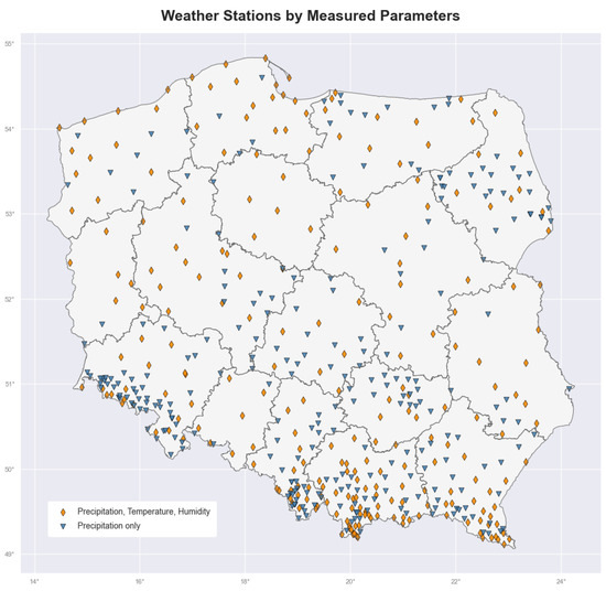
Figure 1.
Geographic distribution of IMGW’s weather stations across Poland active during the study period. Stations are categorized by their measurement capabilities: those measuring precipitation, temperature, and humidity, and those measuring precipitation only. The network shows broader spatial coverage for precipitation measurements, with a particularly dense concentration of both station types in the south, mountainous regions. Northern and central regions display a more dispersed pattern with relatively fewer stations, while maintaining a fairly balanced distribution between full-parameter and precipitation-only stations throughout the country.
Socioeconomic data were obtained from the Local Data Bank of Statistics Poland (GUS), the nation’s primary source of official statistics [40]. GUS provides detailed insights into key indicators such as population density, vehicle registrations, and road network coverage across Poland’s hierarchical administrative divisions (municipalities, counties, voivodeships) and at the national aggregate level. These variables serve as proxies for regional traffic exposure and infrastructural development. By integrating these factors, the study aims to assess the role of regional disparities in shaping road accident dynamics, ensuring a more holistic perspective on the complex interplay between environmental, infrastructural, and human-related determinants.
To enhance the accuracy of meteorological data interpolation, Poland’s elevation information was sourced from the Digital Elevation Model (DEM) acquired from the Geographic Information System of the Commission (GISCO) [41]. These data played a meaningful role in refining the spatial distribution of weather parameters, allowing for a more precise representation of local conditions.
Additionally, information on the administrative boundaries of Poland’s voivodeships and counties was obtained from the National Register of Boundaries (PRG) [42]. These boundary datasets were subsequently employed to help estimate average weather conditions within each administrative unit and to facilitate data visualization.
2.2. Meteorological Data Interpolation
Historical weather data are available solely at the locations of meteorological stations, whose network is both unevenly distributed across the country and sparse, particularly in relation to the localized county-level context of the dataset (Figure 1). This uneven distribution of meteorological stations creates challenges in directly linking weather conditions to specific accident locations, especially in areas where stations are distant or lacking. The data gaps posed by the spatial limitations of this network could lead to inaccurate or incomplete weather information for certain regions.
Before performing the analysis, we split the meteorological stations into two categories: those that exclusively record precipitation data and those that, in addition to precipitation, offer temperature and humidity measurements. The number of stations collecting precipitation data is more than twice that of stations providing the additional meteorological parameters. While this higher station density improves spatial coverage for precipitation measurements, accurately estimating precipitation conditions remains particularly challenging due to its variability and highly localized nature [25]. Unlike temperature and humidity, which exhibit smoother spatial patterns, precipitation can be influenced by small-scale atmospheric processes, making interpolation and extrapolation more complex.
We used a histogram to examine the distance between each incident location and the nearest meteorological station from the IMGW network that was operational at the time of the incident, calculated based on their geographic coordinates (Figure 2). The results reveal that the majority of accidents occurred within 12 km of a station providing precipitation measurements and within 16 km of a station recording temperature and humidity data. These proximities suggest that, for a significant portion of cases, the available meteorological observations offer a reasonable approximation of local weather conditions. However, a substantial number of accidents were recorded at much greater distances—exceeding 40 km for precipitation data and 60 km for temperature and humidity measurements. This spatial disparity, especially for precipitation, increases the likelihood of notable inaccuracies in the estimated weather conditions at accident sites.
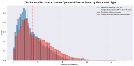
Figure 2.
Distribution of distances between incident locations and the nearest weather stations operational at the time, categorized by measurement type. The dotted lines indicate the median distances for stations measuring relevant parameters. Precipitation measurements (blue) show a median distance of 11.9 km with density peaking at approximately 10 km, while temperature and humidity measurements (red) exhibit a broader distribution with a median distance of 15.9 km, reflecting the lower number of stations measuring these parameters. Both distributions are right-skewed, with most incidents occurring within 20 km of a weather station, though measurements at longer distances (>20 km) are more prevalent for temperature and humidity than for precipitation.
To address the challenge of accurately estimating weather conditions, we employed kriging to interpolate temperature, humidity, and precipitation across Poland. Kriging is a geostatistical interpolation method that provides the best linear unbiased predictions for unsampled locations by leveraging the spatial autocorrelation present in observed data. Its strength lies in effectively incorporating spatial dependencies among observations, making it particularly suitable for modeling continuously varying phenomena like temperature.
Utilizing the geolocation data of weather stations provided by IMGW, we were able to generate a continuous data surface from discrete measurements. By incorporating data from multiple stations, kriging reduces the impact of large observation gaps, particularly for precipitation, where localized variability can be significant. To enhance interpolation accuracy, we incorporated elevation data as a drift term in the kriging process, which proved especially valuable for mountainous regions where topography significantly influences weather patterns. This approach allowed us to overcome the limitations of station density variability, ensuring that even regions with sparse observational coverage were accurately represented.
Together, the interpolated data provided a comprehensive representation of weather conditions across Poland at any given time, enabling a detailed analysis of how varying meteorological factors influence road traffic incidents.
2.3. Dataset
The dataset consists of three tables. The first table contains accident data from SEWIK supplemented with interpolated weather conditions and socioeconomic indicators. The second table presents daily weather data aggregated at the county level covering the same period. The third table includes yearly socioeconomic indicators from GUS, organized hierarchically across multiple administrative levels (counties, voivodeships, and national aggregates).
Variables marked with • in Table 1 originate from the SEWIK database. Columns providing precise incident location information and site-specific conditions were selected. While additional participant details such as gender, age, and driving experience are contained in SEWIK, only the information on whether any participant was under the influence of alcohol or drugs was extracted, with the focus being placed instead on environmental and infrastructure factors. The resulting spatial distribution of these incidents was then visualized using a nationwide heatmap (Figure 3).

Table 1.
Variables present in the first table of the dataset, with an indication of their source.
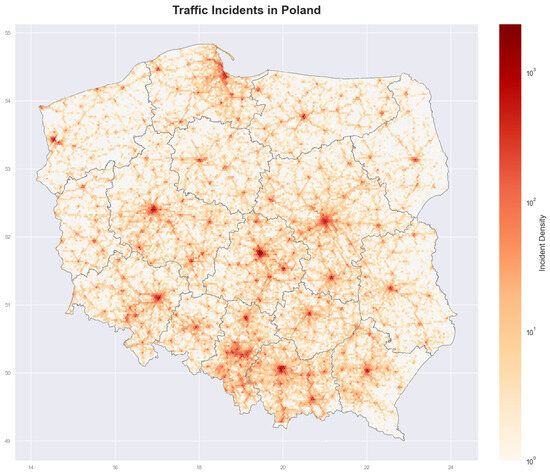
Figure 3.
Spatial distribution of traffic incidents across Poland. The heatmap displays incident density on a logarithmic scale, with brighter orange-red areas indicating higher concentrations of traffic incidents. Major urban centers, including Warsaw, Kraków, Łódź, Wrocław, and the Silesian metropolitan area, show distinctive hotspots, while the national road network is clearly visible through elevated incident frequencies along major transportation corridors.
Weather data marked with ⧫ were obtained by interpolating the conditions at the incident location based on the nearest available data, which includes temperature and humidity recorded at 10-minute intervals and precipitation recorded hourly, with the 24-hour precipitation calculated as the interpolation of the sum of previous hourly precipitation recordings. The interpolation process also incorporated elevation data (marked with ★) from GISCO’s Digital Elevation Model to account for altitude effects on weather conditions.
The weather variables in the dataset include temperature, representing air temperature in Celsius degrees; humidity, showing the relative humidity percentage at the incident site; and precipitation measures (precipitation_hourly and precipitation_cumulative), which provide the 1 h and 24 h accumulation in millimeters, respectively.
The sociodemographic indicators (marked with ▲) were obtained from GUS and assigned at the county level. For each incident, we incorporated statistics from the specific year when the incident occurred and from the county where it took place. These variables provide contextual information about local transportation infrastructure, vehicle fleet composition, and historical incident patterns.
Table 2 presents daily weather conditions aggregated at the county level. These data were also generated using kriging interpolation, but with the geographical center of each county serving as the target locations. This approach provided a consistent and representative meteorological view across all counties, enabling analysis of weather patterns at a specific administrative level while ensuring a fair reflection of typical weather conditions in each region. Daily averages were calculated for temperature and humidity, while precipitation values represent total daily accumulation.
Table 2.
Historical weather data.
Table 3 presents socioeconomic indicators from GUS organized hierarchically by year across different administrative levels (counties, voivodeships, and national level). The data include infrastructure metrics (road lengths and quality), vehicle fleet composition (by vehicle type), and historical accident statistics, providing important context for understanding regional differences. Population-normalized indicators such as road density per area and per capita were included to facilitate meaningful comparisons across administrative units of varying size and population.
Table 3.
Socioeconomic data by administrative unit.
2.4. Data Preprocessing
Data preprocessing is a critical step in constructing a reliable analytical dataset from diverse raw data sources. This process involves standardizing formats, addressing inconsistencies, and establishing spatial and temporal connections between data sources.
To determine the weather conditions for individual counties, central geographic coordinates of each county are extracted from the National Register of Boundaries (PRG) county dataset. These centroids serve as reference points for estimating meteorological conditions within each county.
Accurate kriging interpolation requires geographic data to be represented in a coordinate system that preserves distance relationships. Therefore, geographic coordinates were transformed from the WGS84 geographic coordinate system (EPSG:4326) to the Poland CS92 projected coordinate system (EPSG:2180), which is optimized for Poland’s territory. This transformation enables the kriging algorithm to properly account for the spatial distribution of weather stations relative to points of interest.
To ensure accurate temporal alignment between accident records and meteorological data, a rounding function is applied to incident timestamps. This function maps each event to the nearest available weather measurement interval—10 min for temperature and humidity data and the nearest full hour for precipitation.
Elevation data, incorporated as a drift term to enhance the kriging algorithm’s accuracy, underwent a two-step integration procedure. The input elevation data were originally partitioned into tiles, each spanning 10 degrees of both latitude and longitude. Four of these tiles covering Poland’s territory were merged and then clipped using extreme geographical points as boundary constraints. The resulting unified elevation model was then sampled at both incident locations and county centroids to associate each point with its corresponding elevation value.
Precipitation plays a crucial role not only at the moment of an accident but also in the preceding hours, as residual moisture can influence road conditions. Even if no rainfall is recorded at the exact time of an incident, wet or slippery surfaces may persist due to earlier precipitation. To capture this effect, we introduced the variable precipitation_cumulative, which represents the cumulative rainfall over the 24 h preceding each accident. This value is computed using a sliding window algorithm applied to hourly precipitation data, summing the previous 24 hourly measurements for each timestamp in the dataset. By incorporating recent precipitation history, this approach provides a more comprehensive representation of potential weather-related hazards affecting road safety.
To prevent erroneous merging during county data integration, a compound key approach was implemented, combining county name and voivodeship for all joining operations. This was essential as multiple counties across Poland share identical names but exist in different voivodeships. Two distinct methodologies were employed for administrative unit association: for geographical data, voivodeships were assigned to counties through spatial joins between county centroids and voivodeships’ administrative boundary shapefiles from the PRG; for socioeconomic data, encoding-based administrative matching utilized the first two digits of the standardized seven-digit county identifier. This latter approach required treating identifiers as strings to preserve leading zeros, which contained critical positional information within the administrative hierarchy. The distinct methodologies—spatial joins for geographical data and encoding-based matching for socioeconomic data—were essential for facilitating county weather data interpolation through kriging, as well as for merging socioeconomic data with incident data and generating choropleth visualizations of regional indicators, ensuring accurate synthesis and proper identification of all data sources.
Data integration employed relational join operations across multiple dimensions: SEWIK incident records were merged with BRD Observatory data through shared identifiers, while incident-socioeconomic linkage utilized a three-key join strategy based on year, county, and voivodeship identifiers. For weather conditions at incident locations, interpolated values were calculated using the adjusted timestamps to perform universal kriging. Daily county-level weather parameters were derived by applying the same kriging methodology to weather station measurements at county centroids, incorporating mean daily averages for temperature and humidity that we calculated, while leveraging the already available daily precipitation measurements from the IMGW dataset without further processing.
A consistent missing data handling strategy is implemented by inserting NaN markers in cases where source data are unavailable or interpolation algorithms fail to generate reliable estimates. This approach preserves analytical integrity by explicitly flagging incomplete records rather than introducing artificial values that could distort the analysis.
Outlier detection for weather parameters combines statistical methods with domain-specific constraints to ensure data quality. Extreme values are identified through distribution analysis of both input weather station data and resulting interpolated outputs. Manual review of the smallest and highest values in the dataset, supported by histogram visualization, helped identify questionable measurements. Physical limits—such as humidity constrained between 0 and 100% and non-negative precipitation—are enforced. To enhance meteorological plausibility, a minimum threshold is applied, classifying precipitation below 0.01 mm as zero, with this threshold being the minimum non-zero value observed in the input precipitation data. This combination of techniques ensures that only realistic and scientifically valid weather data are used in subsequent analyses.
By implementing rigorous data validation, interpolation, and quality control measures, we ensure that the processed dataset remains both reliable and analytically robust. These steps mitigate potential inaccuracies arising from missing values, outliers, and spatial inconsistencies, providing a solid foundation for further analysis of the relationship between weather conditions and road traffic incidents.
3. Results
3.1. Preprocessing Results
During the preprocessing phase, we encountered and resolved several data quality issues across our source datasets. These challenges required specific handling strategies to ensure data integrity and analytical validity.
In the socioeconomic dataset, we encountered challenges related to non-unique administrative unit names. Specifically, 10 county pairs, such as “powiat bielski,” shared identical names despite being located in different voivodeships. To prevent erroneous data merging, a compound key, comprising both the county and voivodeship names, was systematically employed. This approach was necessary for approximately 5% of the records to ensure unambiguous joins.
A further complication arose from inconsistent naming conventions for administrative units across different data sources. We found that 17% of county names required prefix standardization. This was primarily addressed by removing prefixes such as “m.” and “m. st.” from urban county designations, for instance, converting “powiat m. Bielsko-Biała” to “powiat Bielsko-Biała”. Additionally, temporal discontinuities required explicit handling. The urban county of Wałbrzych, for example, had distinct entries for different time periods (“powiat m. Wałbrzych od 2013” and “powiat m. Wałbrzych do 2002”), which were unified into a single record. A similar issue was observed with karkonoski county, which appeared under its former name, “powiat jeleniogórski”, in datasets predating 2021. This discrepancy, affecting approximately 0.2% of records, was resolved by standardizing to the current official name. These comprehensive standardization procedures collectively impacted 18% of all records in the socioeconomic dataset, ensuring consistency in subsequent preprocessing steps.
For the weather parameters, outlier detection was applied to identify and remove physically implausible or erroneous values. Temperature data falling outside the historically observed range for Poland (−41 °C to 50 °C) were excluded. Relative humidity values were constrained to the physically meaningful range of 0–100% through clipping. For precipitation, a statistical approach was employed: the histogram of recorded values was analyzed, and based on both the distribution and typical maximum values observed in Poland, outliers falling outside a plausible range were removed. Values below 0.01 mm, representing the minimum detectable precipitation threshold in the IMGW dataset, were set to zero to account for measurement precision limitations, affecting approximately 10.5% of records. These quality control procedures resulted in missing values in the final dataset for temperature (0.11%), precipitation (0.19%), and 24 h precipitation (0.17%), primarily due to outlier removal and occasional algorithm estimation failures.
Overall, preprocessing operations improved data quality while preserving most records, with less than 1% of the original dataset being excluded or substantially modified. Following standardization, socioeconomic indicators exhibited no significant outliers, and the visual inspection of the distributions before and after preprocessing confirmed that the transformations preserved the expected regional patterns across Poland. Similarly, weather-related variables demonstrated consistency with anticipated trends after outlier removal, further supported by visual validation of distributions’ integrity.
3.2. Kriging Results
Ordinary kriging was compared against universal kriging with elevation drift to determine whether the latter, despite its higher computational demands, was necessary for our analysis. Comprehensive cross-validation experiments were conducted on 100 randomly selected timestamps from the study period. For all evaluation strategies, multiple error metrics were calculated, including Root Mean Square Error (RMSE), Mean Absolute Error (MAE), and their normalized counterparts (NRMSE and NMAE) using the interquartile range (IQR) normalization. The interquartile range, representing the difference between the 75th and 25th percentiles of the data, provides a robust measure of variability that is less sensitive to outliers than standard deviation. This validation approach enabled quantitative assessment of interpolation accuracy across diverse meteorological conditions and spatial configurations.
The first evaluation strategy employed a nationwide comparison where a fraction of randomly selected weather stations (20%, equal to 96 sites) were used as reference points, with the remaining stations (80%, equal to 387 sites) serving as input data. The results of this approach, as presented in Table 4 and Figure 4, assessed the overall performance of both kriging methods across Poland’s entire meteorological network, encompassing diverse topographical and climatic conditions.
Table 4.
Nationwide comparison of universal and ordinary kriging methods based on cross-validation results using multiple error metrics.
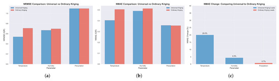
Figure 4.
Cross-validation performance comparison between universal and ordinary kriging methods across meteorological parameters using nationwide station data. (a) Normalized Root Mean Square Error (NRMSE) demonstrating universal kriging’s superior accuracy for temperature and humidity interpolation. (b) Normalized Mean Absolute Error (NMAE) confirming universal kriging’s consistent performance advantage across parameters. (c) Percentage improvement in NMAE achieved by universal kriging, with substantial gains for temperature (20.0%) and moderate improvements for humidity (4.3%), while precipitation shows minimal difference between methods (0.7%) favoring ordinary kriging.
The second evaluation strategy focused specifically on mountainous counties, where topographical influences on meteorological variables are most pronounced, and therefore where differences between kriging methods are expected to be substantial, as presented in Figure 5. This targeted analysis used a fraction of stations (20%, equal to 10 sites) from six selected high-elevation counties (tatrzański, nowotarski, suski, żywiecki, limanowski, and myślenicki) as reference points, while maintaining input data from the rest of the stations in the region. This configuration tested the methods’ ability to predict values in topographically complex terrain where elevation effects are most critical.
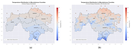
Figure 5.
Temperature distribution in mountainous counties of southern Poland using two kriging interpolation methods. (a) Ordinary kriging interpolation showing temperature patterns without accounting for elevation effects. (b) Universal kriging interpolation with elevation drift, demonstrating how temperature varies with topography. The maps display spatial temperature variation at a specific time across six counties: żywiecki, suski, nowotarski, tatrzański, limanowski, and myślenicki. Universal kriging reveals a strong temperature–elevation relationship, with colder temperatures at higher elevations, and exhibits better alignment with station measurements compared to ordinary kriging.
The results, as presented in Table 5 and Figure 6, demonstrated that incorporating topographical influences through universal kriging provided substantial benefits, particularly in mountainous regions where elevation significantly affects meteorological variables. The comparison revealed notable differences between the two methods, with universal kriging capturing gradients with considerably greater precision in topographically complex terrain. These findings confirmed that elevation-informed interpolation represents spatial variations more realistically, justifying the use of universal kriging despite increased computational costs.
Table 5.
Comparison of universal and ordinary kriging methods in mountainous counties based on cross-validation results using multiple error metrics.
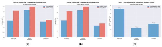
Figure 6.
Cross-validation performance comparison between universal and ordinary kriging methods in mountainous counties of southern Poland. (a) Normalized Root Mean Square Error (NRMSE) demonstrating universal kriging’s superior accuracy in topographically complex terrain, particularly for temperature interpolation. (b) Normalized Mean Absolute Error (NMAE) showing consistent performance improvements across all meteorological parameters when accounting for elevation effects. (c) Percentage improvement in NMAE achieved by universal kriging in mountainous regions, with substantial gains for temperature (35.4%), humidity (11.6%), and precipitation (16.7%), highlighting the critical advantage of incorporating elevation drift in complex topographic environments where terrain significantly influences meteorological patterns.
The kriging implementation encountered several technical limitations that required careful handling to ensure robust interpolation results. Some attempts produced singularity errors, most commonly when estimating precipitation in low-variance conditions. This occurred primarily when all weather stations within the interpolation domain reported nearly identical values—a frequent scenario with precipitation readings. Our solution implemented a two-tiered approach to handle problematic interpolation scenarios. For cases of complete uniformity, where all values were exactly equal—occurring in approximately 8% of precipitation interpolation cases—the algorithm bypassed kriging computation entirely and directly assigned the uniform value to interpolation targets. For scenarios with minimal but detectable variation, which affected 1.2% of precipitation metric cases, the implementation switched to using the pseudo-inverse of the kriging matrix. This approach enhanced numerical stability and successfully completed the interpolation despite increased computational costs. Temperature and humidity parameters did not require these fallback mechanisms and were processed using standard kriging methods throughout the interpolation process.
Overall, the universal kriging approach successfully generated continuous weather surfaces that respected both the spatial configuration of measurement stations and the topographical influences on weather patterns (Figure 7 and Figure 8). The interpolated values showed reasonable spatial coherence and aligned with expected meteorological patterns across Poland’s terrain.
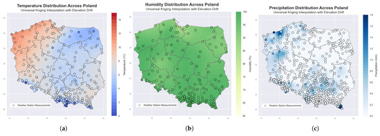
Figure 7.
Universal kriging interpolation of meteorological variables across Poland at a specific time, incorporating elevation as a drift term. Maps show interpolated values for (a) temperature (°C), (b) humidity (%), and (c) precipitation intensity (mm). Elevation-informed kriging highlights spatial patterns, especially in the mountainous southern regions where elevation significantly influences the variables.
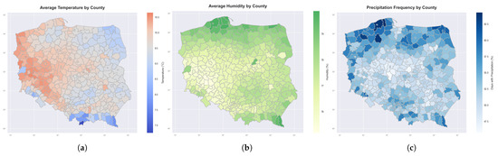
Figure 8.
Average weather conditions across Polish counties. The histograms display the following: (a) mean temperature (°C), (b) mean relative humidity (%), and (c) precipitation frequency (%). All meteorological variables were interpolated at county centroids using universal kriging from weather station data. Temperature and humidity are presented as daily averages, while precipitation frequency represents the percentage of days with total precipitation exceeding 0.1 mm.
3.3. Dataset
The dataset constructed for this study provides a comprehensive resource for examining the relationship between road traffic accidents (RTAs) and meteorological conditions. It comprises three primary groups of features: accident characteristics, meteorological parameters, and socioeconomic data. Accident attributes include precise location and timing information alongside detailed site characteristics such as road geometry, surface conditions, speed limits, and intersection types. Each incident record contains administrative location data from municipality to voivodeship level.
Meteorological variables encompass temperature, humidity, and precipitation measurements at both hourly and cumulative 24 h intervals for each accident location. Additionally, seasonal weather patterns for each county were captured through daily interpolated measurements, enabling analysis of meteorological trends in relation to incident frequency across administrative regions. These values were derived through universal kriging interpolation from weather station data.
Socioeconomic factors include indicators such as population density, transportation infrastructure metrics (road density, surface quality), vehicle fleet composition, and historical accident statistics. These variables provide essential baseline context for understanding regional risk patterns and normalizing accident rates across administrative units of varying sizes and development levels.
Figure 9 illustrates the distributional differences between general weather conditions and those during traffic incidents. The temperature histogram reveals that traffic incidents occur disproportionately during warmer conditions, while the humidity distribution shows fewer incidents at the highest humidity levels compared to the background weather distribution. The precipitation comparison demonstrates broadly similar patterns, with a slight underrepresentation of incidents during minimal precipitation conditions.
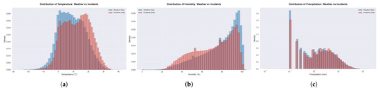
Figure 9.
Distribution comparison of weather parameters between all weather station measurements (blue) and weather conditions during traffic incidents (red). Incident data were interpolated using universal kriging. (a) Temperature distribution shows incidents occurring more frequently at higher temperatures compared to average weather conditions. (b) Humidity distribution. Incidents show a comparatively smaller peak at the highest humidity levels. (c) Precipitation distribution demonstrates similar patterns between general weather and incident conditions, with a notably lower number of incidents at the lowest registered precipitation.
As shown in Table 6, temperature values in the incident data range from −19.9 °C to 36.0 °C (mean 12.6 °C), while historical weather temperatures range from −22.0 °C to 36.0 °C (mean 9.6 °C). Humidity during incidents spans from 9.6% to 100% (mean 71.5%), compared to the historical range of 4.4% to 100% (mean 77.4%). Precipitation at incident times rarely exceeds 0.1 mm, with 75% of incidents occurring in conditions with no measurable precipitation.
Table 6.
Weather data statistics in the dataset.
The spatial distribution of incidents, both raw and normalized by different socioeconomic factors, provides insights into regional accident patterns, as illustrated in Figure 10. The raw incident count shows concentration in urban centers. However, normalizing by population density reveals higher per-capita incident rates, particularly in and around major urban areas. When normalized by vehicle ownership, the pattern shifts again, displaying a more even distribution with only a few focal points. The road infrastructure normalization identifies counties with high incident rates per kilometer of paved road and most closely resembles the original low-incident map, suggesting a less significant relationship between road infrastructure and incident occurrence.
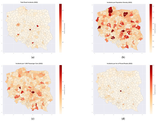
Figure 10.
Spatial distribution of road incidents in Poland in 2022, both direct and normalized by different socioeconomic factors. (a) Total road incidents across Polish counties. (b) Incidents per population density (incidents per person/km²) showing the distribution when accounting for population concentration. (c) Incidents per 1000 passenger cars displaying the relationship between incidents and vehicle ownership across counties. (d) Incidents per kilometer of paved roads illustrating incident rates relative to road infrastructure.
Our dataset allows for multi-scale correlation analyses between meteorological conditions and accident patterns. Figure 11 presents these correlations at both weekly and yearly temporal scales, revealing distinct relationships.
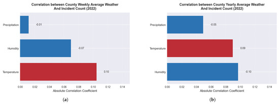
Figure 11.
Correlation between weather parameters and traffic incident counts at county level across different time scales. (a) Weekly correlations reveal that temperature has a positive association with incidents (0.10), while humidity (−0.07) shows a negative relationship and precipitation (−0.01) has almost no impact. (b) Yearly analysis demonstrates that humidity has the strongest negative correlation (−0.10), with temperature maintaining a positive association (0.09) and precipitation showing a moderate negative correlation (−0.05).
The multi-temporal analysis reveals how weather-incident relationships manifest differently across time scales. Weekly correlations highlight immediate effects of meteorological conditions on traffic safety, with temperature emerging as the most influential factor. In contrast, yearly correlations demonstrate persistent patterns where humidity assumes greater importance in the long-term relationship with incident rates.
Figure 12 presents correlation coefficients between accident metrics and various socioeconomic indicators at the county level. These correlations highlight key differences between factors influencing accident frequency versus severity. Fatality correlations generally show weaker associations compared to those for total accidents. Road infrastructure elements emerge as the most significant factors related to fatalities, while vehicle-related factors strongly dominate the correlations for total accidents, though they remain relevant for fatalities as well. Interestingly, both population density and municipal roads per 10,000 inhabitants demonstrate inverse relationships—showing minimal correlation with fatalities but considerably stronger associations with total accidents. These patterns suggest that distinct mechanisms likely underlie accident occurrence versus accident severity.
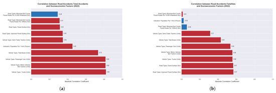
Figure 12.
Correlation coefficients between (a) road accident fatalities and (b) total accidents with socioeconomic factors at county level (2022). The figures reveal distinct patterns: fatality correlations are generally weaker than those for total accidents. For fatalities, improved paved surfaces and paved roads show the strongest associations (both 0.57), followed closely by vehicle types (trucks and motor vehicles at 0.56, passenger cars at 0.54). For total accidents, vehicle-related factors dominate with stronger correlations—trucks, motor vehicles, and passenger cars at 0.82 each, and buses at 0.73. Population density shows inverse relationships: slightly negative for fatalities (−0.02) but strongly positive for total accidents (0.45). Similarly, municipal roads per 10,000 inhabitants demonstrates negligible correlation with fatalities (0.01) but exhibits a substantial negative association with total accidents (−0.29).
This dataset provides a foundation for multiple analytical approaches in traffic safety research. Future applications include spatiotemporal risk modeling, infrastructure planning optimization, and policy effectiveness evaluation. The data particularly support Bayesian inference methods, as demonstrated in our related work [43]. The comprehensive collection of variables offers researchers a robust basis to investigate the complex relationships between traffic incidents, weather conditions, and socioeconomic factors.
4. Discussion
This study introduces a novel, integrated dataset to advance the analysis of road safety dynamics in Poland. Unlike traditional sources such as SEWIK, STATS19 (UK), or BAAC (France), which rely solely on police-reported accident data, our dataset incorporates these records with spatially interpolated meteorological measurements and sociodemographic indicators. Key variables are unified into a single table to simplify analysis while maintaining detail. Unlike global datasets like IRTAD, which offer only aggregated statistics, our micro-level approach enables fine-grained spatial and temporal analyses. To address challenges in linking localized weather conditions to accident sites, we employed universal kriging with elevation drift, producing terrain-aware weather surfaces—particularly valuable in Poland’s topographically diverse southern regions.
While the dataset represents a significant step forward in integrating diverse sources of information for road safety analysis, certain limitations remain. The accuracy of interpolated meteorological data is influenced by the spatial distribution and density of weather stations, which is particularly challenging for highly variable factors like precipitation. Additionally, socioeconomic data aggregated at the county level may mask local disparities within counties, such as differences between urban and rural communities. These sources of uncertainty should be considered when interpreting results.
The analytical potential of this integrated dataset is demonstrated by initial correlational analyses. Distinct patterns emerge in the relationships between accidents and various factors. Meteorological analyses revealed that temperature exhibits a positive association with incident counts (correlation coefficient 0.10 weekly, 0.09 yearly), while humidity shows a negative relationship (−0.07 weekly, −0.10 yearly), and precipitation demonstrates a negligible impact at the weekly scale (−0.01) but a moderate negative correlation yearly (−0.05). Regarding sociodemographic factors, the data suggest that different elements influence accident frequency versus severity: vehicle-related factors (trucks, motor vehicles, and passenger cars, all with correlations of 0.82) showed strong positive associations with total accident numbers, whereas improved road infrastructure correlated more significantly with fatalities (0.57). Population density presented an inverse pattern—negligible correlation with fatalities (−0.02) but strong positive association with total accidents (0.45). While these correlations do not imply causation, they collectively suggest that accident occurrence and severity may be driven by separate mechanisms. Although some of the mentioned correlations are weak, they can still provide useful information in multivariate predictive models. When combined with other factors, they may contribute to improved model performance through interaction effects or additive contributions. Additionally, small but consistent effects can be important in large-scale analyses where even subtle trends may influence decision-making.
Even at this preliminary stage, before applying advanced prognostic methods, the dataset offers valuable insights for road safety interventions. By integrating previously disparate data sources, it provides comprehensive contextual information that was unavailable when analyzing these sources separately. The weather–incident correlations can already inform targeted safety campaigns, suggesting enhanced monitoring during warmer periods when incident rates increase as well as improved driver education about visibility challenges in varying humidity conditions. The strong association between vehicle fleet composition and accident totals points to the need for enhanced vehicle safety standards and inspection programs, while the relationship between road infrastructure quality and fatalities suggests that improvement projects should prioritize roads with high fatality rates rather than high accident frequency alone. These differentiated approaches could help authorities allocate limited resources more effectively to reduce both accident numbers and their human cost.
Despite efforts to enhance spatial precision through kriging with elevation drift, certain challenges persist due to the inherent nature of meteorological data and the scale of socioeconomic indicators. In regions with sparse station coverage, interpolation may fail to capture localized weather events such as sudden downpours, fog formation, or microclimatic temperature shifts. These limitations are especially pronounced for precipitation, which is not only spatially erratic but also temporally dynamic, often varying significantly even within short timeframes and small areas. While our approach accounts for terrain effects, it cannot fully overcome the data scarcity problem. Additionally, precipitation is treated in this work as a single variable without distinguishing between rainfall, snowfall, or hail, due to limited data availability. Integrating supplementary sources such as weather radar or satellite-based observations could improve both spatial and temporal resolution in future iterations and allow for more nuanced differentiation between types of precipitation and their specific impacts. Similarly, the use of county-level socioeconomic data—though suitable for national-scale analysis—may obscure important intra-county variation. A single county may contain both high-density urban environments with heavy traffic and sparsely populated rural areas with different risk profiles, infrastructure quality, and road usage patterns. Without more fine-grained data, such heterogeneity cannot be fully addressed, potentially limiting the sensitivity of subsequent analyses.
The dataset’s structure positions it as a resource for advanced analytical frameworks, including Bayesian mentioned in our related work [43]. These methods can quantify probabilistic relationships between weather extremes and accident severity, offering actionable insights for policy formulation. Future research should aim to incorporate real-time, localized traffic flow data to better capture the dynamic nature of road usage and congestion patterns. More granular socioeconomic data would allow for a more accurate assessment of how demographic and infrastructural disparities influence road safety outcomes, especially in mixed urban–rural regions. In addition, behavioral indicators such as historical records of speeding and impaired driving could help account for human factors that are often critical yet difficult to quantify in large-scale datasets. Integrating high-resolution numerical weather prediction models or satellite-derived data could improve spatial and temporal precision of meteorological inputs, particularly for short-lived or rapidly changing weather conditions. By bridging meteorological, infrastructural, and sociodemographic dimensions, this work provides a critical foundation for developing more effective, evidence-based strategies to reduce the burden of road traffic accidents in Poland.
Author Contributions
Conceptualization, Ł.F. and A.F.; methodology, Ł.F., A.F. and J.B.; software, Ł.F. and A.F.; validation, A.F. and J.B.; formal analysis, Ł.F.; investigation, Ł.F.; resources, J.B.; data curation, Ł.F.; writing—original draft preparation, Ł.F.; writing—review and editing, Ł.F., A.F., M.K. and J.B.; visualization, Ł.F.; supervision, J.B.; project administration, J.B.; funding acquisition, J.B. All authors have read and agreed to the published version of the manuscript.
Funding
This work was funded by AGH Subvention for Scientific Activity.
Institutional Review Board Statement
Not applicable.
Informed Consent Statement
Not applicable.
Data Availability Statement
The data presented in this study are available on Zenodo as: Faruga, Ł., Filapek, A., & Baranowski, J. (2025). Traffic Accident Analysis in Poland: Integrating Weather Data and Sociodemographic Factors [Data set]. Zenodo. https://doi.org/10.5281/zenodo.15731344. This dataset was derived from the following resources available in the public domain: [35,36,37,40,41,42].
Conflicts of Interest
The authors declare no conflicts of interest.
Abbreviations
The following abbreviations are used in this manuscript:
| RTA | Road Traffic Accident |
| WHO | World Health Organization |
| EU | European Union |
| ANN | Artificial Neural Network |
| SVM | Support Vector Machine |
| ARIMA | Auto Regressive Integrated Moving Average |
| IDW | Inverse Distance Weighting |
| KED | Kriging with External Drift |
| SEWIK | Accident and Collision Recording System |
| POBRD | Polish Road Safety Observatory |
| IMGW | Institute of Meteorology and Water Management |
| GUS | Statistics Poland |
| DEM | Digital Elevation Model |
| GISCO | Geographic Information System of the Commission |
| PRG | National Register of Boundaries |
| UTM | Universal Transverse Mercantor |
| ANN | Artificial Neural Network |
| DUI | Driving Under the Influence |
| RMSE | Root Mean Square Error |
| NRMSE | Normalized Root Mean Square Error |
| MAE | Mean Absolute Error |
| NMAE | Normalized Mean Absolute Error |
| IQR | Interquartile Range |
| UK | United Kingdom |
| BAAC | Bulletin of Analysis of Bodily Injury Accidents |
| IRTAD | International Road Traffic and Accident Database |
References
- WHO—Road Traffic Injuries. Available online: https://www.who.int/news-room/fact-sheets/detail/road-traffic-injuries (accessed on 17 February 2025).
- European Road Safety Observatory—Annual Accident Report 2022. Available online: https://road-safety.transport.ec.europa.eu/european-road-safety-observatory/statistics-and-analysis-archive/annual-accident-report_en (accessed on 17 February 2025).
- Chand, A.; Jayesh, S.; Bhasi, A.B. Road traffic accidents: An overview of data sources, analysis techniques and contributing factors. Mater. Today Proc. 2021, 47, 5135–5141. [Google Scholar] [CrossRef]
- Abohassan, A.; El-Basyouny, K.; Kwon, T.J. Effects of Inclement Weather Events on Road Surface Conditions and Traffic Safety: An Event-Based Empirical Analysis Framework. Transp. Res. Rec. 2022, 2676, 51–62. [Google Scholar] [CrossRef]
- He, L.; Liu, C.; Shan, X.; Zhang, L.; Zheng, L.; Yu, Y.; Tian, X.; Xue, B.; Zhang, Y.; Qin, X.; et al. Impact of high temperature on road injury mortality in a changing climate, 1990–2019: A global analysis. Sci. Total Environ. 2023, 857, 159369. [Google Scholar] [CrossRef] [PubMed]
- Basagaña, X.; Escalera-Antezana, J.P.; Dadvand, P.; Llatje, Ò.; Barrera-Gómez, J.; Cunillera, J.; Medina-Ramón, M.; Pérez, K. High Ambient Temperatures and Risk of Motor Vehicle Crashes in Catalonia, Spain (2000–2011): A Time-Series Analysis. Environ. Health Perspect. 2015, 123, 1309–1316. [Google Scholar] [CrossRef] [PubMed]
- Park, J.; Choi, Y.; Chae, Y. Heatwave impacts on traffic accidents by time-of-day and age of casualties in five urban areas in South Korea. Urban Clim. 2021, 39, 100917. [Google Scholar] [CrossRef]
- Andersson, A.; Chapman, L. The use of a temporal analogue to predict future traffic accidents and winter road conditions in Sweden. Meteorol. Appl. 2011, 18, 125–136. [Google Scholar] [CrossRef]
- Basagaña, X.; de la Peña-Ramirez, C. Ambient temperature and risk of motor vehicle crashes: A countrywide analysis in Spain. Environ. Res. 2023, 216, 114599. [Google Scholar] [CrossRef] [PubMed]
- Fridstrøm, L.; Ifver, J.; Ingebrigtsen, S.; Kulmala, R.; Thomsen, L.K. Measuring the contribution of randomness, exposure, weather, and daylight to the variation in road accident counts. Accid. Anal. Prev. 1995, 27, 1–20. [Google Scholar] [CrossRef]
- Burke, P.J.; Nishitateno, S. Gasoline prices and road fatalities: International evidence. Econ. Inq. 2015, 53, 1437–1450. [Google Scholar] [CrossRef]
- Psarras, A.; Panagiotidis, T.; Andronikidis, A. The role of tourism in road traffic accidents: The case of Greece. Curr. Issues Tour. 2023, 27, 567–583. [Google Scholar] [CrossRef]
- Bellos, V.; Ziakopoulos, A.; Yannis, G. Investigation of the effect of tourism on road crashes. J. Transp. Saf. Secur. 2019, 12, 1–18. [Google Scholar] [CrossRef]
- Grabowski, D.C.; Morrisey, M.A. Do higher gasoline taxes save lives? Econ. Lett. 2006, 90, 51–55. [Google Scholar] [CrossRef]
- Castillo-Manzano, J.I.; Castro-Nuño, M.; López-Valpuesta, L.; Vassallo, F.V. An assessment of road traffic accidents in Spain: The role of tourism. Curr. Issues Tour. 2020, 23, 654–658. [Google Scholar] [CrossRef]
- Naqvi, N.; Quddus, M.; Enoch, M. Do higher fuel prices help reduce road traffic accidents? Accid. Anal. Prev. 2019, 135, 105353. [Google Scholar] [CrossRef]
- Quest, W.; Goodness, W.; Elly, B. Statistical Modeling of Road Traffic Accident Patterns and Prediction of Future Accident Hotspots. Preprint on ResearchGate. 2025. Available online: https://www.researchgate.net/publication/390096337_Statistical_Modeling_of_Road_Traffic_Accident_Patterns_and_Prediction_of_Future_Accident_Hotspots (accessed on 27 June 2025).
- Eisenberg, D.; Warner, K.E. Effects of Snowfalls on Motor Vehicle Collisions, Injuries, and Fatalities. Am. J. Public Health 2005, 95, 120–124. [Google Scholar] [CrossRef]
- Bergel-Hayat, R.; Debbarh, M.; Antoniou, C.; Yannis, G. Explaining the road accident risk: Weather effects. Accid. Anal. Prev. 2013, 60, 456–465. [Google Scholar] [CrossRef]
- Lee, W.K.; Lee, H.A.; Hwang, S.S.; Kim, H.; Lim, Y.H.; Hong, Y.C.; Ha, E.H.; Park, H. A time series study on the effects of cold temperature on road traffic injuries in Seoul, Korea. Environ. Res. 2014, 132, 290–296. [Google Scholar] [CrossRef]
- El-Basyouny, K.; Kwon, D.W. Assessing Time and Weather Effects on Collision Frequency by Severity in Edmonton Using Multivariate Safety Performance Functions. In Proceedings of the Transportation Research Board 91st Annual Meeting, Washington, DC, USA, 22–26 January 2012; Board, T.R., Ed.; ACM: New York, NY, USA, 2012. Available online: https://trid.trb.org/View/1128732 (accessed on 17 February 2025).
- Theofilatos, A.; Yannis, G. A review of the effect of traffic and weather characteristics on road safety. Accid. Anal. Prev. 2014, 72, 244–256. [Google Scholar] [CrossRef]
- Brijs, T.; Karlis, D.; Wets, G. Studying the effect of weather conditions on daily crash counts using a discrete time-series model. Accid. Anal. Prev. 2008, 40, 1180–1190. [Google Scholar] [CrossRef]
- Dirks, K.N.; Hay, J.E.; Stow, C.D.; Harris, D. High-resolution studies of rainfall on Norfolk Island: Part II: Interpolation of rainfall data. J. Hydrol. 1998, 208, 187–193. [Google Scholar] [CrossRef]
- Stow, C.D.; Dirks, K.N. High-resolution studies of rainfall on Norfolk Island: Part 1: The spatial variability of rainfall. J. Hydrol. 1998, 208, 163–186. [Google Scholar] [CrossRef]
- Berne, A.; Delrieu, G.; Creutin, J.D.; Obled, C. Temporal and spatial resolution of rainfall measurements required for urban hydrology. J. Hydrol. 2004, 299, 166–179. [Google Scholar] [CrossRef]
- Kebaili Bargaoui, Z.; Chebbi, A. Comparison of two kriging interpolation methods applied to spatiotemporal rainfall. J. Hydrol. 2009, 365, 56–73. [Google Scholar] [CrossRef]
- Delhomme, J.P. Kriging in the hydrosciences. Adv. Water Resour. 1978, 1, 251–266. [Google Scholar] [CrossRef]
- Goovaerts, P. Geostatistical approaches for incorporating elevation into the spatial interpolation of rainfall. J. Hydrol. 2000, 228, 113–129. [Google Scholar] [CrossRef]
- Phillips, D.L.; Dolph, J.; Marks, D. A comparison of geostatistical procedures for spatial analysis of precipitation in mountainous terrain. Agric. For. Meteorol. 1992, 58, 119–141. [Google Scholar] [CrossRef]
- Wu, T.; Li, Y. Spatial interpolation of temperature in the United States using residual kriging. Appl. Geogr. 2013, 44, 112–120. [Google Scholar] [CrossRef]
- Chung, U.; Yun, J.I. Solar irradiance-corrected spatial interpolation of hourly temperature in complex terrain. Agric. For. Meteorol. 2004, 126, 129–139. [Google Scholar] [CrossRef]
- Shtiliyanova, A.; Bellocchi, G.; Borras, D.; Eza, U.; Martin, R.; Carrère, P. Kriging-based approach to predict missing air temperature data. Comput. Electron. Agric. 2017, 142, 440–449. [Google Scholar] [CrossRef]
- Zarządzenie nr 31 Komendanta Głównego Policji z Dnia 22 Października 2015 r. w Sprawie Metod i Form Prowadzenia Przez Policję Statystyki Zdarzeń Drogowych [Order No. 31 of the Commander-in-Chief of Police of October 22, 2015, on the Methods and Forms of Maintaining Road Incident Statistics by the Police]. Available online: https://edziennik.policja.gov.pl/legalact/2015/85/ (accessed on 21 February 2025).
- Mapa wypadków—Polskie Obserwatorium Bezpieczeństwa Ruchu Drogowego [Accident Map—Polish Road Safety Observatory]. Available online: https://obserwatoriumbrd.pl/mapa-wypadkow/ (accessed on 17 February 2025).
- Non-Commercial Platform Providing Data from SEWIK. Available online: https://sewik.pl/search. (accessed on 17 February 2025).
- Publiczne Dane Pomiarowo Obserwacyjne IMGW [Public Measurement and Observational Data of IMGW]. Available online: https://danepubliczne.imgw.pl/data/dane_pomiarowo_obserwacyjne/ (accessed on 17 February 2025).
- Instytut Meteorologii i Gospodarki Wodnej—Państwowy Instytut Badawczy [Institute of Meteorology and Water Management—National Research Institute]. Available online: https://imgw.pl/strona-glowna/zadania-statutowe/ (accessed on 18 February 2025).
- Ośrodki i Stacje Pomiarowo-Obserwacyjne IMGW [Meteorological Centers and Stations of IMGW]. Available online: https://imgw.pl/strona-glowna/osrodki-i-stacje/ (accessed on 18 February 2025).
- Statistics Poland—Local Data Bank. Available online: https://bdl.stat.gov.pl/bdl/start (accessed on 17 February 2025).
- Eurostat—GISCO—Copernicus. Available online: https://ec.europa.eu/eurostat/web/gisco/geodata/digital-elevation-model/copernicus#Elevation (accessed on 17 February 2025).
- National Register of Boundaries. Available online: https://www.geoportal.gov.pl/en/data/national-register-of-boundaries/ (accessed on 1 March 2025).
- Filapek, A.; Faruga, Ł.; Baranowski, J. Bayesian Modeling of Traffic Accident Rates in Poland based on Weather Conditions. Appl. Sci. 2025. submitted. [Google Scholar]
Disclaimer/Publisher’s Note: The statements, opinions and data contained in all publications are solely those of the individual author(s) and contributor(s) and not of MDPI and/or the editor(s). MDPI and/or the editor(s) disclaim responsibility for any injury to people or property resulting from any ideas, methods, instructions or products referred to in the content. |
© 2025 by the authors. Licensee MDPI, Basel, Switzerland. This article is an open access article distributed under the terms and conditions of the Creative Commons Attribution (CC BY) license (https://creativecommons.org/licenses/by/4.0/).