Monitoring and Evaluating the Damage to Shear Connectors in Steel–Concrete Composite Beams by Curvature-Based Indicators Through Vibration Tests

Abstract

In order to assess the workability of shearing connectors of steel–concrete composite beams (SCCBs), this manuscript proposed a novel solid-slipping nonlinear finite element (FE) model, which is independent of stiffness-slip function for simply supported SCCBs. The modal curvature difference and the modal flexibility difference curvature were prompted, which are able to evaluate both sole-damage and multi-damage. It was concluded that the proposed indicators can locate the damaged shear studs and quantify the damage degree correctly, having a maximum error of less than 1%. Robust analysis proved that the proposed indicators are still highly precise when the noise level is up to 8%, which is highly significant for further practical application.

1. Introduction

The steel–concrete composite beam has achieved wide acceptance because it guarantees economic benefits, strength and stiffness improvement, and construction convenience and has been extensively used in modern high-rise buildings, stadiums, and bridges [1,2]. In steel–concrete composite beams, the connection between the steel beam and concrete slab is commonly provided in forms of welded shear studs, bolts, or perforated plates (Figure 1), among which the welded shear studs have become the most popularly used due to the availability of detailed research and standard design methodology. The shear connectors between the concrete slab and steel girder are often subjected to serious stress, overloading, corrosion, and fatigue. All these anomalies involve a deterioration or break of shear connectors, causing a decrease in the rigidity, a reduction in resistance, and catastrophic structural failures with huge losses.

Condition assessment for the local shear connectors in SCCBs is of great significance to ensure structural reliability and durability. However, the inaccessibility of the shear connectors makes direct visual inspection unusable. On the other hand, a huge number of shear connectors prevents any local Non-Destructive Testing (NDT) methods from being able to inspect the connectors one by one. From a great variety of NDT methods developed to date, the vibration-based method is recognized as one of the least expensive and simultaneously effective, with appropriate processing of measurement data. The premise of the vibration-based method is that the damage or deterioration of the structures would primarily affect the stiffness and thus the modal characteristics of structures, e.g., the natural vibration frequency [3], mode shapes [4,5], frequency response function, etc. [6]. Thus, damage can be inferred from the changes in identified dynamic properties.

Recently, methods based on changes in derived modal parameters such as modal strain energy, mode shape curvature, and flexibility have been considered more sensitive to damage than vibration frequency. Dilena et. al. [7] investigated the influence of shear stud damages on the dynamic characteristics of SCCBs and concluded that the bending modal is more sensitive to the damage of shear studs. Chellini et al. [8] conducted the finite element model updating based on vibration measurements to assess and quantify the structural damage of a high ductile steel–concrete composite frame. Brigante et. al. [9] proved the effectiveness of modal assurance criterion (MAC) in damage evaluation for concrete structures, and Gohar et al. [10] combined the modal damping ratio and coordinate modal assurance criteria (COMAC) to locate and evaluate the internal deterioration of reinforced concrete (RC) slabs at different loading stress through vibration-based tests. Mehboob et. al. [11] proposed a modified jerk energy methodology to localize the reduction in the stiffness of a reinforced concrete shear frame. Yin et. al. [12] proposed a vibration-based damage detection method for bolted connections using incomplete modal data by a Bayesian approach and model reduction technique.

To the author’s best knowledge, only a few studies concentrated on the detection of damage to shear connectors in SCCBs. Dilena et al. [3] applied the diagnostic methodology based on natural frequency and modal shapes to evaluate the damage to shear connectors of SCCBs. Hou et al. [4] proposed locating the damaged shear stud by comparing the changes in curvature modes before and after the damage occurred, but no quantitative evaluation was conducted. Xia and Li et al. [13,14] reported a damage assessment for a steel–concrete beam based on vibration data in the frequency domain. Damage indicators such as the correlation of FRFs (COFRF), the relative difference of FRFs (RDFRF), and transmissibility were proposed and validated. Akshat et al. [15] proposed a parameter estimation algorithm for updating the FE model for the damage assessment of reinforced concrete slabs using vibration-based frequency response function (FRF) data. Li et al. [16] proposed a dynamic condition assessment approach based on wavelet packet energy of cross-correlation functions from the recorded acceleration responses to identify the damage of shear studs in slab-on girders.

Although the vibration-based testing methodology for the damage detection of shear studs in SCCBs has gained much interest over the past years, there remains some debate as to whether the measured modal parameters are sensitive enough and suitable for detecting multiple instances of damage. This study focuses on quantifying the damage to shear studs in SCCBs by novel proposed modal-shape-based indicators. The contribution of the present study is threefold: (1) a novel solid-slipping nonlinear FE model for the SCCB is developed in ABAQUS 2021 without depending on the stiffness–slip function, to guarantee the accuracy of dynamic perturbation analysis; (2) two vibration-based indicators, namely the modal curvature difference and the modal flexibility difference curvature are proposed to locate the damaged shear studs and quantify the damage degree; (3) the robustness and sensibility of the two indicators were proven to drive further practical application.

2. Theoretical Backgrounds of Damage Detection with Modal Information

2.1. Modal Curvature Difference

In beam-type structures (Figure 2), by considering the force balance and deformation coordination at the interface of micro-segments, the curvature function at location x in flexural vibration is given as:

$${\displaystyle \frac{M}{EI(x)}}=k(x)$$

(1)

where M, E, and I(x) are the moment, modulus of elasticity, and moment of inertia of the section; k(x) is the curvature.

The curvature k(x) can be expressed as the reciprocal of the radius of curvature $\rho \left(x\right)$:

$${\displaystyle \frac{1}{\rho (x)}}={\displaystyle \frac{{\partial }^{2}u(x)}{\partial x^2}}={\displaystyle \sum _{n=1}^{\infty }{{\varphi }_n}^{″}(x)q(x)}$$

(2)

where u(x) is the displacement, φ_n″(x) is the nth curvature mode, and q(x) is the external load.

From Equations (1) and (2), the reduction in stiffness due to damage leads to an increase in modal curvature. Researchers have reported that the modal curvature is far more sensitive than other modal-based indicators such as the MAC and COMAC [17]. For beam-type structures, mainly subjected to bending deformation, the modal curvature can be calculated using the quadratic difference of normalized modal shapes. For the nth mode, the curvature at the ith node can be expressed as:

$$k(x)={\displaystyle \frac{{\varphi }_{n,i-1}-2{\varphi }_{n,i}+{\varphi }_{n,i+1}}{l^2}}$$

(3)

where ϕ_ni is the modal displacement at coordinate point i, for the nth mode, and l is the distance between two nearby coordinate points.

To calculate the curvature changes with respect to the undamaged state, the modal curvature difference can be calculated as in Equation (4):

$$\Delta V={\displaystyle \sum _{\mathrm{i}=1}^n\left|{\kappa }^d(x)-\kappa (x)\right|}$$

(4)

where ΔV, n, and κ(x) represent the absolute value of curvature difference, the number of modal shapes, and modal curvature, respectively; superscript d refers to the damaged state.

2.2. Modal Flexibility Difference Curvature

Structural stiffness refers to the ability of structures to resist deformation. The occurrence of local damage causes the degradation of stiffness; thus, the structural stiffness is a good indicator of structural damage (Equation (5)).

$$\left[K\right]={\displaystyle \sum _{i=1}^n{w}_i^2\left\{{\varphi }_i\right\}}{\left\{{\varphi }_i\right\}}^T$$

(5)

where $w$_i and ϕ_i represent the corresponding modal frequency and modal shape.

However, the stiffness matrix is significantly affected by the high-order modes, which causes difficulty in practical applications. Therefore, modal flexibility, which is defined as the reciprocal of stiffness, has been widely used for damage detection. The modal flexibility matrix can be calculated by Equation (6).

$$\left[f\right]=\mathrm{\Phi }{\Omega }^{-1}{\mathrm{\Phi }}^T={\displaystyle \sum _{i=1}^n\frac{1}{w_i^2}\left\{{\varphi }_i\right\}}{\left\{{\varphi }_i\right\}}^T$$

(6)

where Φ = [${\varphi }_1$, ${\varphi }_2$, ${\varphi }_3$, …] is the modal shape matrix, ${\varphi }_i$ is the mass-normalized mode shape, Ω = diag($w_i^2$) is the diagonal matrix composed of the squares of the natural frequency, $w_i$ is the ith natural frequency, and n is the number of modal shapes.

For two sets of measurements, the changes in the flexibility matrix can be calculated as:

$$\Delta ={\left[f\right]}_{\mathrm{d}}-{\left[f\right]}_{\mathrm{i}}$$

(7)

where [f]_d and [f]_i are the flexibility matrices for the damaged and intact cases.

For each measurement point j, let ${\overline{\delta }}_j$ be the maximum absolute value of the elements in the corresponding column of Δ, i.e.,

$${\overline{\delta }}_j=\underset{i}{\max }\left|{\delta }_{ij}\right|$$

(8)

where ${\overline{\delta }}_j$ is the quantity of alterations of flexibility for each measurement location, and ${\delta }_{ij}$ is the element of the jth column of Δ.

Further, the flexibility difference curvature can be calculated by the central difference method, as shown in Equation (9):

$${\overline{\delta }}_j^{″}={\displaystyle \frac{{\overline{\delta }}_{j-1}-2{\overline{\delta }}_j+{\overline{\delta }}_{j+1}}{l^2}}$$

(9)

where ${\overline{\delta }}_j^{″}$ is the flexibility difference curvature at point j, which is more sensitive to micro damages in SCCBs; l is the distance between adjacent measurement nodes; ${\overline{\delta }}_j$ is the flexibility difference at point j.

3. Modeling of the Steel–Concrete Composite Beam

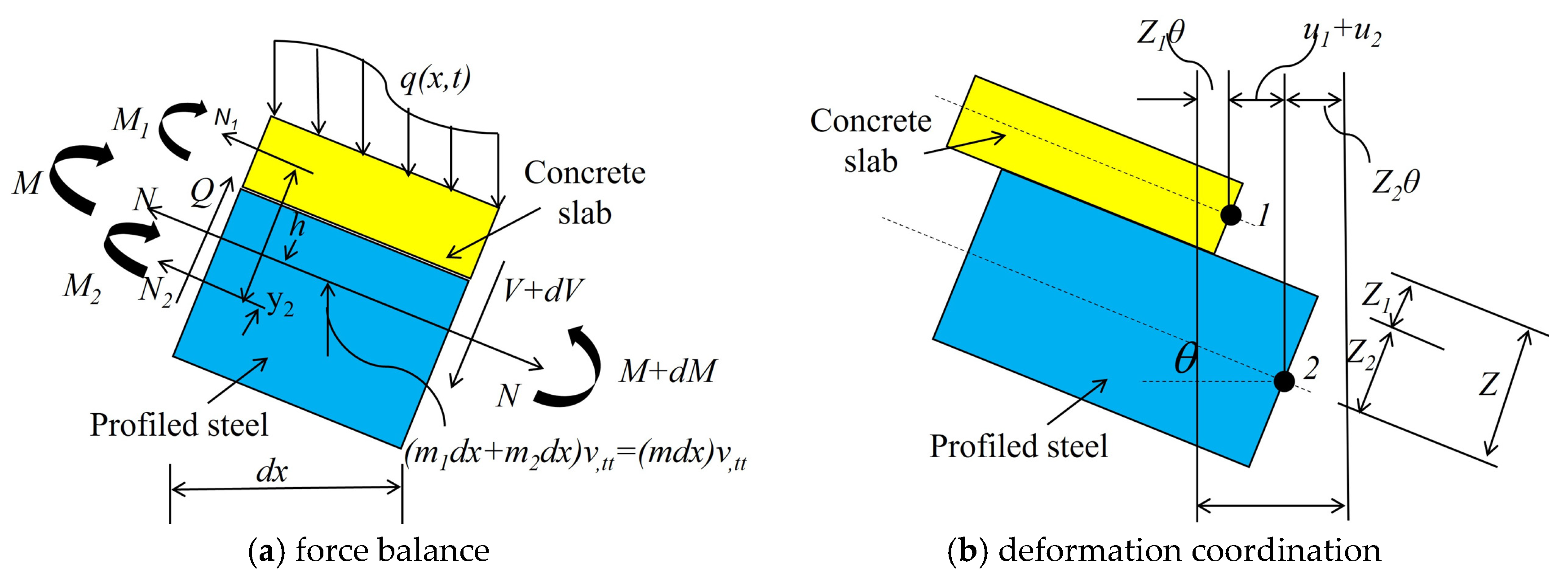
3.1. The Solid-Slipping Beam Model

To simulate the spatial stress and nonlinearity of SCCB, the Traditional Beam Model (TBM) method has been widely utilized [18]; however, the TBM assumes that the concrete slab and steel beam work together and simulates shear connectors by setting the stiffness function of spring elements or truss elements, which cannot reflect the slight changes in shear connectors and the surrounding concrete. In recent years, the solid-slipping beam model (SSBM) was favored by researchers due to its superiority in escaping the dependence on the stiffness-slip function [19]. To construct the SSBM for steel–concrete beams, the formulation of the model geometry, element types, material behavior, and solution technique is challenging; detailed descriptions are outlined as follows:

(1) Element types and meshes

To simulate the local stress effects of shear studs and surrounding concrete, the 8-node linear brick element (C3D8R) was proposed for concrete slab, steel beam, and headed shear studs. The 8-node linear brick is a reduced-integration solid continuum element with a Gauss integration point and is less prone to shear self-locking under bending load. Moreover, the hexahedral element has a better convergence rate than other solid elements, and the calculation accuracy is not significantly affected by sensitivity to mesh orientation. The T3D2 truss element with two nodes and three translational degrees of freedom was proposed for steel bars. The steel truss was embedded into the concrete slab, and no moments or forces perpendicular to the centerline were supposed. The T3D2 (truss) and C3D8R (brick) elements were connected by tie constraints, where the relative slip between steel bars and surrounding concrete was ignored.

All entities were sliced according to the principles of symmetry and deformation compatibility. To ensure good meshing quality and reduce the hourglassing effect, the structured grid technology and advancing front algorithm were adopted, and the hourglass control option in ABAQUS was enabled. Additionally, a refined grid for the headed shear studs and surrounding concrete was conducted, which will be detailed in Section 3.2, Section 3.3, and Section 4.1.

(2) Material modeling

Concrete has significant anisotropy and stress complexity. The concrete damaged plasticity (CDP) model has been proven to be a granted choice because the CDP model can reflect the mechanical properties of concrete under both tensile and compressive stress and handle local stress concentration effectively [20,21]. In this study, the CDP model was adopted for concrete when conducting the mechanical performance analysis in the corresponding sub-section.

In the CDP model, the nonlinear (elastic-plastic) mechanical behavior of the concrete was presented by an equivalent uniaxial stress–strain curve based on Euro Code 2 (EC2) [22], as shown in Figure 3a. For concrete in compression, three parts of the curve can be identified. The first part was initially assumed to be linear elastic up to 0.4f_ck, where f_ck is the compressive cylinder strength of the concrete. The initial modulus of elasticity of the concrete was recommended by EC2, as in Equation (10). Poisson’s ratio of concrete is taken as 0.2.

E_cm = 0.95 × (f_ck + 8)^1/3 (E_cm in GPa, f_ck in MPa)

(10)

The second part of the curve was the non-linear parabolic portion starting from the proportional limit stress 0.4f_ck to the peak stress f_ck, which can be determined from Equation (11):

$${\sigma }_{\mathrm{c}}=\left({\displaystyle \frac{kn-n^2}{1+\left(k-2\right)n}}\right)f_{\mathrm{ck}}$$

(11)

where n = ε_c/ε_c1, ε_c1 represents the strain at peak stress (ε_c1 = 0.0022), and k = 1.1E_cm × ε_c1/f_ck; f_ck represents the compressive cube strength of the concrete.

The third part of the stress–strain curve was the linear descending part from f_ck to a value of rf_ck lower than or equal to f_ck. The reduction factor r is valued ranging from 0.5 to 1, depending on the concrete strength.

For concrete in tension, as illustrated in Figure 3a, the tensile stress was assumed to increase linearly with respect to the strain until cracking; thereafter, the tensile stress decreases linearly to zero with a tension stiffening effect coming into play. To avoid unstable and premature convergence, the ultimate strain was supposed to be taken as 0.005, i.e., β = 50 and ε_ck = 0.0001, by adopting the suggestions in the ABAQUS manual.

For steel and headed shear studs, a tri-linear stress–strain constitutive relationship was supposed to define the mechanical behavior under tension and compression, as shown in Figure 3b. The material shows initial elastic behavior up to its yielding point, followed by strain hardening and further yielding. The yield stress (σ_ys) was determined at ε_ys = 0.2% and the ultimate stress (σ_us) was achieved at ε_ps = 0.6%.

(3) Interaction, constraint, and boundary conditions

Once all components of the composite beam were properly positioned, the penalty contact method was adopted to simulate the surface–surface contact interactions between steel and concrete. The HARD contact property was supposed to depict the contact behavior in the direction normal to the interface plane, while the PENALTY option was supposed to specify the tangential response by adopting a proper friction coefficient. The “master” and “slave” surfaces of these interactions were designated by considering the meshing density and the material strength of the referred component, where the steel flange and headed stud were preferably designated as the “master” surface.

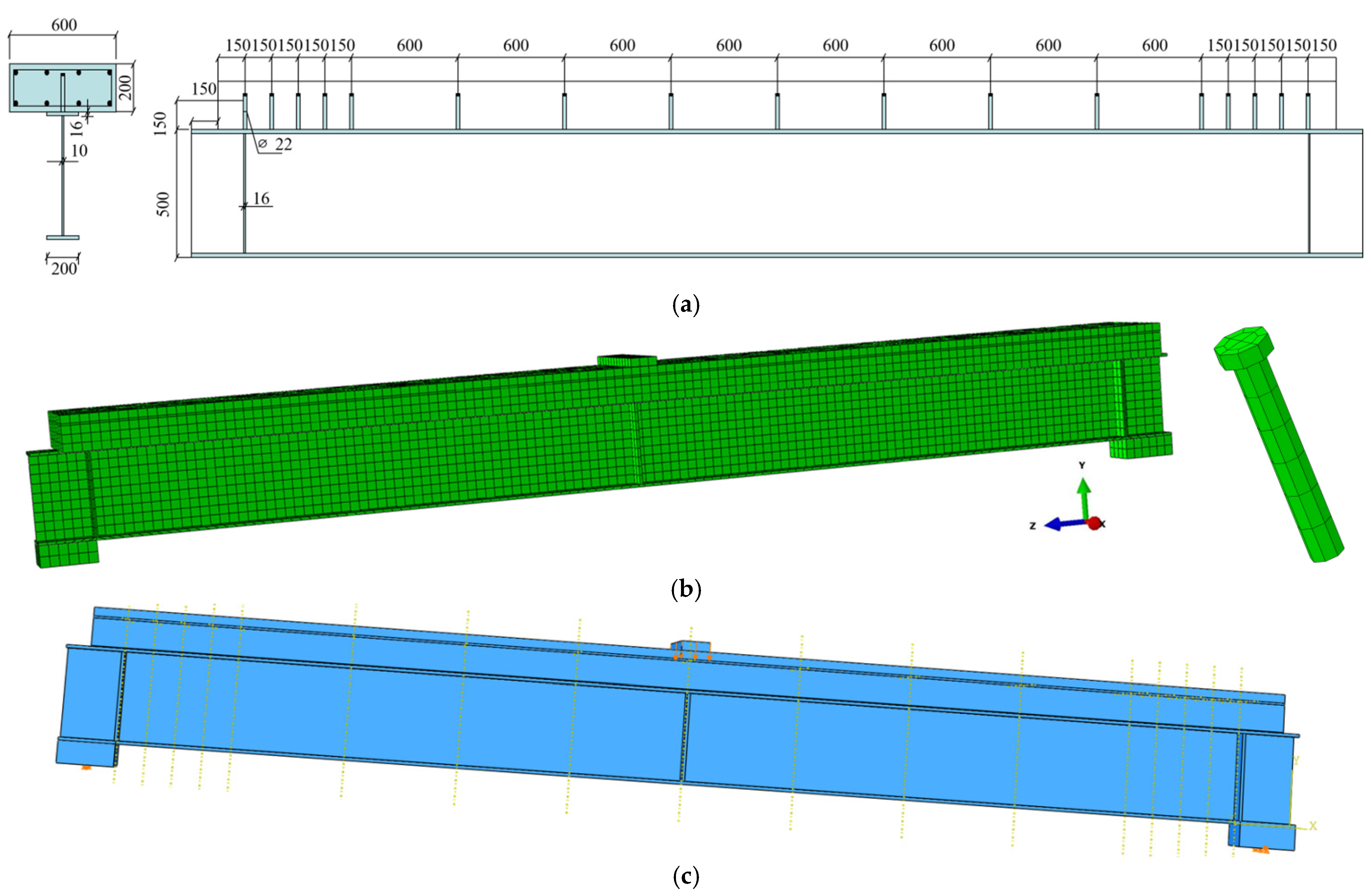
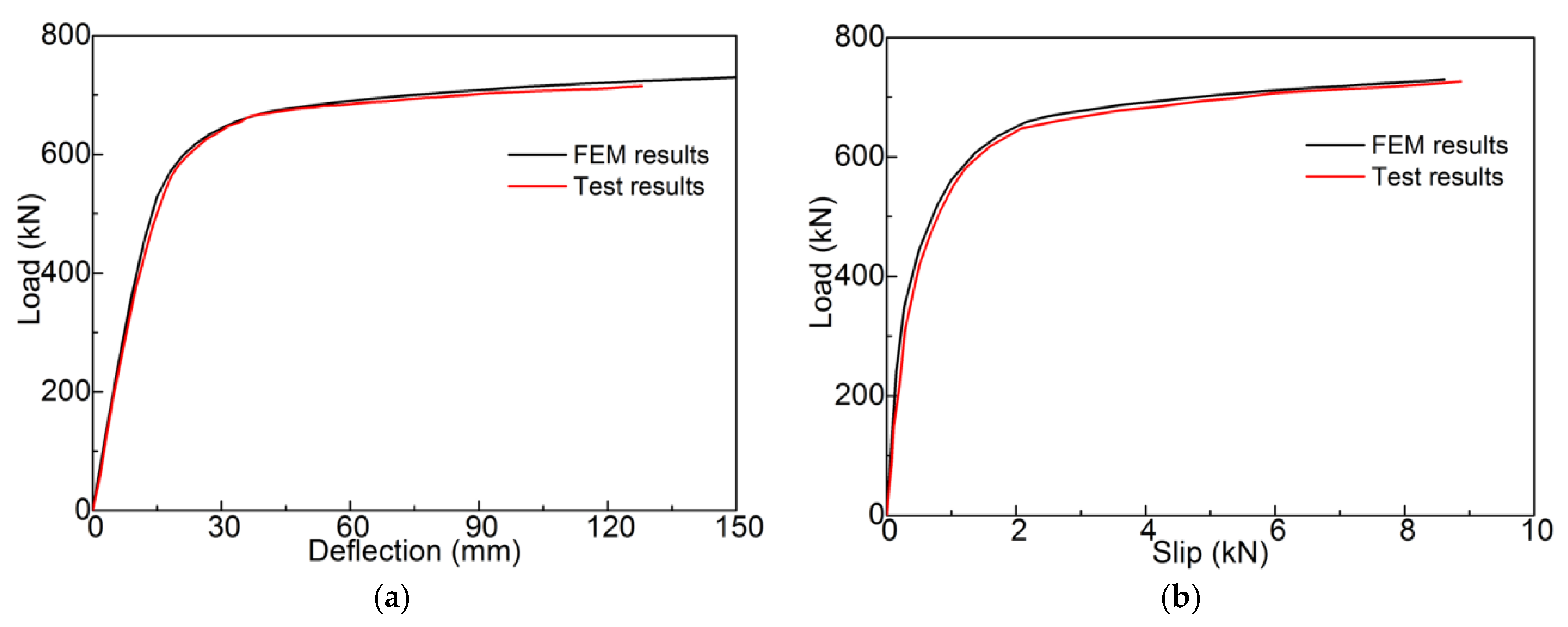
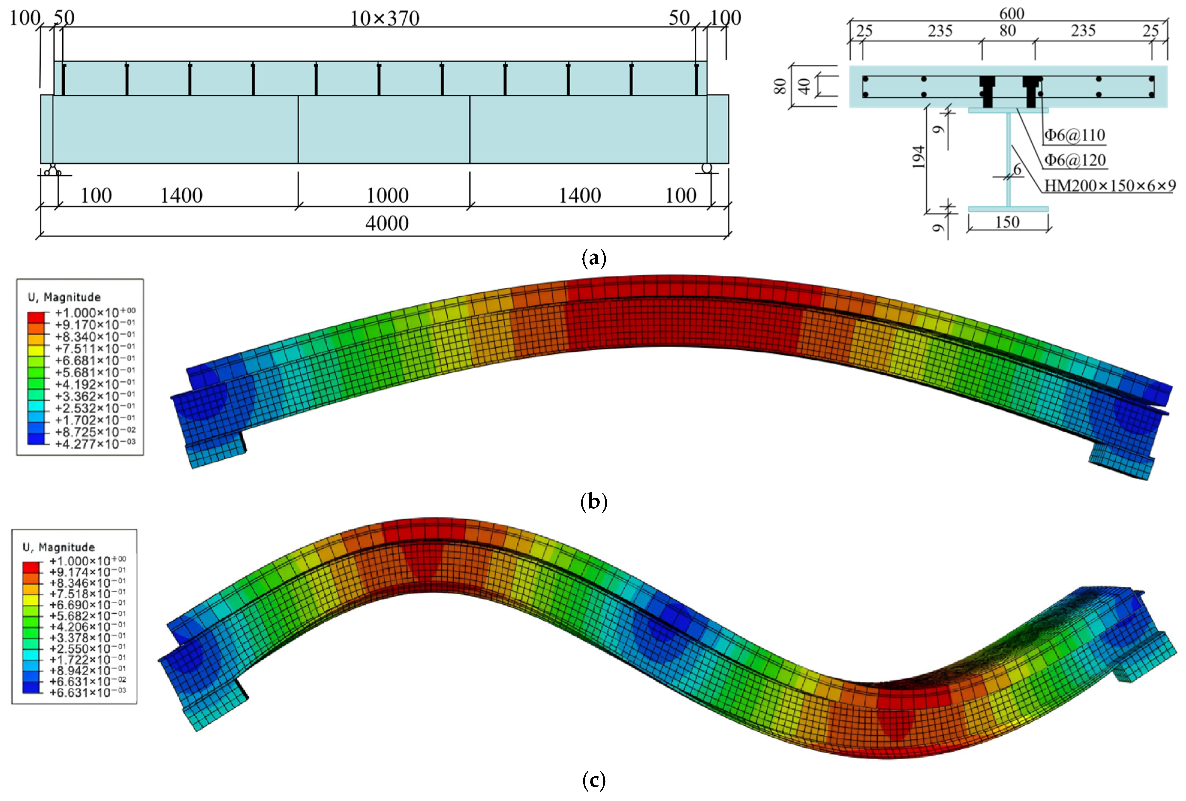
3.2. FE Model Verification 1

The first FE model presented herein was calibrated on the results of a three-point bending test conducted by Lee et al. [23]. The simply supported beam has a net span of 6300 mm and a total height of 700 mm. The headed studs have a diameter of 22 mm and a height of 150 mm. Detailed dimensions of the composite beam are shown in Figure 4a.

Table 1. Material properties of FE model 1.

Material	Yield Strength (MPa)	Tensile Strength (MPa)	Elastic Modulus (GPa)	Thickness or Diameter (mm)	Elongation
Steel beam	320	−	210	14	34%
Rebar	400	−	208	16	−
Headed stud	353	426	208	22	−
Concrete	−	49.4	36.68	−	−

provides the detailed properties of the materials. In the solid-slipping beam model, all material parameters were defined based on the actual material properties. The dilation angle and the eccentricity parameter for the CDP model were taken as 20° and 0.1, respectively, and the ratio of the biaxial compressive strength and the uniaxial compressive strength was taken as 1.16.

Figure 4b shows the three-dimensional finite element model developed in ABAQUS. A loading slab with the dimension of 60 × 150 × 50 mm and two supporting slabs with the dimension of 300 × 200 × 100 mm was modeled and tied to the upper surface of the concrete slab and the lower surface of steel flange, respectively, for the convenience of applying boundary conditions and avoiding over constraint. The initial elasticity modulus of the loading slab and supporting slab was valued at 1000 times that of the structural steel, to ensure the micro-distortion.

A general mesh size of 50 mm was defined for the overall structure, and a fine mesh size of 10 mm was adopted for the headed stud and the region around the head studs. The mesh sizes were also verified by carrying out the sensitivity analysis. Overviews of the finite element model and corresponding meshes are shown in Figure 4b, together with the coordinate system in which the X and Y axes define the cross-sectional plane, and the Z-axis is parallel to the longitudinal direction of the SCCB.

The simply supported condition was applied at the supporting slabs, which were tied to the end of the steel beam, for which the translational displacements in the X and Y directions were restrained. The static solving was realized in the STANDARD module, by controlling the mid-span downward enforced (–Y) displacement at a specific rate. The interface slip was measured as the relative displacement between the nodes on the steel flange and concrete slab. The exact value of loads was measured as the total reaction acting on the loading surface. All boundary conditions are shown in Figure 4c.

To simulate the damage process of SCCBs accurately, different friction coefficients have been tried; the most appropriate friction coefficients were determined as 0.1 for the interface between the steel flange and concrete slab and 0.45 for the surfaces of the headed studs and surrounding concrete. Figure 5 provides a comparison of the results of the experiment and FE model simulation. The FE model fairly predicts the initial stiffness, the ultimate strength, and the interface slip of the SCCB. The ultimate load obtained from the FE analysis was 729.54 kN, which is 3% less than the experimental test. The load–slip curve derived from the FE analysis also compares well with the test results. All results proved the effectiveness of the proposed solid-slipping beam model for SCCBs.

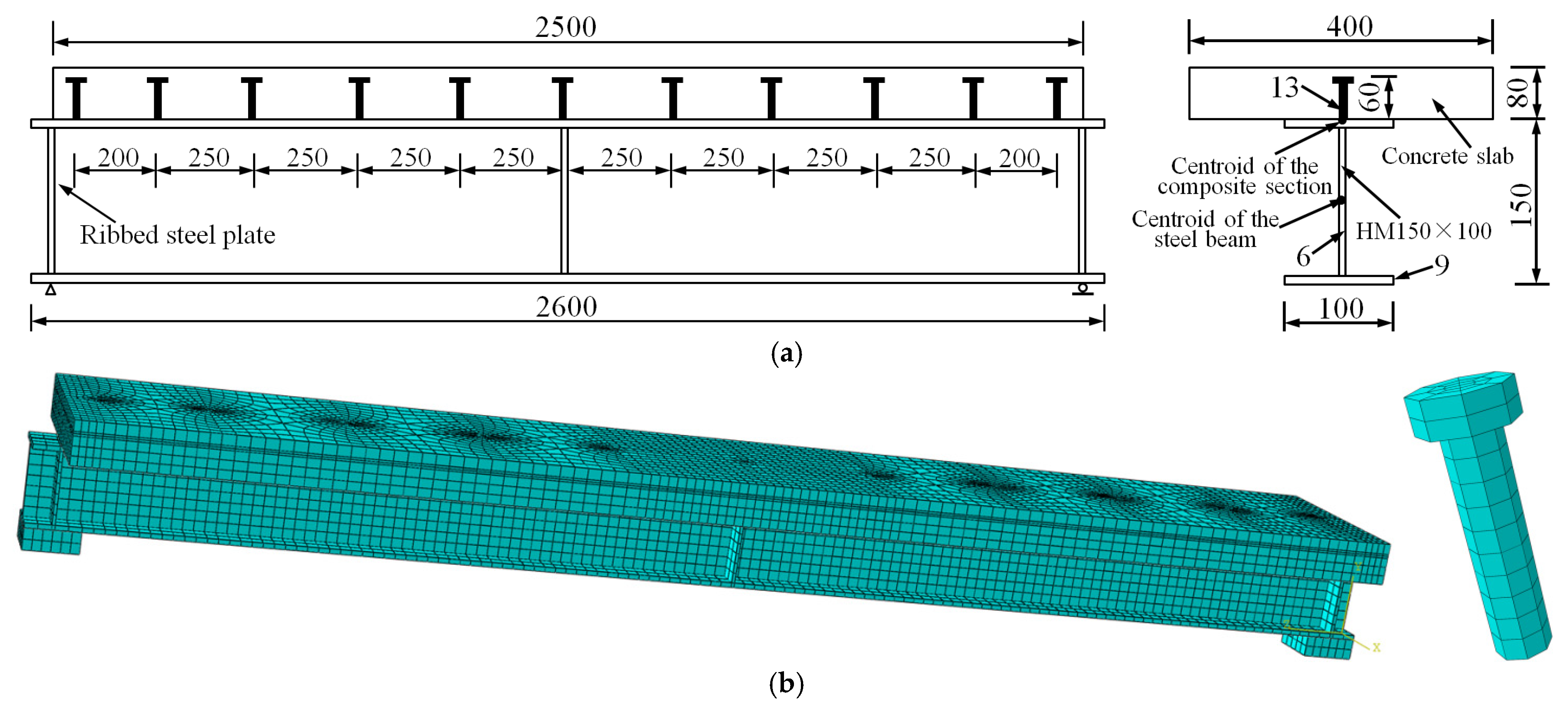
3.3. FE Model Verification 2

The second FE model presented herein refers to the dynamic test conducted by Wang et al. [24] to validate the effectiveness of the proposed modeling methods in modal analysis. The dynamic analysis was performed in the linear perturbation module available in ABAQUS. The test beam was simply supported with a net span of 3800 mm. The ML15 headed studs with a diameter of 13 mm and a height of 60 mm were arranged in double rows along the longitude of the SCCB. The profiled steel HM 200 × 150 was utilized as the steel beam. Detailed dimensions and the distribution of the headed studs in the composite beam are shown in Figure 6a.

Table 2. Material properties of FE model 2.

Material	Yield Strength (MPa)	Ultimate Strength (MPa)	Elastic Modulus (GPa)	Thickness or Diameter (mm)	Density (kg/m3)
Steel beam	437	514	211	9/6	7850
Headed stud	350	467.3	208	13	7850
Concrete	−	53.67	35.13	−	2500
Rebar	270	−	208	6	7850

provides the detailed properties of the materials adopted for the solid-slipping beam model.

Similar to the FE model 1, the normal and tangential behavior between contact surfaces was defined using the “HARD” and “PENALTY” options, respectively. The friction coefficient was set to 0.05 for the interface between the steel flange and concrete slab and 0.45 for the surface of the headed stud and the surrounding concrete by re-running the simulation and comparison. In the linear perturbation module of ABAQUS, the CDP model was disabled; therefore, the constitutive model adopted for concrete was substituted with the linear elastic model. The C3D8R element defined by the tri-linear constitutive model was adopted for the steel beam and headed studs. The three-dimensional truss element (T3D2) was designated for steel reinforcement. The embedding constraint was applied between the reinforcement truss and the concrete slab.

A general mesh size of 50 mm was used for the overall structure, and a fine mesh size of 5 mm was adopted for head studs and the region around head studs. The vertical restraints were applied to both end supports of the SCCB; meanwhile, lateral restraints were applied to the flank side of the beam. Figure 6 provides the first two flexural modal shapes, and

Table 3. Comparison of vibration modes.

Flexural Modes	1	2	3	4	5
FEM frequency (Hz)	33.08	109.20	202.22	351.52	455.50
Test frequency (Hz)	31.25	102.52	201.37	363.09	455.01
Error	5.52%	6.12%	0.42%	3.29%	0.11%

provides a comparison of the natural frequency obtained from experimental and FE analysis. The results compare well; the maximum error was about 6%.

4. Localization of the Damaged Head Studs

In Section 3, the solid-slipping nonlinear FE model for SCCBs was built, and the effectiveness of the FE model was validated from the perspective of mechanical analysis and vibration analysis. In this section, the modal shape and corresponding natural frequency are extracted from the ABAQUS output database to calculate the two vibration-based indicators based on Equations (4) and (9) for localizing the damaged shear studs in SCCBs. All calculation scripts were written in MATLAB R2021a software.

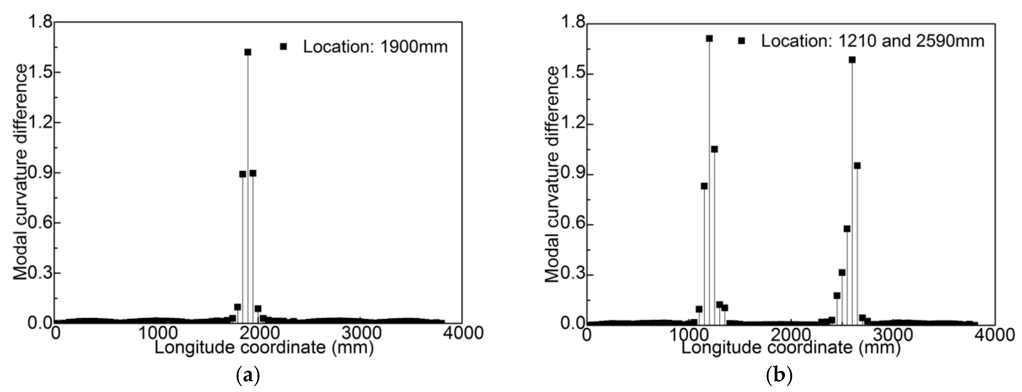
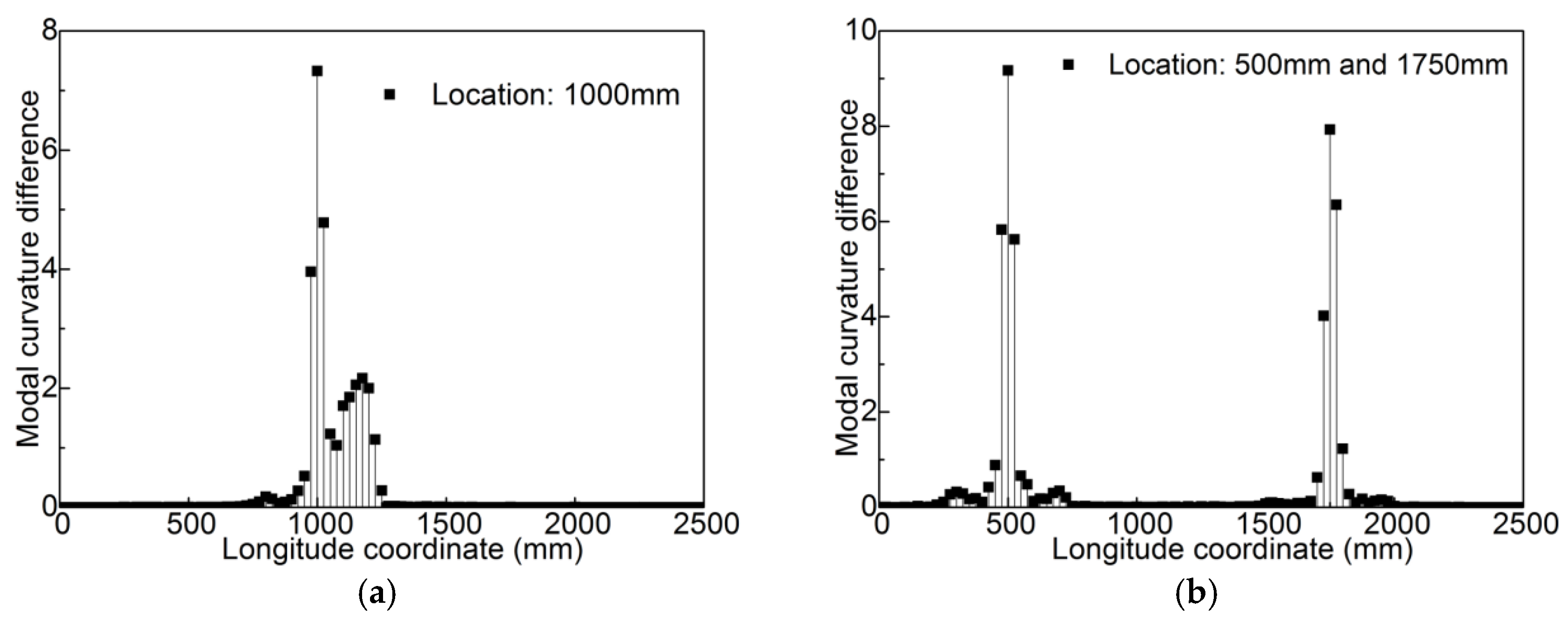
4.1. Damage Localization Based on Modal Curvature Difference

(1) Case 1

Case 1 refers to the validated FE model in Section 3.3, where the damage was simulated by deleting the headed shear studs at corresponding coordinate positions. The first three modal shapes were used to calculate the modal curvature difference. Figure 7 provides the calculated modal curvature difference distributed along the longitude of the SCCB. The damaged shear studs are located at 1900 mm for Figure 7a and 1210 and 2590 mm for Figure 7b. According to Figure 7, the calculated modal curvature difference manifests the damaged shear studs effectively, for both sole-damage and dual-damage conditions. The maximum error was no more than 1%.

(2) Case 2

To guarantee the validity of the proposed flexibility difference curvature for damage location, another steel–concrete composite beam was modeled in ABAQUS. The design of the composite beam was based on the Euler–Bernoulli beam theory and in compliance with the provisions in the Chinese Code for design of steel structure (GB 50017-2017) [25] and the Chinese technical specification for steel structure of tall building (JGJ 99-2015) [26]. Details of the composite beam are described below:

The simply supported composite beam was designed with a partial shear connection of 65%, a net span of 2500 mm, and a total height of 230 mm. The ML15 headed stud has a diameter of 13 mm and a height of 60 mm. The concrete slab has a cross section of 400 × 80 mm. The profiled steel HM 150 × 100 was utilized as the steel beam. Detailed dimensions and the distribution of headed studs are shown in Figure 8a.

Figure 8b provides overviews of the three-dimensional FE model considering the actual geometry, material non-linearity, and boundary constraints. The friction coefficient was assumed to be 0.05 for the interface between the steel flange and concrete slab, and 0.45 for the surfaces of the shear studs and surrounding concrete. A general mesh size of 20 mm was adopted for the overall structure, and a fine mesh size of 5 mm was adopted for head studs and surrounding concrete, as shown in Figure 8b. The constitutive model of all materials was consistent with Section 3.3.

Table 4. Material properties of Case 2.

Material	Yield Strength (MPa)	Ultimate Strength (MPa)	Elastic Modulus (GPa)	Thickness or Diameter (mm)	Density (kg/m3)
Steel beam	205	300	206	9/6	7850
Headed stud	320	400	206	13	7850
Concrete	−	26.8(C40)	31.1	−	2450

provides the detailed properties of the materials. The linear perturbation analysis and Lanczos iteration were adopted to obtain the flexural modal shapes and corresponding natural frequencies.

In Case 2, the damage was also simulated by deleting the headed shear studs at corresponding coordinate positions. The modal curvature differences were calculated based on the first three flexural modal shapes. Figure 9 shows that the distribution of the modal curvature difference manifested the location of damaged studs for both sole-damage and dual-damage conditions successfully.

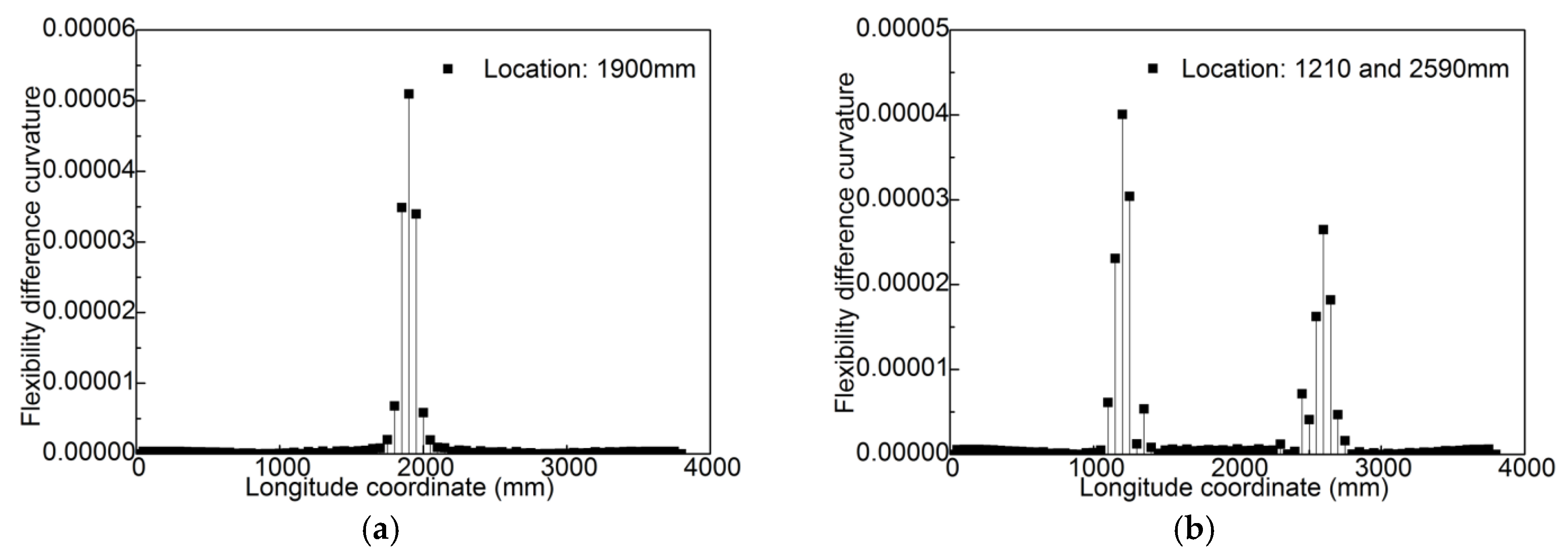
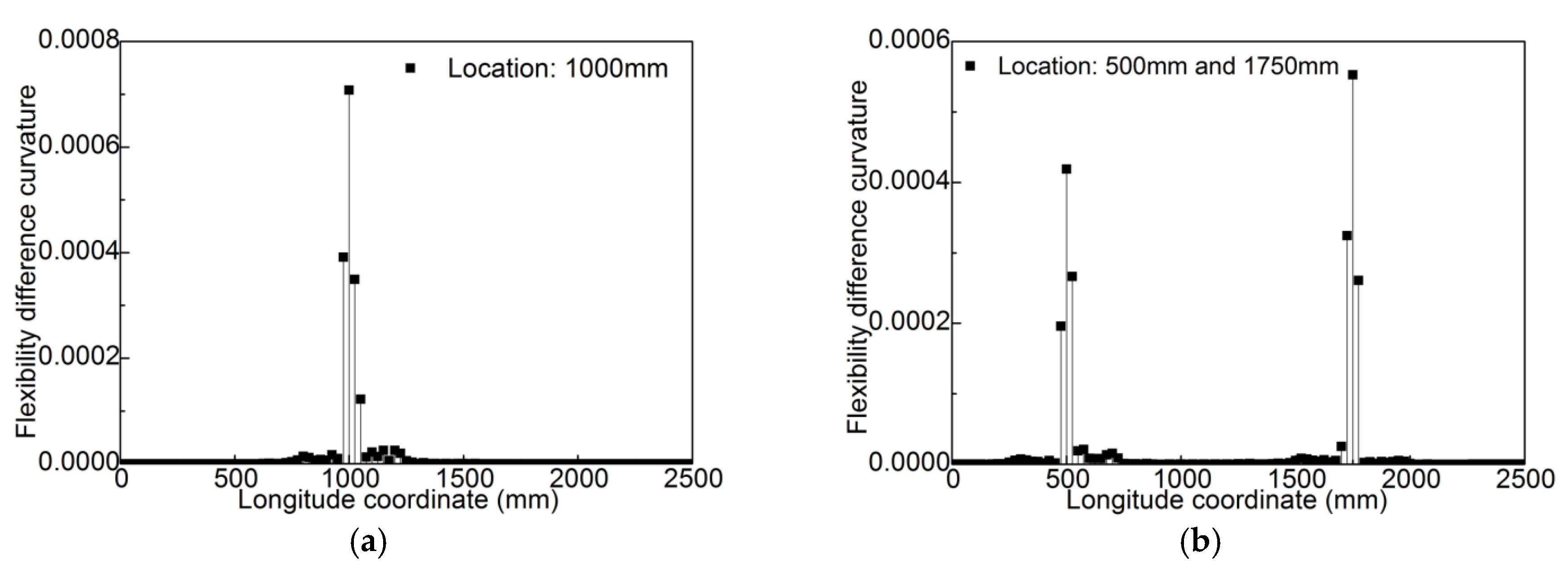
4.2. Damage Localization Based on Modal Flexibility Difference Curvature

Figure 10 and Figure 11 provide the localization results of different damage conditions for Cases 1 and 2, respectively. Similar to the results based on modal curvature difference, all damaged shear studs in SCCB were determined effectively by the calculated modal flexibility difference curvature.

5. Quantification of the Damaged Shear Studs

This section reports a quantification analysis to validate the discernibility of the proposed indicators of minor damage to shear studs in SCCBs, where the damage to the shear studs was defined by decreasing the elastic modulus to a certain degree.

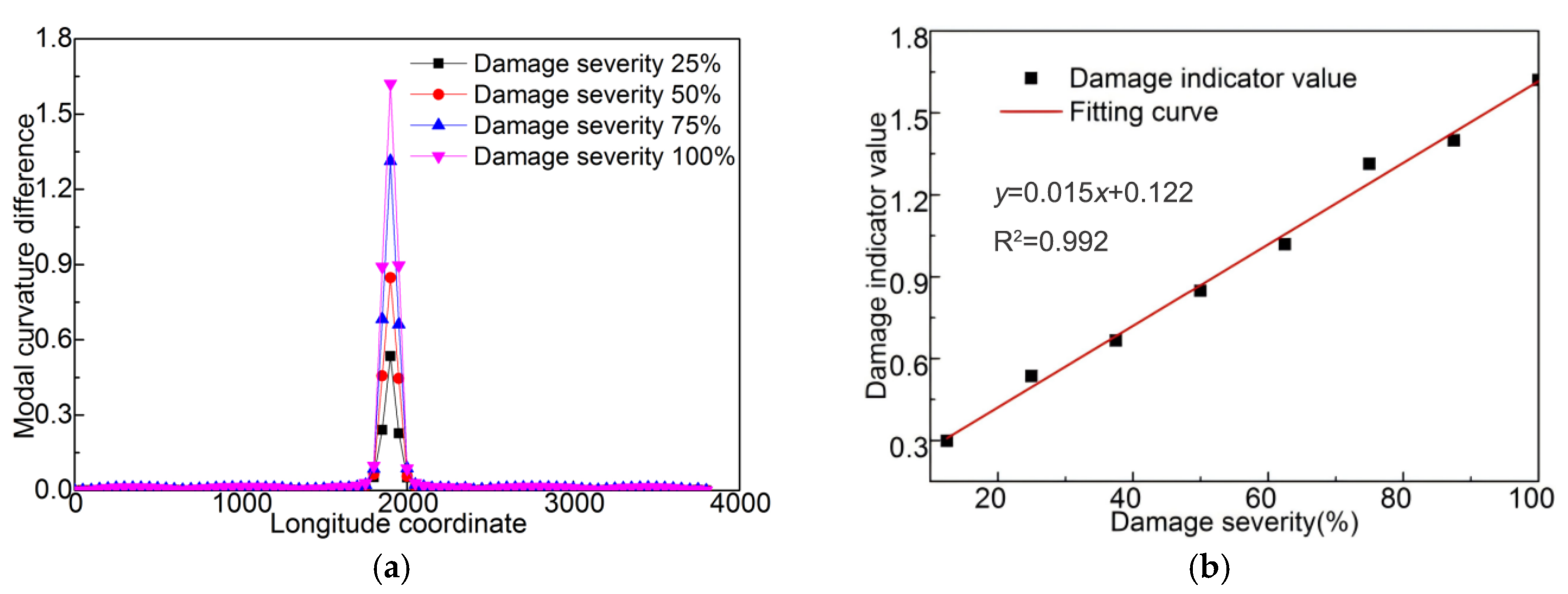
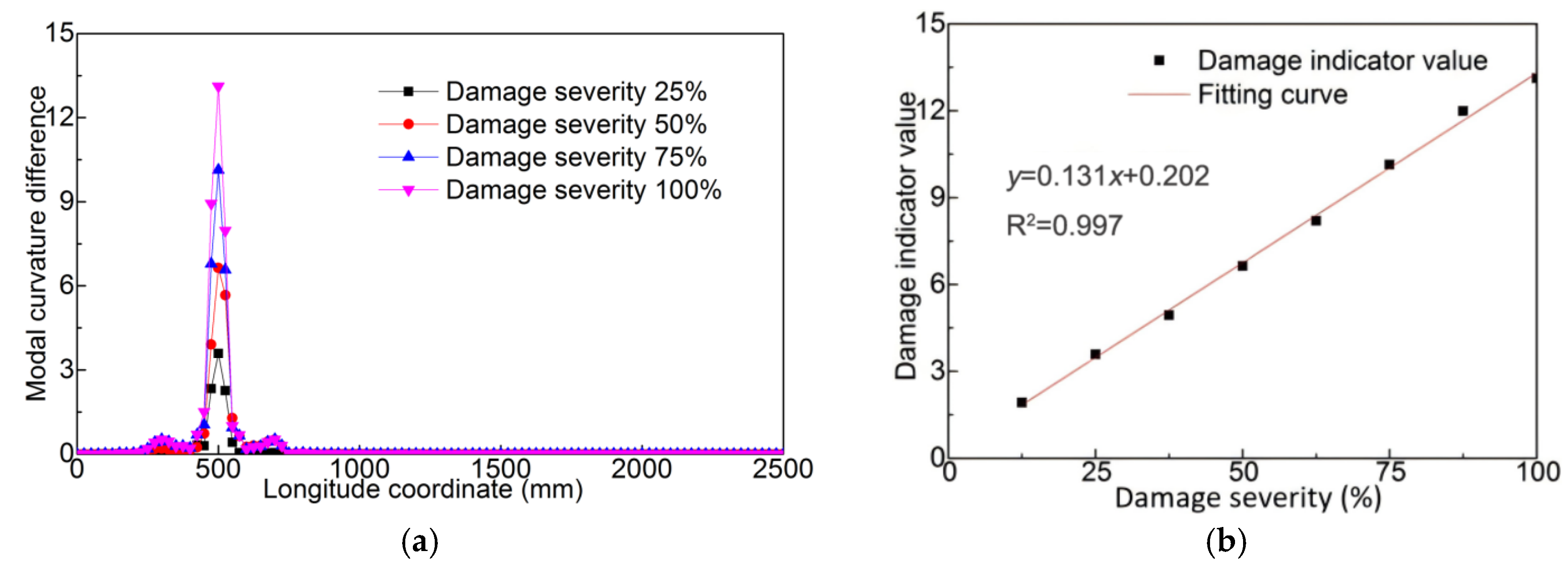
5.1. Damage Quantification Based on Modal Curvature Difference

Figure 12 and Figure 13 provide the quantitative evaluation of the damaged studs based on the modal curvature difference for Case 1 and Case 2, respectively. Figure 12a and Figure 13a show that the calculated modal curvature difference identified the damaged stud when the damage degree was 25% or even lower. According to Figure 12b and Figure 13b, the damage index showed a good linear relationship with the increase in damage degree (R² ≥ 0.992). Thus, the proposed modal curvature difference can be regarded as a favorable indicator to quantify the damage degree of the shear studs in SCCBs and provide guidance for structural rehabilitation.

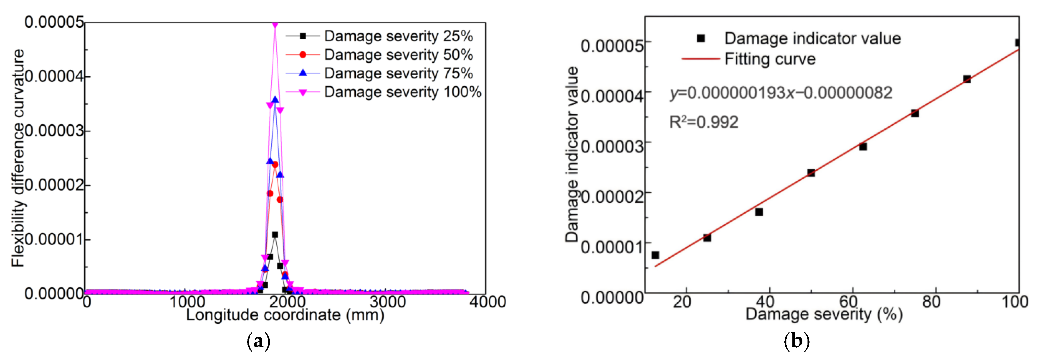
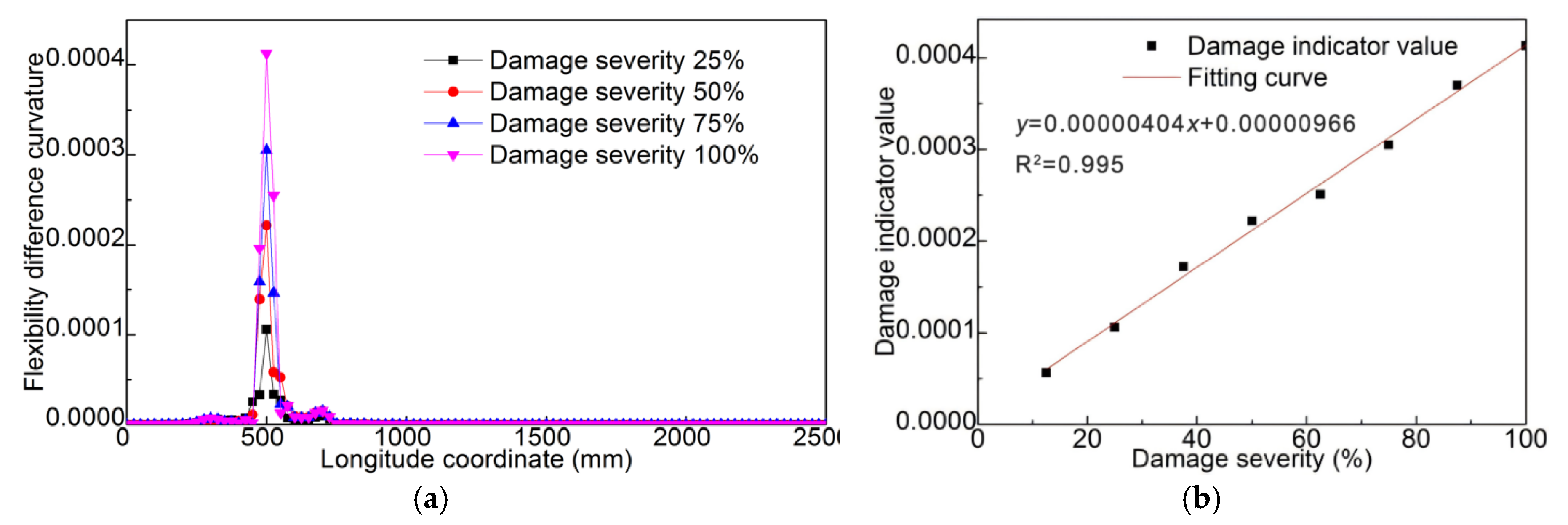
5.2. Damage Quantification Based on Modal Flexibility Difference Curvature

Figure 14 and Figure 15 provide the quantitative evaluation of the damaged studs based on the modal flexibility difference curvature for Cases 1 and 2, respectively. Similar to the results of modal curvature difference (Section 5.1), the proposed modal flexibility difference curvature provided quantitative information for the damaged studs. The linear relationship in Figure 14b and Figure 15b also proved the modal flexibility difference curvature to be a good indicator to quantify and prognose the damages of shear studs in steel–concrete composite beams.

6. Robust Analysis

Attractive features of curvature-based indicators include high sensitivity to damage, and the instant determination of the damage location has been proven. However, the effect of ambient noises and errors in modal shape information will weaken the accuracy and efficiency of the curvature-based indicators. Therefore, this section conducts a thorough, robust analysis to validate the practicability of curvature-based indicators under ambient noises and to complement modal shape information. The modal curvature difference and modal flexibility difference curvature are calculated based on Equations (4) and (9), respectively.

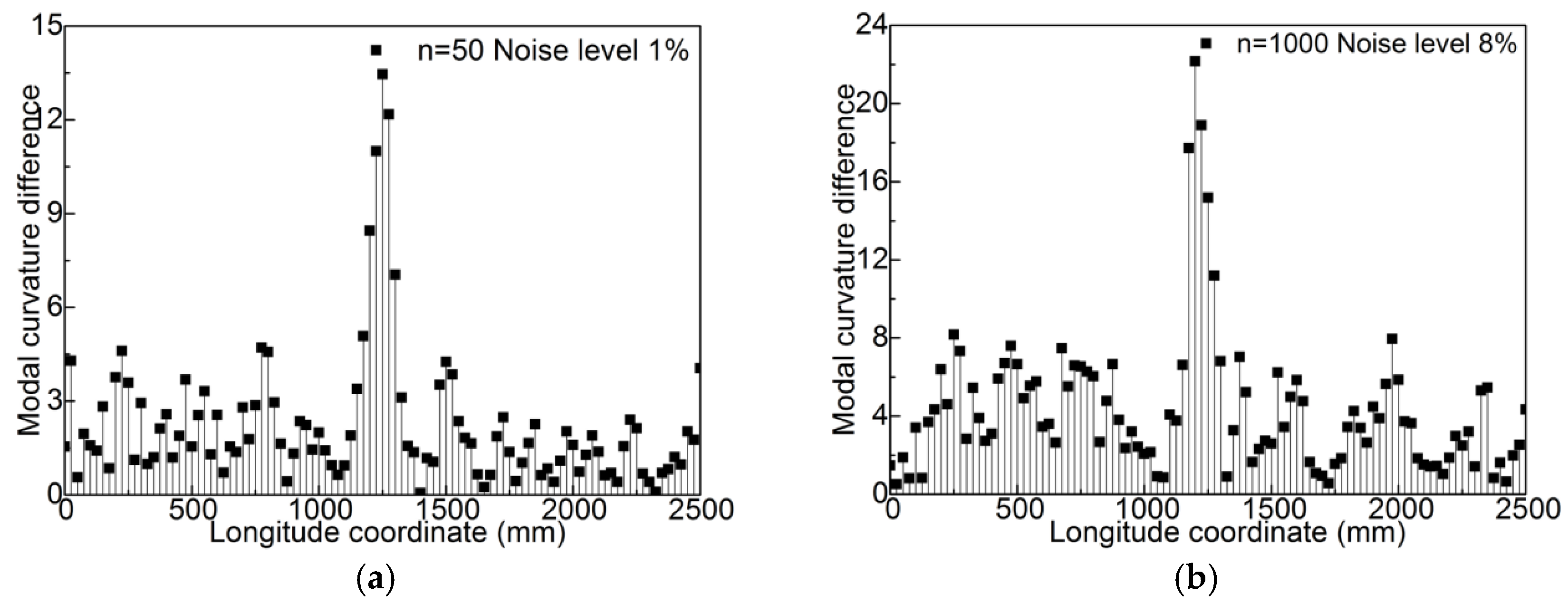
6.1. The Influence of Ambient Noises

The Gaussian white noise was added to the obtained modal shapes as in Equation (12):

$${\phi }_{ij}^{\prime }={\phi }_{ij}\left(1+rand()\cdot \epsilon \cdot {\phi }_{\max ,j}\right)$$

(12)

where ${\phi }_{ij}^{\prime }$ is the modal displacement of the jth point of the ith modal shape with noise, φ_ij is the corresponding modal displacement without noise; ε is the noise level; and rand() represents the random standard normal distribution.

To weaken the influence of noise, each ${\phi }_{ij}^{\prime }$ was decomposed and reconstructed by wavelet transform and averaged n times. Figure 16 and Figure 17 show the influence of ambient noise on the modal curvature difference and the modal flexibility difference curvature; the shear stud was damaged at the mid-span of the SCCB (1250 mm). Figure 16a and Figure 17a indicate that the two calculated indicators located the damaged studs successfully when the noise level was 1% and 0.6%, respectively. With the increase in the average times n, the robustness to ambient noises also increased. Figure 16b and Figure 17b show that when the average times n = 1000, the corresponding noise level can be up to 8% and 5% for the modal curvature difference and the modal flexibility difference curvature, respectively. By comparison, the proposed modal curvature difference showed a better robustness to ambient noises than the modal flexibility difference curvature.

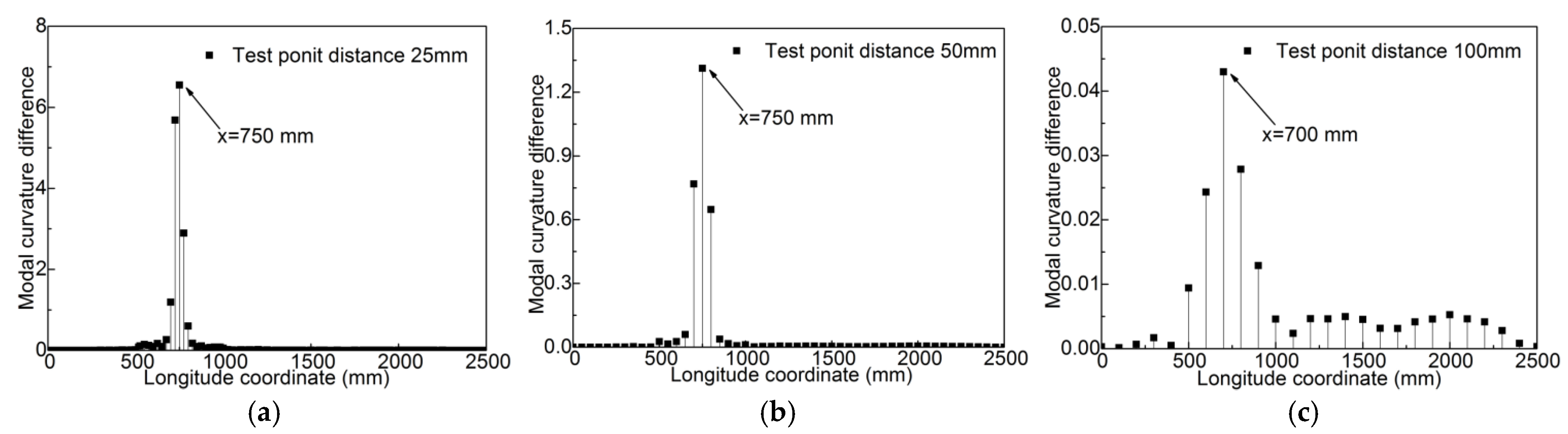
6.2. The Influence of Incomplete Modal Information

Figure 18 and Figure 19 show the influence of incomplete modal information on the two proposed indicators for the damaged shear stud located at 750 mm. One can see that with the test point distance increasing from 25 mm to 100 mm (measurement points decreased 75%), the proposed indicators identified the damaged studs with a maximum error of 50 mm, as shown in Figure 18c and Figure 19c. Considering the fact that the distance between two shear studs was 250 mm, the error does not have much influence on the determination of damage location. Prospectively, the measurement points can be further decreased, but the corresponding test error will increase.

7. Conclusions

This study reported on the damage localization and quantification for the shear studs in steel–concrete composite beams (SCCB) by two novel proposed indicators. Conclusions are drawn as follows:

(1)

A solid-slipping nonlinear finite element (FE) model for SCCBs was developed with the supercities of high precision and independent of stiffness-slip function.

(2)

Two indicators based on the vibration curvature of SCCB were proposed, which are able to locate the damaged shear studs and quantify the damage degree for both sole damage and multi-damage, having a maximum error of no more than 1%.

(3)

Robust analysis proved that the proposed indicators worked well, even though the ambient noise was up to 8% and measurement points decreased by 75%, and the proposed modal curvature difference showed a better robustness to ambient noises than the modal flexibility difference curvature.

However, the results were based on limited numerical analysis; further experimental and in situ studies are needed to promote the practical application of the proposed methods.

References

1. Henderson, I.E.J.; Zhu, X.Q.; Uy, B.; Mirza, O. Dynamic Behaviour of Steel-concrete Composite Beams Retrofitted with Various Bolted Shear Connectors. Eng. Struct. 2017, 131, 115–135. [Google Scholar] [CrossRef]
2. Lima, J.M.; Berzrrra, L.M.; Bonilla, J.; Mirambell, E. Experimental Study on Full Scale Steel-concrete Composite Beams Using Truss-type Shear Connectors. Eng. Struct. 2024, 303, 117490. [Google Scholar] [CrossRef]
3. Dilena, M.; Morassi, A. Vibrations of Steel-Concrete Composite Beams with Partially Degraded Connection and Applications to Damage Detection. J. Sound Vib. 2009, 320, 101–124. [Google Scholar] [CrossRef]
4. Hou, Z.M.; Xia, H.; Zhang, Y.L. Dynamic Analysis and Shear Connector Damage Identification of Steel-concrete Composite Beams. Steel Compos. Struct. 2012, 13, 327–341. [Google Scholar] [CrossRef]
5. Gu, Y.; Lu, Y. Stiffness Characteristics of Composite Beams and Application in Damage Identification. J. Eng. Mech. 2024, 149, 04023063. [Google Scholar] [CrossRef]
6. Cuadrado, M.; Jesús, P.S.; José, A.A.G.; Varas, D. Detection of Barely Visible Multi-impact Damage on Carbon/Epoxy Composite Plates Using Frequency Response Function Correlation Analysis. Measurement 2022, 196, 111–194. [Google Scholar] [CrossRef]
7. Dilena, M.; Morassi, A. Experimental Modal Analysis of Steel Concrete Composite Beams with Partially Damaged Connection. J. Vib. Control 2004, 10, 897–913. [Google Scholar] [CrossRef]
8. Chellini, G.; De Roeck, G.; Nardini, L.; Salvatore, W. Damage Analysis of a Steel-concrete Composite Frame by Finite Element Model Updating. J. Constr. Steel Res. 2010, 66, 398–411. [Google Scholar] [CrossRef]
9. Brigante, D.; Rainieri, C.; Fabbrocino, G. The Role of the Modal Assurance Criterion in the Interpretation and Validation of Models for Seismic Analysis of Architectural Complexes. Procedia Eng. 2017, 199, 3404–3409. [Google Scholar] [CrossRef]
10. Gohar, S.; Matsumoto, Y.; Maki, T.; Sakuma, S. Investigation into Vibration—Based Structural Damage Identification and Amplitude—Dependent Damping Ratio of Reinforced Concrete Bridge Deck Slab under Different Loading States. J. Civ. Struct. Health 2023, 13, 133–148. [Google Scholar] [CrossRef]
11. Mehboob, S.; Zaman, Q.U. Vibration-based Method for Story-level Damage Detection of the Reinforced Concrete Structure. Comput. Concr. 2021, 21, 29–39. [Google Scholar]
12. Yin, T.; Jiang, Q.; Yuen, K. Vibration-based Damage Detection for Structural Connections Using Incomplete Modal Data by Bayesian Approach and Model Reduction Technique. Eng. Struct. 2017, 132, 260–277. [Google Scholar] [CrossRef]
13. Xia, Y.; Hao, H.; Deeks, A.J.; Zhu, X. Condition Assessment of Shear Connectors in Slab-girder Ridges Via Vibration Measurements. J. Bridge Eng. 2008, 13, 43–54. [Google Scholar] [CrossRef]
14. Li, J.; Hao, H.; Xia, Y.; Zhu, H. Damage Detection of Shear Connection in Bridge Structures with Transmissibility in Frequency Domain. Int. J. Struct. Stab. Dyn. 2013, 14, 634–640. [Google Scholar]
15. Dimri, A.; Chakraborty, S. Damage Identification of Reinforced Concrete Slabs Using Experimental Modal Testing and Finite Element Model Updating. Structures 2024, 67, 107–123. [Google Scholar] [CrossRef]
16. Li, J.; Hao, H.; Zhu, H.P. Dynamic Assessment of Shear Connectors in Composite Bridges with Ambient Vibration Measurements. Adv. Struct. Eng. 2014, 17, 617–638. [Google Scholar] [CrossRef]
17. Zhang, C.; Lai, S.X.; Wang, H.P. Structural modal parameter recognition and related damage identification methods under environmental excitations: A review. SDHM Struct. Durab. Health Monit. 2025, 19, 25–54. [Google Scholar] [CrossRef]
18. Huang, Y.; Nie, J.G.; Wei-Jian, Y.I. Stiffness of Steel-concrete Composite Frame Beam with Slip Effect. J. Eng. Mech. 2012, 29, 88–92. [Google Scholar] [CrossRef]
19. Liu, X.P.; Bradford, M.A.; Chen, Q.J.; Ban, H.Y. Finite Element Modelling of Steel-concrete Composite Beams with High-strength Friction-grip Bolt Shear Connectors. Finite Elem. Anal. Des. 2016, 180, 54–65. [Google Scholar] [CrossRef]
20. Rong, Y.; Ren, H.L.; Xu, X.Z. An Improved Damage-plasticity Material Model for Concrete Subjected to Dynamic Loading Case Studies in Construction Materials. Case Stud. Constr. Mater. 2023, 19, e02568. [Google Scholar]
21. Qasem, M.; Hasan, M.; Muhamad, R.; Chin, C.L.; Alanazi, N. Generalised Calibration and Optimization of Concrete Damage Plasticity Model for Finite Element Simulation of Cracked Reinforced Concrete Structures. Results Eng. 2025, 25, 103905. [Google Scholar] [CrossRef]
22. Nguyen, H.T.; Kim, S.E. Finite Element Modeling of Push-out Tests for Large Stud Shear Connectors. J. Constr. Steel Res. 2009, 65, 1909–1920. [Google Scholar] [CrossRef]
23. Lee, P.G.; Shim, C.S.; Chang, S.P. Static and Fatigue Behavior of Large Stud Shear Connectors for Steel–concrete Composite Bridges. J. Constr. Steel Res. 2005, 61, 1270–1285. [Google Scholar] [CrossRef]
24. Wang, J.; Yin, H.; Zhang, S.; Yan, L.; Shuai, L.I. Experimental Investigation on Dynamic Properties of Steel-concrete Composite Beams Considering Effect of Interfacial Slip. J. Bridge Eng. 2016, 37, 142–149. [Google Scholar]
25. GB 50017-2017; Standard for Design of Steel Structures. China Architecture & Building Press: Beijing, China, 2017.
26. JGJ 99-2015; Technical Specification for Steel Structure of Tall Building. China Architecture & Building Press: Beijing, China, 2015.
Figure 1. Shear connection in steel–concrete composite beam: (a) welded shear studs; and (b) perforated plate.
Applsci 15 07313 g001
Figure 2. Force and deformation at the interface between profiled steel and concrete slab: (a) force balance; (b) deformation coordination.
Applsci 15 07313 g002
Figure 3. Stress–strain relationship for the materials: (a) concrete; (b) headed stud and structural steel.
Applsci 15 07313 g003
Figure 4. Schematic and FE model of composite beams: (a) schematic of composite beams; (b) FE model of composite beams; and (c) boundary conditions and loading application.
Applsci 15 07313 g004
Figure 5. FEM results of composite beam: (a) load vs. mid-span displacement; and (b) load vs. interface slip.
Applsci 15 07313 g005
Figure 6. Schematic and vibration modal shapes of the composite beams: (a) schematic of composite beams; (b) 1st flexural modal shapes; and (c) 2nd flexural modal shapes.
Applsci 15 07313 g006
Figure 7. Damage localization based on modal curvature difference in Case 1: (a) damage located at 1900 mm; and (b) damage located at 1210 mm and 2590 mm.
Applsci 15 07313 g007
Figure 8. Design and FE model of SCCB (dimension in mm): (a) design drawing; and (b) FE model.
Applsci 15 07313 g008
Figure 9. Damage localization based on modal curvature difference in Case 2: (a) damage located at 1000 mm; and (b) damage located at 500 mm and 1750 mm.
Applsci 15 07313 g009
Figure 10. Damage localization based on modal flexibility difference curvature in Case 1: (a) damage located at 1900 mm; and (b) damage located at 1210 mm and 2590 mm.
Applsci 15 07313 g010
Figure 11. Damage localization based on modal flexibility difference curvature in Case 2: (a) damage located at 1000 mm; and (b) damage located at 500 mm and 1750 mm.
Applsci 15 07313 g011
Figure 12. Quantitative evaluation by modal curvature difference in Case 1: (a) quantitative damage evaluation; and (b) linear fitting of damage indicators.
Applsci 15 07313 g012
Figure 13. Quantitative evaluation by modal curvature difference in Case 2: (a) quantitative damage evaluation; and (b) linear fitting of damage indicators.
Applsci 15 07313 g013
Figure 14. Quantitative evaluation by modal flexibility difference curvature in Case 1: (a) quantitative damage evaluation; and (b) linear fitting of damage indicators.
Applsci 15 07313 g014
Figure 15. Quantitative evaluation by modal flexibility difference curvature in Case 2: (a) quantitative damage evaluation; and (b) linear fitting of damage indicators.
Applsci 15 07313 g015
Figure 16. The influence of ambient noises on modal curvature difference in Case 2: (a) n = 50 and noise level = 1%; and (b) n = 1000 and noise level = 8%.
Applsci 15 07313 g016
Figure 17. The influence of ambient noises on modal flexibility difference curvature in Case 2: (a) n = 50 and noise level = 0.6%; and (b) n = 1000 and noise level = 5%.
Applsci 15 07313 g017
Figure 18. The influence of incomplete modal information on modal curvature difference in Case 2: (a) test point distance 25 mm; (b) test point distance 50 mm; and (c) test point distance 100 mm.
Applsci 15 07313 g018
Figure 19. The influence of incomplete modal information on modal flexibility difference curvature in Case 2: (a) test point distance 25 mm; (b) test point distance 50 mm; and (c) test point distance 100 mm.
Applsci 15 07313 g019