Analysis of High-Power Radar Propagation Environments Around the Test Site

Abstract

In this paper, we propose a novel evaluation method to assess the strength of electromagnetic (EM) waves in a specific area by analyzing the propagation environment at a radar testing site. To analyze the propagation environment of the radar test site, this evaluation method performs precise modeling of actual structures such as buildings and terrain. The calculated received power is then converted into electric field strength to compare with the reference threshold level (61 V/m). The electric field during the radar operation is examined by changing two scenarios: one is when the transmitter (Tx.) is directed toward the receiver (Rx.), and the other is when the Tx. is misaligned. In particular, it may increase the electric field strength near the Tx. system when Tx. and Rx. are misaligned. To reduce the impact of EM waves, we conducted a comparison based on the installation of absorbers. The results indicate that the received electric field shows attenuation rates of 39.47% in the X-band and 39.35% in the Ku-band, achieved with a 1 m absorber. In addition, the theoretical and average measured received powers of −61.9 dBm and −62.03 dBm, respectively, show good agreement with the simulated result of −64.64 dBm. This measurement procedure exhibits high accuracy when compared with theoretical and simulation results. These results demonstrate the reliability of the propagation environment analysis using the proposed integrated simulation model.

1. Introduction

In military applications, the importance of radar systems capable of accurately detecting and tracking enemy attacks in advance is growing [1,2,3,4]. During the operation of these radar systems, the occurrence of false positives or false negatives can result in unnecessary responses [5,6,7]. Consequently, ensuring reliability and accuracy is crucial for the stable operation of the radar system. For this reason, radar performance testing is considered an essential procedure, which is conducted at test sites similar to actual operating environments [8,9]. This performance test is carried out by steering the Tx. radar toward Rx. probe antenna. In this process, a high power of electromagnetic (EM) waves is emitted not only through the radar’s main lobe but also through the side lobes [10]. These EM waves may be transmitted to areas other than the receiver due to the reflection, diffraction, and scattering caused by the complexity of surrounding structures such as trees and buildings [11,12,13]. In particular, the reference level for electric field strength is established at 61 V/m when the EM waves are transmitted to areas accessible to the general public [14]. Thus, a precise analysis of the propagation environment, including both direct and indirect paths, as well as the electric field strength around the test areas, is required before radar performance testing. To predict such a propagation environment, empirical statistical models such as the Okumura and Hata models, as well as ITU-R models (P.452-17, P.530-18, P.1546-6), which can be applied to various frequencies, have been utilized [15,16,17,18]. However, these models are limited in accuracy because they depend on statistical methods and do not accurately account for structures such as terrain and buildings. Although studies have been conducted in specific regions using precise modeling and simulation (M&S), these have primarily focused on analyzing direct and indirect paths [19,20]. Therefore, comprehensive research is needed to evaluate the impact of environmental factors, including terrain and buildings, on the radio environment surrounding radar test sites.

In this paper, we propose a novel evaluation method for the strength of EM waves in the area by analyzing the propagation environment in a radar testing site. This evaluation method, which utilizes EM simulation, follows three steps: First, to analyze the propagation environment of the radar test site, actual structures, such as buildings and terrain, are precisely modeled. An integrated model is then set up by applying them to a propagation simulation tool (Wireless InSite 3.3.0 software). Herein, the terrain is modeled using digital elevation model (DEM) data provided by the Ministry of Land, Infrastructure, and Transport. Second, the EM waves transmitted from the Tx. system to Rx. system are classified into the direct path and the indirect path. The received power around each system is analyzed based on the sum of these paths. Third, we convert the calculated received power into electric field strength for comparison with a reference threshold level. Through this process, we analyze two scenarios: one is when the Tx. is directed toward the Rx., and the other is when the radar is misaligned. Finally, in the misaligned scenario, we evaluate the electric field strength by placing absorbers on the Tx. radar building. To verify the accuracy of the proposed evaluation method, we conduct measurements at an actual radar site and compare the measured received power with the simulation results.

2. Method for Analyzing Propagation Environments and Modeling Radar Sites

Figure 1 illustrates the propagation environment scenario at the radar performance test site. In this scenario, the Tx. system, located above the radar control center, emits EM waves directed toward the Rx. system, which is placed at the top of a beacon tower at a height of 60 m. Herein, various geographical features, such as buildings, a river, and mountains, are distributed between each system (distance of 850 m). Because of these features, EM waves propagate not only through a direct path but also through indirect paths, which occurs by reflection, diffraction, and scattering. In particular, high electric field strength can be transmitted around the Tx. system through both direct and indirect paths due to reflection or malfunctions of the radar system. The areas that can be reached by indirect paths are classified as important observation areas, and the received EM waves should be considered. To analyze the propagation environment in such specific areas, the ray-tracing method based on geometrical optics (GO) and the Uniform theory of diffraction (UTD) can be utilized. The received power can be represented as the sum of the received power from both direct and indirect ray paths, as expressed in the following equation [21]:

$$P_t(s)=P_d(s_d)+{\displaystyle \sum _{i=1}^N{P}_{g,i}(s_i)}+{\displaystyle \sum _{j=1}^M{P}_{u,j}(s_j)},$$

(1)

where P_t(s) is the total received power at a specific point s, which consists of the P_d(s_d) transmitted through direct paths, the sum of P_g,i(s_i) transmitted through reflected paths, and the sum of P_u,j(s_j) transmitted through diffracted paths. Here, s_d represents the distance of the direct path, while s_i and s_j denote the distances of the i-th reflected path and the j-th diffracted path, respectively. N is also the total number of reflected paths, and M denotes the total number of diffracted paths. The electric field strength is then determined based on the received power to evaluate the impact of the radar on the observation area. The electric field strength can be calculated from the received power using the following equation [22]:

$$E_r=\sqrt{\eta {\displaystyle \frac{P_t\cdot 4\pi }{G_r{\lambda }^2}}},$$

(2)

where η is the intrinsic impedance (Ω) in free space, P_t is the received power (W), G_r is the gain of the receiving antenna, and λ is the wavelength. Since this value varies depending on the input power and frequency of the radar, accurate analysis enables the assessment of the impact of received EM waves on the radar site.

Figure 2 represents the simulation model for analyzing the propagation environment during the test of radar performance. In this study, we employ Wireless InSite by Remcom, which utilizes the ray-tracing method to analyze the propagation environment [23]. For accurately analyzing propagation characteristics such as reflection, diffraction, and scattering, this simulation model consists of three parts: terrain, buildings, and a river. First, to apply complex terrain into the simulation, we utilize DEM data provided by the Ministry of Land, Infrastructure, and Transport [24]. This data has a higher resolution (1 m) compared to the NASA and Google terrain data (20–30 m) used in previous studies, allowing for a more effective simulation of complex terrain features [25]. Structures such as buildings and river are then modeled on the terrain. Herein, the material characteristics of structures are applied separately. The DEM terrain data is modeled as wet earth (ε_r = 20, σ = 0.02 S/m), and the material properties of building structures are set as concrete (ε_r = 15, σ = 0.015 S/m). The water of the river is also modeled as fresh water (ε_r = 81, σ = 0.22 S/m). The number of ray paths arriving at each receiver is limited to a maximum of 25, and each ray carried a sinusoidal signal with a bandwidth of 1 MHz. The ray-tracing simulation is configured in narrowband mode at the operating frequency, enabling accurate comparison with the measurement and theoretical results.

3. Analysis of the Propagation Environment During Radar Operation

Figure 3 illustrates the radiation patterns of the radar system used in the simulation. In our study, we analyze the X-band and Ku-band frequencies based on actual radar specifications. The beam pattern for the patch array antenna is generated using the antenna design software CST Studio Suite 2020 EM simulator [26] and then converted into a format compatible with Wireless InSite. The radiation patterns of the radar system are generated using a uniform planar array of single patch antennas, based on the standard array factor approach. In Figure 3a, the red solid line indicates the radiation pattern for the X-band, while the blue line presents the radiation pattern for the Ku-band. The generated X-band radar radiation pattern has a bore-sight gain of 30.07 dBi, a 3 dB beamwidth of 4.9°, and a sidelobe level of 13.3 dB. The Ku-band radiation pattern has a bore-sight gain of 35.86 dBi, a 3 dB beamwidth of 2.2°, and a sidelobe level of 13.5 dB. The characteristics of the X-band and Ku-band radar systems are listed in

Table 1. Characteristics of the radar system radiation patterns.

Parameters	X-Band (8 GHz)	Ku-Band (18 GHz)
Realized gain (dBi)	30.07	35.86
3 dB beam width (°)	4.9	2.2
Side lobe level (dB)	13.3	13.5

. Figure 3b shows 3D radiation pattern of test radar in simulation model. In the simulation, the radiation pattern of the test radar is positioned 5 m above the top of the radar control center, and the frequency-specific radiation patterns shown in Figure 3a are applied according to each simulation case.

Figure 4 illustrates the analysis of the propagation environment in a radar testing scenario using the proposed simulation model. To analyze the EM waves transmitted around the Tx. system and Rx. system through both direct and indirect paths, the observation points are placed at 2 m intervals in the radar site. Herein, the direct path refers to the line-of-sight (LoS) between the Tx. and Rx. of the radar system, while the indirect path consists of waves that are reflected, diffracted, or scattered by terrain and buildings. A λ/4 monopole antenna (5.15 dBi) is placed at the top of the beacon tower (60 m above the ground) to examine the propagation path to the Rx. System. Figure 4a shows not only the direct path (red solid line) but also the indirect path (yellow solid line), which is caused by the side lobe of the radar and reflection by the terrain. Although the radar is directed towards the Rx. system, the results indicate that the transmitted EM waves reach the surrounding terrain and are received through various paths due to reflection and diffraction. Figure 4b provides the received power distribution around the Tx. radar and the Rx. system in the X-band. The transmitted power of the radar is set at 1 W (30 dBm), and the received power at each location is listed in

Table 2. Received power at the analyzed frequency.

		X-Band	Ku-Band
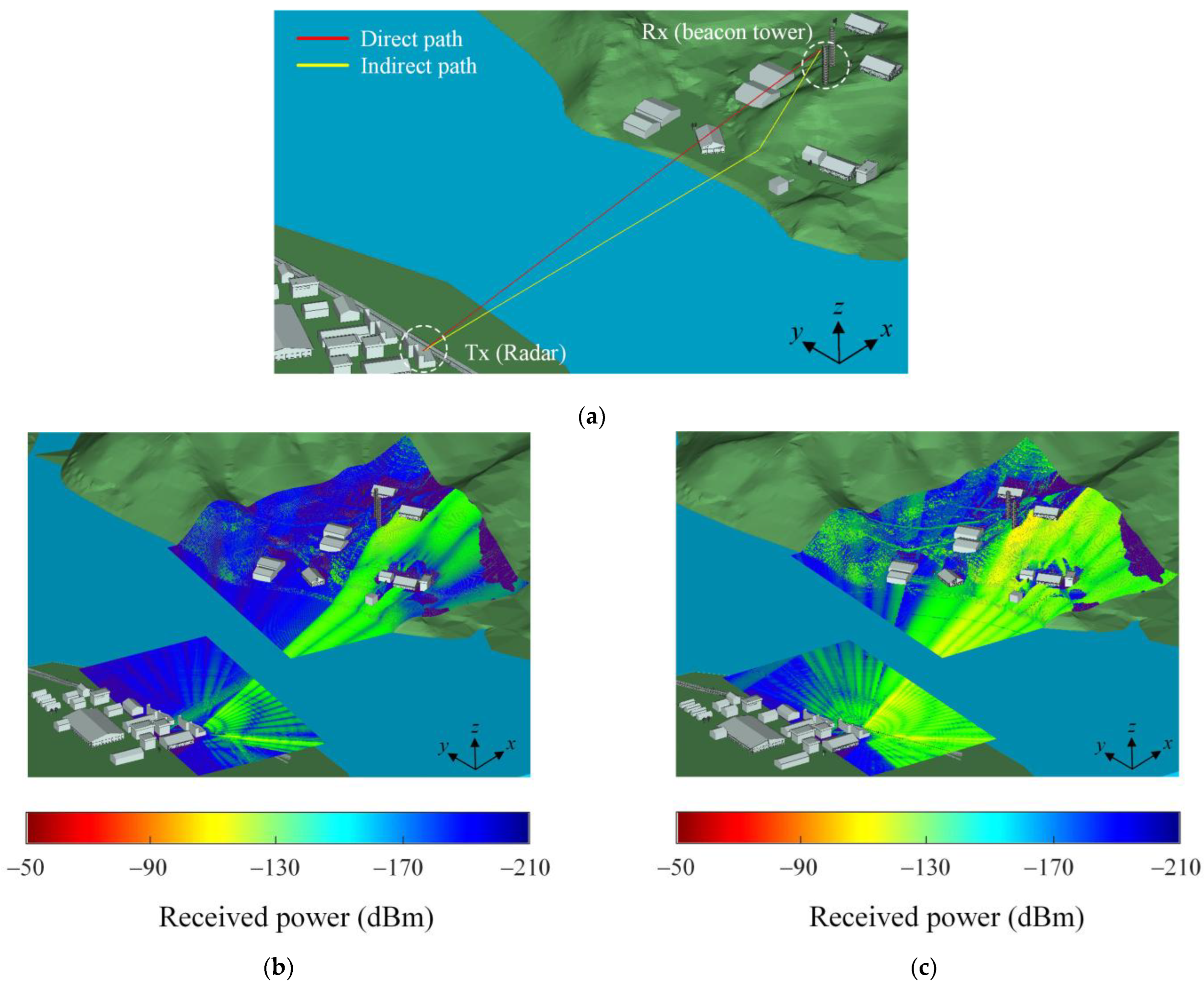
Minimum received power (dBm)	Tx. area	−216.75	−218.17
	Rx. area	−218.87	−219.95
Maximum received power (dBm)	Tx. area	−44.39	−59.09
	Rx. area	−52.86	−59.94

. According to the results of the X-band, the maximum received power of −44.39 dBm and −52.86 dBm in the surrounding areas of the Tx. and Rx. systems are calculated, respectively. These results can be converted to electric field strengths of 0.19 V/m and 0.07 V/m, which are significantly lower than the reference level of 61 V/m. Figure 4c represents an analysis for the Ku-Band, and the maximum received power of −59.09 dBm (0.08 V/m) and −59.94 dBm (0.07 V/m) is calculated and confirmed to be lower than the reference level.

Figure 5 illustrates the distribution of received power in the X-band and Ku-band with steering toward a nearby area. The transmitted power is set to 1 W, and the elevation angle of the radar is adjusted to −30°, which allows the signal to reach the nearby area in the shortest distance. The transmitted power is attenuated by a path loss of 88.2 dB and 96.6 dB in the X-band and Ku-band, respectively, over 76.7 m until reaching the ground. Based on the simulation, the received power is calculated as −26.48 dBm (1.52 V/m) and −28.32 dBm (2.77 V/m) in the X-band and Ku-band, respectively. Although the electric field does not exceed the reference level in either the X-band or Ku-band, the electric field strength around the Rx. system increases compared to the scenario shown in Figure 4. These results show that the proposed method can be used to analyze the potential impact on received EM waves in areas near the radar site in advance, allowing for netter prepare for such situations.

Even though the electric field strength may already be low, the field strength around the radar site can be further minimized in cases where the radar is misaligned. One of the possible solutions is to consider the placement of absorber structures. Figure 6 shows the analysis results of the received power distribution in the nearby area when absorber (ε_r = 22.9 −j1.37, τ = −29.90 dB) structures are placed in front of the Tx. radar. In this analysis, the transmitted power and elevation angle of the Tx. radar systems are set the same as in Figure 5, and absorber structures are placed in front of the radar to analyze the attenuating rate of the received power reaching the nearby area. The height of the absorber is applied from 1 m to 2 m in 0.5 m increments. According to the simulation result with 1 m of absorber height, the received power is calculated as −30.82 dBm in the X-band and −32.67 dBm in the Ku-band at a transmitted power of 1 W, as shown in

Table 3. Maximum received electric field in the analyzed area based on the height of the absorber.

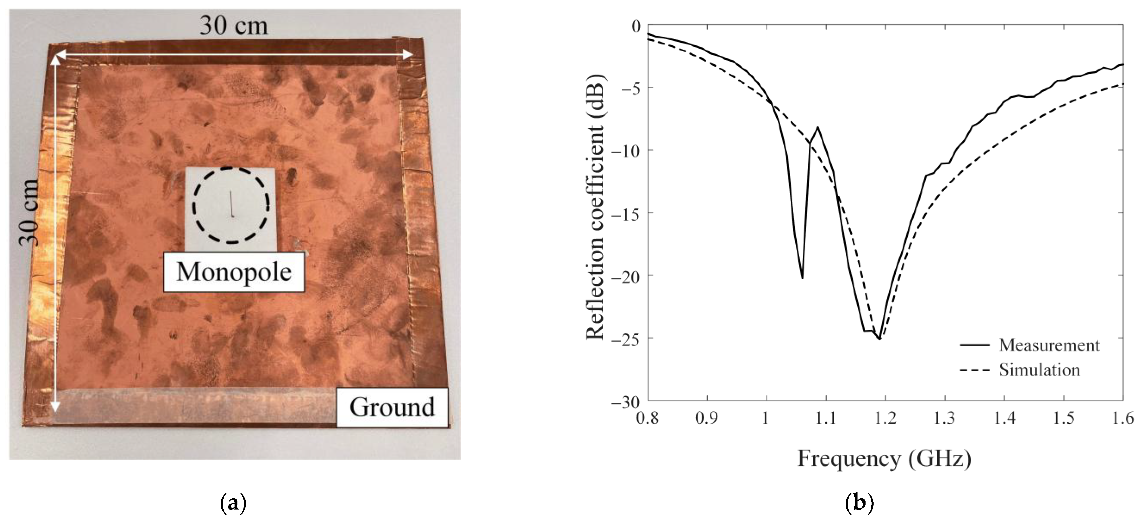
Height of Absorber	Frequency	W/O Absorber	With Absorber	Attenuation Rate
1 m	8 GHz	1.52 V/m	0.92 V/m	39.47%
	18 GHz	2.77 V/m	1.68 V/m	39.35%
1.5 m	8 GHz	1.52 V/m	0.29 V/m	80.92%
	18 GHz	2.77 V/m	0.46 V/m	83.39%
2 m	8 GHz	1.52 V/m	0.17 V/m	88.82%
	18 GHz	2.77 V/m	0.18 V/m	93.5%

. The maximum electric field near the Tx. Radar system is 0.92 V/m for the X-band and 1.68 V/m for Ku-band. A comparison of the received electric field depending on absorber installation shows an attenuation rate of 39.47% and 39.35% in each frequency band. Furthermore, the attenuation rate of the received electric field increases with the height of the absorber structures. In addition, we move the 1 m-high absorber 5 m closer to the radar to assess the impact of its position. In this configuration, the maximum received power is −22.23 dBm, representing an increase of 8.59 dB compared with the original setup. Therefore, installing absorber structures near the Tx. system can further reduce the electric field around the testing areas while the radar system is in operation.

4. Verification of Analysis Results Through Comparison of Measurement and Simulation

To verify the reliability of the results analyzed through the simulation model, measurements are conducted at the actual radar site and compared with the simulation results. This measurement is conducted in the L-band (1.2 GHz) to minimize electromagnetic interference at the operational radar site. The Tx. signal is radiated with a 0 dBm L-band frequency by the signal generator. The Rx. system employs the same monopole antenna as that of the Tx. system and is connected to a spectrum analyzer (Anritsu MS2720T (Anritsu Corporation, Atsugi, Japan)) located approximately 120 m from the Radar Control Center, as shown in Figure 7a. In this simulation setup, the Tx. antenna uses the same monopole antenna as that of the measurement system and is placed in front of the Radar Control Center, with a transmitted power set to 0 dBm. Figure 7b illustrates the measurement setup used to determine the insertion loss of the RF cable for measurement verification. In this setup, a Rohde & Schwarz SMBV100A Vector Signal Generator (Rohde & Schwarz GmbH & Co. KG, Munich, Germany) is configured to output a signal at a frequency of 1.2 GHz with an output power of 0 dBm. This signal is transmitted through the testing RF cable and received by an Anritsu MS2720T Spectrum Analyzer (Anritsu Corporation, Atsugi, Japan), which measures the power level of the received signal. The insertion loss is obtained by subtracting the measured power from the transmitted power (0 dBm). As shown in Figure 7b, the received signal strength at the center frequency of 1.2 GHz is observed to be −5.01 dBm, resulting in a total insertion loss of 5.01 dB.

Figure 8 presents the fabrication and reflection coefficient of the λ/4 monopole antenna used for measurement. Figure 8a provides a fabricated antenna with a radiator placed at the center of a ground plane (30 cm × 30 cm). The radiator of the monopole antenna is designed to operate in the L-band with a length of approximately 6.25 cm. Figure 8b shows the reflection coefficient of the fabricated antenna. The measurement and simulation results are indicated by solid and dashed lines, respectively. The measured reflection coefficient is −25.1 dB, while the simulated result is −24.07 dB at the operating frequency of 1.2 GHz. It is observed that there is a discrepancy between the measured and simulated results, and it can be attributed to parasitic conductance or inductance caused by the discontinuity between the radiator and connector.

Figure 9 represents the radiation patterns of the Tx. and Rx. antenna. The λ/4 monopole antenna is measured in the full anechoic chamber, as shown in Figure 9a. The fabricated antenna is fixed with a Styrofoam jig, and the antenna gains of the fabricated antenna are measured to verify antenna feasibility. Figure 9b,c illustrate the measured and simulated 2D radiation patterns of the monopole antenna (the azimuth and elevation directions). The measured radiation patterns show an omnidirectional pattern with an average gain of 0 dBi, and they also have a good agreement with the simulated result (dashed line).

Figure 10 represents the measurement setup at the actual radar site for verifying the integrated simulation model. In order to verify the free-space loss obtained from simulation, the measured received power is applied into the Friis transmission equation, which includes not only free space propagation loss but also various system level losses, as expressed in the following equation:

$$P_r(dB)=P_t+G_t+G_r-L_{tc}-L_{rc}-L_s-L_p$$

(3)

where P_r is the received power of Rx. antenna (dBm), P_t is the transmitted power of Tx. antenna (dBm), G_t and G_r are the antenna gains at the Tx. and Rx. antenna (dBi), and L_tc and L_rc represent the cable losses (dB), which are integrated with the Tx. and Rx. antenna systems, respectively. L_s also represents other system losses (such as connectors and circuit loss), and L_p is the Free Space Path Loss (FSPL), which depends on the distance between Tx. and Rx. systems, as well as the operation frequency. Since the conventional Friis model assumes ideal transmission conditions, it is necessary to consider the measured cable loss into the equation to reflect the actual signal attenuation in the measurement setup. Radiated power was measured at nine points arranged in a 3 × 3 matrix with 1 m increments. The measured values are listed in

Table 4. Measurement results for analysis verification (dBm).

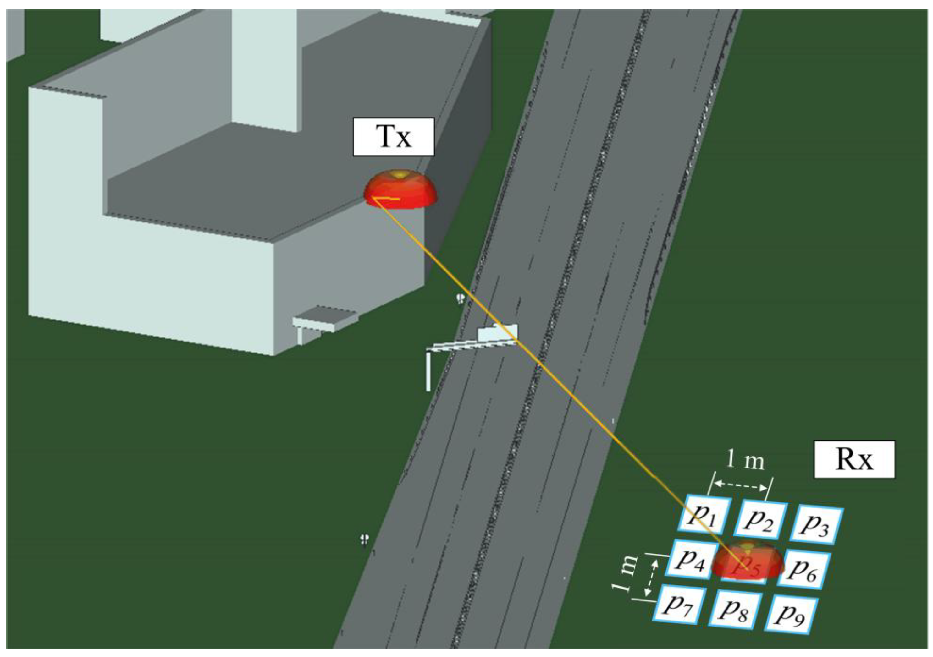
Position	x1	x2	x3
y1	−61.02 (p1)	−61.58 (p2)	−62.41 (p3)
y2	−63.08 (p4)	−59.12 (p5)	−62.32 (p6)
y3	−60.17 (p7)	−62.44 (p8)	−66.12 (p9)

. The averaged measured power is then compared with the simulated result. Herein, the measured data is obtained at nine points (p₁ to p₉) at 1 m intervals, as shown in Figure 10. The averaged measured power is then compared with the simulated result. The comparison of the simulation results, conducted under the same conditions as the theoretical and measurement results, is presented in

Table 5. Comparison of measurement and simulation results.

	Measured	Simulated	Theoretical
Distance (m)	120.59	120.66	120.59
Average received power (dBm)	−62.03	−64.64	−61.9

. The theoretical received power is calculated by accounting for the measured monopole antenna gain, cable loss, and system loss, while the measured received power is averaged over the nine measurement points. The theoretical and average measured received powers of −61.9 dBm and −62.03 dBm, respectively, show good agreement with the simulated result of −64.64 dBm. Therefore, we validate our measurement method and support the reliability of the X-band and Ku-band analyses in Chapter 3. This procedure indicates that the proposed method provides comparable results in theory, simulation, and measurement.

5. Conclusions

In this paper, we proposed a novel evaluation method for the strength of EM waves in the area by analyzing the propagation environment in a radar testing site. To analyze the propagation environment of the radar test site, actual terrain was precisely modeled using DEM data provided by the Ministry of Land, Infrastructure, and Transport. For the scenario of steering towards the Rx. system, the maximum electric fields of 0.19 V/m and 0.08 V/m in the X-band and Ku-band were calculated, respectively. In the misaligned scenario, the maximum electric fields of 1.52 V/m and 2.77 V/m in the X-band and Ku-band were calculated, respectively. These results were significantly lower than the reference level of 61 V/m. To more effectively reduce the impact around the radar site in the misaligned scenario, the absorber structures were placed in front of the radar. With the installation of a 1 m absorber, a comparison of the received electric field showed an attenuation rate of 39.47% and 39.35% in each frequency band. To verify the reliability of the results analyzed through the integrated simulation model, measurements were conducted at the actual radar site and compared with the simulation results. The theoretical and average measured received powers of −61.9 dBm and −62.03 dBm, respectively, showed good agreement with the simulated result of −64.64 dBm. This procedure indicated that the proposed method provided comparable results in theory, simulation, and measurement. These results demonstrated the reliability of the propagation environment analysis using the proposed integrated simulation model.

References

- Bang, S.; Kim, H.; Oh, J. Enhancing 2-D Beam Scanning Capability through Extended Transmission Paths in a Liquid Crystal-Based Transmitarray Antenna for mmWave Communications. J. Electromagn. Eng. Sci. 2025, 25, 85–91. [Google Scholar] [CrossRef]
- Yoon, J.H.; Park, Y.; Roh, J.E. Rejection of Surface Clutter in Far Sidelobes for Airborne Radars. J. Electromagn. Eng. Sci. 2024, 24, 467–476. [Google Scholar] [CrossRef]
- Yousaf, J.; Yakoub, S.; Karkanawi, S.; Hassan, T.; Almajali, E.; Zia, H.; Ghazal, M. Through-the-Wall Human Activity Recognition Using Radar Technologies: A Review. IEEE Open J. Antennas Propag. 2024, 5, 1815–1836. [Google Scholar] [CrossRef]
- Park, J.H.; Park, S.C. Complex Range Resolution Model of Point Scatterers in LFM Chirp Pulse Radar. IEEE Trans. Instrum. Meas. 2022, 71, 4506112. [Google Scholar] [CrossRef]
- Kim, B.; Jin, Y.; Bae, J.; Hyun, E. Two-Step Adaptive Target Detection Scheme Using Beam-Steering FMCW Radar Sensors. J. Electromagn. Eng. Sci. 2024, 24, 674–676. [Google Scholar] [CrossRef]
- Zhong, J.; Zhang, K.; Zeng, Q.; Liu, X. A False Alarm Elimination Algorithm of Foreign Objects Debris Detection Based on Duffing Oscillator. IEEE Access 2022, 10, 7588–7598. [Google Scholar] [CrossRef]
- Chen, X.; Su, N.; Huang, Y.; Guan, J. False-Alarm-Controllable Radar Detection for Marine Target Based on Multi Features Fusion via CNNs. IEEE Sens. J. 2021, 21, 9099–9110. [Google Scholar] [CrossRef]
- Zhu, Y.; Li, Y.; Zhang, Q. False-Alarm-Controllable Radar Target Detection by Differentiable Neyman Pearson Criterion for Neural Network. IEEE Trans. Geosci. Remote Sens. 2023, 61, 5108014. [Google Scholar] [CrossRef]
- Braun, N.; Ziemer, F.; Bezuglov, A.; Cysewski, M.; Schymura, G. Sea-Surface Current Features Observed by Doppler Radar. IEEE Trans. Geosci. Remote Sens. 2008, 46, 1125–1133. [Google Scholar] [CrossRef]
- Conte, E.; De Maio, A.; Farina, A. Statistical Tests for Higher Order Analysis of Radar Clutter: Their Application to L-Band Measured Data. IEEE Trans. Aerosp. Electron. Syst. 2005, 41, 205–218. [Google Scholar] [CrossRef]
- Ng, K.H.; Tameh, E.K.; Nix, A.R.A. New Heuristic Geometrical Approach for Finding Non-Coplanar Multiple Edge Diffraction Ray Paths. IEEE Trans. Antennas Propag. 2006, 54, 2669–2672. [Google Scholar] [CrossRef]
- Silva, J.C.; Costa, E. A Ray-Tracing Model for Millimeter-Wave Radio Propagation in Dense-Scatter Outdoor Environments. IEEE Trans. Antennas Propag. 2021, 69, 8618–8624. [Google Scholar] [CrossRef]
- Puggelli, F.; Carluccio, G.; Albani, M.A. Novel Ray Tracing Algorithm for Scenarios Comprising Pre-Ordered Multiple Planar Reflectors, Straight Wedges, and Vertexes. IEEE Trans. Antennas Propag. 2014, 62, 4336–4339. [Google Scholar] [CrossRef]
- Ministry of Science and ICT. Criteria for Protecting the Human Body from Electromagnetic Waves; No. 2017-7; Ministry of Science and ICT: Sejong, Republic of Korea, 2017. [Google Scholar]
- Deme, A.; Dajab, D.; Bajoga, B.; Mu’azu, M.; Choji, D. Hata-Okumura Model Computer Analysis for Path Loss Determination at 900 MHz for Maiduguri, Nigeria. Math. Theory Model. 2013, 3, 1–9. [Google Scholar]
- International Telecommunication Union. Prediction Procedure for the Evaluation of Interference between Stations on the Surface of the Earth at Frequencies Above About 0.1 GHz; Recommendation ITU-R P.452-17; ITU: Geneva, Switzerland, 2021. [Google Scholar]
- International Telecommunication Union. Propagation Data and Prediction Methods Required for the Design of Terrestrial Line-of-Sight Systems; Recommendation ITU-R P.530-18; ITU: Geneva, Switzerland, 2021. [Google Scholar]
- International Telecommunication Union. Method for Point-to-Area Predictions for Terrestrial Services in the Frequency Range 30 MHz to 4,000 MHz; Recommendation ITU-R P.1546-6; ITU: Geneva, Switzerland, 2019. [Google Scholar]
- Jang, D.; Wang, S.; Kim, C.W.; Park, Y.B.; Choo, H. Method for Estimating Optimal Position of S-Band Relay Station through Path Loss Analysis in an Outdoor Environment. Appl. Sci. 2020, 10, 6089. [Google Scholar] [CrossRef]
- Jang, D.; Youn, S.; Park, J.-E.; Choo, J.; Choo, H. Electromagnetic Field Propagation and Indoor Exclusion Zone Analysis in a Nuclear Power Plant. IEEE Trans. Electromagn. Compat. 2020, 62, 2386–2393. [Google Scholar] [CrossRef]
- Albani, M.; Carluccio, G.; Pathak, P.H. A Uniform Geometrical Theory of Diffraction for Vertices Formed by Truncated Curved Wedges. IEEE Trans. Antennas Propag. 2015, 63, 3136–3144. [Google Scholar] [CrossRef]
- Song, C.M.; Trinh-Van, S.; Yi, S.-H.; Bae, J.; Yang, Y.; Lee, K.-Y.; Hwang, K.C. Analysis of Received Power in RF Wireless Power Transfer System With Array Antennas. IEEE Access 2021, 9, 76315–76326. [Google Scholar] [CrossRef]
- Remcom: Wireless InSite. 2019. Available online: http://www.remcom.com/wireless-insite (accessed on 24 March 2025).
- The Ministry of Land, Infrastructure, and Transport: Digital Elevation Angle. 2019. Available online: https://www.data.go.kr/ (accessed on 24 March 2025).
- Jang, D.; Kim, J.; Park, Y.B.; Choo, H. Study of an Atmospheric Refractivity Estimation from a Clutter Using Genetic Algorithm. Appl. Sci. 2022, 12, 8566. [Google Scholar] [CrossRef]
- CST Studio Suite: Electromagnetic Field Simulation Software. Available online: http://www.cst.com (accessed on 24 March 2025).