A Multi-Method Approach to the Stability Evaluation of Excavated Slopes with Weak Interlayers: Insights from Catastrophe Theory and Energy Principles

Abstract

As open-pit mining extends to greater depths, slope stability is becoming a critical factor in ensuring safe production. This issue is particularly pronounced in geological settings with weak interlayers, where sudden slope failures are more likely to occur, demanding precise and reliable stability assessment methods. In this study, a typical open-pit slope with weak interlayers was investigated. Acoustic testing and ground-penetrating radar were employed to identify rock mass structural features and delineate loose zones, enabling detailed rock mass zoning and the development of numerical simulation models for stability analysis. The results indicate that (1) the slope exhibits poor overall integrity, dominated by blocky to fragmented structures with well-developed joints and significant weak interlayers, posing a severe threat to stability; (2) in the absence of support, the slope’s dissipated energy, displacement, and plastic zone volume all exceeded the failure threshold (Δ < 0), and the safety factor was only 0.962, indicating a near-failure state; after implementing support measures, the safety factor increased to 1.31, demonstrating a significant improvement in stability; (3) prior to excavation, the energy damage index (ds) in the 1195–1240 m platform zone reached 0.82, which dropped to 0.48 after reinforcement, confirming the effectiveness of support in reducing energy damage and enhancing slope stability; (4) field monitoring data of displacement and anchor rod forces further validated the stabilizing effect of the support system, providing strong assurance for safe mine operation. By integrating cusp catastrophe theory with energy-based analysis, this study establishes a comprehensive evaluation framework for slope stability under complex geological conditions, offering substantial practical value for deep open-pit mining projects.

1. Introduction

Open-pit mine slopes inherently exhibit significant complexity due to uncertainties in the precise delineation of slope formations, the challenges associated with fully characterizing subsurface geological conditions, and the dynamic, time-dependent evolution of these factors. The considerable height of open-pit slopes further amplifies this complexity [1,2]. Slope stability is governed by a multitude of factors, broadly categorized as internal and external influences. Internal factors are primarily related to the engineering geological conditions of the mining area, whereas external factors encompass mining techniques, blasting activities, seismic events, rainfall, and the geometry of the final slope height and toe. The intricate interplay among these factors renders slope stability a multifaceted challenge requiring comprehensive and meticulous analysis [3,4].

The characteristics and influencing mechanisms of high and steep slopes in mining operations contribute to the inherent complexity and long-term nature of their stability assessments, a concern that is particularly critical in deep open-pit mines. Cao Yongsheng et al. [5] developed a numerical model for the lower section extension of an open-pit mine using FLAC3D. Through excavation, slope cutting, and the implementation of support measures—including anchor bolts, anchor cables, and shotcrete—the safety factor of the northwest slope was significantly enhanced. Similarly, Zheng Zhongyuan [6] employed the finite difference method using FLAC3D to conduct a numerical analysis. Based on the simulation results and site-specific construction conditions, the optimal length of prestressed anchor cables was determined. Subsequent monitoring confirmed that the slope optimization measures achieved the intended stabilization outcomes.

The study of slope stability has undergone significant evolution, progressing from classical rigid-plastic models in soil mechanics to investigations of actual failure mechanisms, and more recently, to the application of numerical simulations and advanced technologies [7,8]. At present, a wide range of research methodologies are available, with numerical simulation techniques—such as the Finite Element Method (FEM), Discrete Element Method (DEM), and Finite Difference Method (FDM)—being extensively applied in landslide stability assessments [9,10,11,12]. These techniques enable the simulation of variations in stress fields, displacement fields, and seepage fields under complex conditions, providing robust support for stability analysis. However, traditional monitoring methods, such as displacement and stress measurements, are increasingly inadequate for meeting the requirements of high-precision, real-time monitoring [13]. As a result, emerging technologies—including GPS-based monitoring, drone surveillance, and radar interferometry—are being progressively adopted in landslide monitoring [14]. These technologies facilitate real-time, continuous, and high-precision data acquisition, thereby offering critical support for stability evaluation and early warning systems. Analytical methods for landslide stability, based on theoretical frameworks such as limit equilibrium theory and elastoplastic theory, have been continuously developed and refined. Concurrently, emerging approaches—including fuzzy logic, grey system theory, expert systems, and neural networks—have been incorporated into landslide stability research [15,16,17]. Nevertheless, several limitations persist. The limit equilibrium method idealizes soil as a rigid body, failing to accurately represent its granular nature. Moreover, the slip surface is often assumed a priori, potentially deviating substantially from the actual failure surface, while inter-slice forces are simplified, leading to inaccuracies in stress representation and, consequently, in stability evaluations [18].

Similarly, empirical formula methods, derived from extensive engineering practice and statistical analysis, heavily rely on empirical knowledge and typically possess relatively weak theoretical underpinnings [19]. As technological capabilities advance and engineering experiences accumulate, such empirical models require continuous updating and refinement. Furthermore, the accuracy of numerical simulation results is highly sensitive to the precision of input parameters; inappropriate or erroneous parameter selection can significantly compromise the reliability of the analysis outcomes.

Zhou et al. [20] verified the applicability of the energy dissipation catastrophe judgment criterion in slope systems through engineering examples. Guo et al. [21] established a method for calculating the safety factor of the locked section of a slope based on the energy principle and analyzed the joint weakening and the locking effect of rock slopes. The results showed that the primary factor leading to the gradual dynamic instability of rock slopes is the residual energy in the critical sliding state of the slope system. Mo et al. [22] calculated the slope safety factor based on the principle of energy conservation and compared it with the results from limit analysis. They found that the safety factor obtained using the energy method was lower than that calculated using the limit analysis method. Liao et al. [23] established a sharp-point catastrophe theory displacement model for predicting tunnel instability. Qiang et al. [24] used monitoring data from the CadiMalta in Italy and the Baiheliang landslide and analyzed the data by establishing an elliptical catastrophe model to determine the initial instability point of rock slopes and the criteria for slope failure.

Catastrophe theory has found certain applications in slope stability research, particularly in predicting the sudden instability of slopes under external disturbances or internal changes, and is especially relevant in nonlinear analyses involving multiple factors. However, several limitations hinder its practical application. First, the assumption of abrupt failure inherent to catastrophe models may not align with the often gradual nature of slope instability. Second, parameter selection presents significant challenges, as the complexity of real-world environments makes it difficult to accurately obtain all necessary data. Third, most catastrophe models neglect the temporal evolution of slope failure, despite the fact that instability typically develops dynamically over time. Moreover, the simplification of the physical processes underlying real slope behavior further limits the applicability of catastrophe models in complex geological settings. Therefore, although catastrophe theory offers valuable potential, further development and refinement are required to improve its effectiveness and reliability in practical slope stability analysis.

The cusp catastrophe theory, as a nonlinear scientific framework, is particularly suited for describing and analyzing sudden and discontinuous changes in complex systems induced by small perturbations. In the context of slope stability analysis, cusp catastrophe theory can effectively capture the subtle evolutions that occur as a slope approaches a critical state, as well as the mechanisms by which these evolutions trigger abrupt failure [25,26]. By analyzing the mechanical behavior and dynamic evolution of slopes during the destabilization process, this approach enables more accurate prediction and assessment of slope stability.

Energy, as a fundamental concept in physical analysis, adds a crucial dimension to the evaluation of slope stability. The principle of energy conservation, a universally applicable law of nature, enables a comprehensive understanding of the energy states within a slope during the destabilization process by analyzing the transformation, transfer, and dissipation of energy within the slope system [27,28]. Energy analysis not only illuminates the characteristics of energy changes during slope failure but also provides strong support for the quantitative assessment of slope stability [29].

Dissipative energy, a fundamental concept in physics, refers to the energy lost during irreversible processes, where internal energy is converted into heat or other non-recoverable forms. In slope stability analysis, dissipative energy describes the energy loss and transformation during the deformation and failure processes of a slope [30,31]. When a slope is subjected to external loads or natural forces, it undergoes complex deformation and failure, accompanied by energy transformation and dissipation. By analyzing the various forms of energy dissipation within the slope system, we can evaluate slope stability and the associated risk of failure [32].

The integration of cusp catastrophe theory with energy analysis offers a powerful approach to evaluating slope stability [33]. Currently, the application of cusp catastrophe theory to slope stability primarily involves the development and analysis of displacement and stress catastrophe models, with limited consideration given to energy catastrophe models [34]. Cusp catastrophe theory, when applied to energy catastrophes, provides significant advantages, including intuitiveness, broad applicability, strong predictive and explanatory capabilities, and the ability to combine quantitative and qualitative analysis without requiring detailed information about the internal system.

This study, using a specific open-pit mine as the research context, defines energy damage variables for both individual elements and the overall system based on the principle of energy conservation. By integrating dissipative energy with cusp catastrophe theory, a dissipative energy catastrophe model is developed. This model, combined with on-site monitoring of anchor cable axial forces and slope displacements, is employed to analyze slope stability under the conditions of downward extension mining. The findings provide theoretical guidance for future mining operations and contribute to the advancement of slope stability evaluation methods.

2. Slope Excavation Energy Discontinuity Criterion

2.1. Principle of Conservation of Energy for Slope Destabilization

The slope system undergoes deformation and eventually becomes unstable due to various external environmental factors such as forces, displacement, and temperature [35]. During this process, the slope system remains in a dynamic equilibrium energy field with the surrounding environment. External factors, including force, displacement, and temperature, constrain the slope body, involving the input, transfer, and transformation of energy [36,37]. The energy conservation equation for the slope system is given in Equation (1).

$$E=\Delta E^{\mathrm{e}}+\Delta E^{\mathrm{d}}+\Delta E^{\mathrm{k}}$$

(1)

In the equation, $E$ represents the total work done by the slope system, while $\Delta E^{\mathrm{e}}$, $\Delta E^{\mathrm{d}}$, and $\Delta E^{\mathrm{k}}$ represent the elastic-plastic strain energy, dissipated energy, and kinetic energy of the slope system, respectively. The dissipated energy includes various forms such as apparent energy, thermal energy, and radiative energy.

When performing calculations using the finite difference method, the influence of environmental temperature and radiative energy on the slope is often ignored. Therefore, the total energy of the system is equal to the work done by the self-weight of the slope, i.e., $E=\Delta E^{\mathrm{g}}$. The energy conservation equation for the slope system is as shown in Equation (2).

$$\Delta E^{\mathrm{g}}=\Delta E^{\mathrm{e}}+\Delta E^{\mathrm{d}}+\Delta E^{\mathrm{k}}$$

(2)

In the equation, $\Delta E^{\mathrm{g}}$ represents the change in gravitational potential energy, which is the difference in gravitational potential energy of the slope after sliding compared to its initial state. $\Delta E^{\mathrm{e}}$, $\Delta E^{\mathrm{d}}$, and $\Delta E^{\mathrm{k}}$ represent the “initial” and “final” differences from the start of self-equilibrium to the stabilization end. At the beginning, there is no kinetic energy and dissipated energy (i.e., initial values are 0). This can be expressed as shown in Equation (3).

$$\begin{array}{l}\Delta E^{\mathrm{e}}={\displaystyle {\int }_{v_0}{e}^e}dV-{\displaystyle {\int }_{v_t}{e}^e}dV\\ \Delta E^{\mathrm{g}}={\displaystyle {\int }_{v_t}{e}^g}dV-{\displaystyle {\int }_{v_t}{e}^g}dV\\ \Delta E^{\mathrm{k}}={\displaystyle {\int }_{v_t}{e}^k}dV-{\displaystyle {\int }_{v_t}{e}^k}dV\end{array}$$

(3)

By substituting Equation (3) into Equation (2), the total change in dissipated energy ΔE^d of the slope system at any moment t during sliding deformation can be obtained as shown in Equation (4).

$$\Delta E^{\mathrm{d}}=\left({\displaystyle {\int }_{v_0}{e}^g}dV-{\displaystyle {\int }_{v_t}{e}^g}dV\right)-\left({\displaystyle {\int }_{v_t}{e}^e}dV-{\displaystyle {\int }_{v_0}{e}^e}dV\right)-\left({\displaystyle {\int }_{v_t}{e}^k}dV-{\displaystyle {\int }_{v_0}{e}^k}dV\right)$$

(4)

In the equation, v₀ and v_t represent the total volume of the slope system at the initial state and at any moment during the sliding deformation process, respectively. e^e, e^g, e^k represent the elastic strain energy density, gravitational potential energy density, and kinetic energy density of any unit volume within the slope body, respectively.

$$\begin{array}{l}{E}^{\mathrm{e}}={\displaystyle \frac{1}{2}}{\delta }_1{\xi }_1^{\mathrm{e}}+{\displaystyle \frac{1}{2}}{\delta }_2{\xi }_2^{\mathrm{e}}+{\displaystyle \frac{1}{2}}{\delta }_3{\xi }_3^{\mathrm{e}}\\ {\xi }_{\mathrm{i}}^{\mathrm{e}}={\displaystyle \frac{1}{{\mathrm{Y}}_{\mathrm{i}}}}[{\sigma }_i-{\mathrm{p}}_{\mathrm{i}}({\sigma }_{\mathrm{j}}+{\sigma }_{\mathrm{k}})](i,j,k=1,2,3)\\ {\mathrm{e}}^g=pgh{V}_i\\ e^k={\displaystyle \frac{1}{2}}p{v}^2{V}_i\end{array}$$

(5)

In the equation, σ₁, σ₂, σ₃ represent the magnitudes of the principal stresses in the three directions of the unit volume. ${\xi }_{\mathrm{i}}^{\mathrm{e}}$ (i = 1, 2, 3) represents the elastic strain in the different principal stress directions. Y_i, p_i represent the elastic modulus and Poisson in the different principal stress directions, respectively. P and V_i represent the density and volume of the unit volume, respectively.

$$E^{\mathrm{e}}={\displaystyle \frac{1}{2Y}}\left[\begin{array}{l}{\sigma }_1^2+{\sigma }_2^2+{\sigma }_3^2\\ -2v({\sigma }_1{\sigma }_2+{\sigma }_2{\sigma }_e+{\sigma }_1{\sigma }_3)\end{array}\right]$$

(6)

Since the damage and fracture of the local rock mass in the slope system are primarily manifested as energy dissipation, this study defines the damage variable d_u (unit damage variable) of any unit volume within the slope system during the excavation disturbance process as the ratio of the energy dissipated Δe^d to the recoverable strain energy Δe^g of that unit volume during deformation and instability.

$$d_u={\displaystyle \frac{\Delta e^d}{\Delta e^e}}=1-{\displaystyle \frac{(e_t^e-e_0^e)+(e_t^k-e_0^k)}{e_0^g-e_t^g}}$$

(7)

In the equation, $e_0^e$, $e_0^k$, $e_0^g$ represent the elastic strain energy density, kinetic energy density, and gravitational potential energy density of the unit volume at its initial state, respectively. $e_t^e$, $e_t^k$, $e_t^g$ represent the elastic strain energy density, kinetic energy density, and gravitational potential energy density of the unit volume at any moment during the deformation process, respectively.

Similarly, the ratio of the total dissipated energy ΔE^d to the recoverable strain energy ΔE^g of the slope system during the excavation disturbance process can be defined as the system damage variable d_s, given by:

$${\mathrm{d}}_{\mathrm{s}}={\displaystyle \frac{\Delta E^{\mathrm{d}}}{\Delta E^{\mathrm{g}}}}=1-{\displaystyle \frac{\left({\displaystyle {\int }_{v_{\mathrm{t}}}{e}^{\mathrm{e}}}dV-{\displaystyle {\int }_{v_0}{e}^{\mathrm{e}}}dV\right)+\left({\displaystyle {\int }_{v_0}{e}^{\mathrm{k}}}dV-{\displaystyle {\int }_{v_t}{e}^{\mathrm{k}}}dV\right)}{\left({\displaystyle {\int }_{v_0}{e}^g}dV-{\displaystyle {\int }_{v_t}{e}^g}dV\right)}}$$

(8)

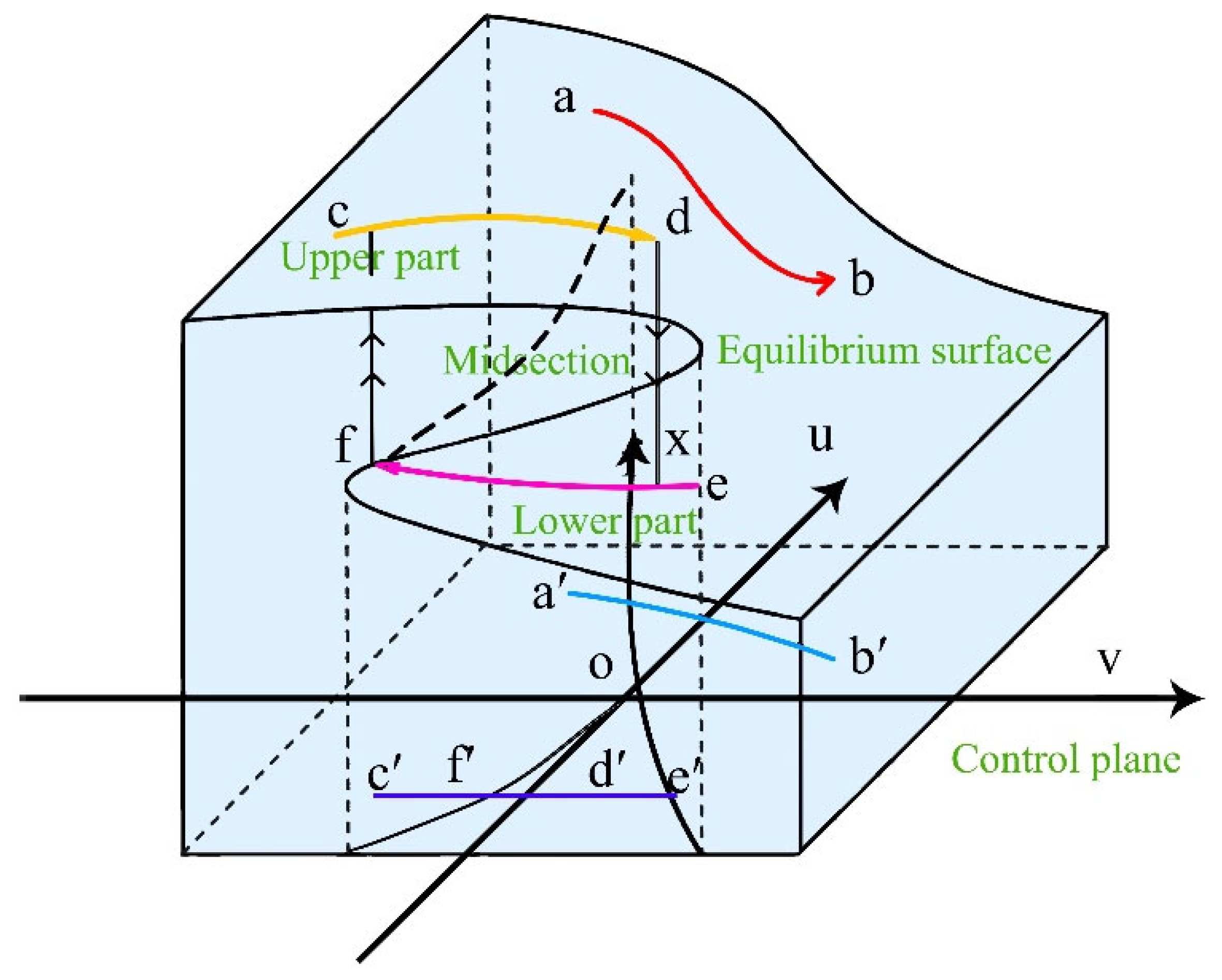
2.2. Singular Point Catastrophe Theory

The singular point catastrophe theory is one of the most widely used theories at present. Its potential function in standard form is [38,39]

$$V_{(x)}=x^4+u{x}^2+vx$$

(9)

In the singular point catastrophe theory, the function V_(x) has u and v as control variables and x as the state variable. Differentiating it yields the equilibrium equation

$${V^{\prime }}_{(x)}=4x^3+2ux+v$$

(10)

According to Figure 1 below, the singular point catastrophe theory model is divided into three parts from bottom to top, forming a curved and folded surface. The curved and folded section can be divided into the lower leaf, middle leaf, and upper leaf. It is evident that the conditions vary in different regions: the upper and lower leaves are equilibrium stable points, while the middle leaf is in an unstable state. Differentiating V_(x) gives us that the singular point set satisfies

$$V_{(x)}^{″}=12x^2+2u=0$$

(11)

At this point, when t is considered, singular points are obtained where the vertical tangent in the equilibrium equation intersects with the curve. Depending on the number of equilibrium positions on the curve, multiple singular points may be obtained. By solving the equations simultaneously and eliminating x, we can derive:

$$\Delta =8u^3+27v^2$$

(12)

This formula represents the discriminant used to determine the critical bifurcation value in the singular point catastrophe theory model.

2.3. Establishment of Destabilization Criteria for Slope Excavation

Dissipation theory suggests that rock damage during slope excavation is the result of energy dissipation. Using the FLAC3D (Version 6.0) finite difference software, after excavating the slope, the energy of the slope can be calculated. This can be achieved either by writing a Fish script to convert using extra or by writing a Fish script to monitor the energy of the model elements [40].

To assess the stability discontinuity of the surrounding rock during the slope excavation, the energy after k steps of excavation can be defined as follows:

$$E_{\mathrm{k}}({\mathrm{a}}^{\mathrm{s}})={\displaystyle \sum _{\mathrm{i}=1}^{\mathrm{n}}{E}_{\mathrm{k}}^{\mathrm{i}}\left({\mathrm{a}}^{\mathrm{s}}\right)}$$

(13)

In the formula, $E_{\mathrm{k}}^{\mathrm{i}}\left({\mathrm{a}}^{\mathrm{s}}\right)$ is the change in energy dissipation density of the unit body after the a^s excavation.

$$V_{(\mathrm{t})}=a_0+a_{1}t+a_2{t}^2+a_3{t}^3+a_4{t}^4$$

(14)

To simplify calculations, real variable functions and complex variable functions are established, and the Laplace transform is used. Let $t=x-A$, $A={\displaystyle \raisebox{1ex}{$a_3$}\!\left/ \!\raisebox{-1ex}{$4a_4$}\right.}$; the resulting relationship is

$$V_{\left(\mathrm{x}\right)}{=\mathrm{b}}_0+b_1\mathrm{x}+b_2{\mathrm{x}}^2+b_4{\mathrm{x}}^4$$

(15)

The relationship between a_i and b_i is given by

$$\begin{array}{l}{\mathrm{b}}_0=A^4{\mathrm{a}}_4-A^3{a}_3+A^2{a}_2-A{a}_1+a_0\\ b_1=-4A^3{a}_4+3A^2{a}_3-2A{a}_2+a_1\\ b_2=6A^2{a}_4-3A{a}_3+a_2\\ b_4=a_4\end{array}$$

(16)

By dividing both sides by b₄, the standard function form of the discontinuity model can be obtained:

$$V_{(x)}=x^4{+\mathrm{ux}}^2+vx+c$$

(17)

In the equation, c is a constant, so it can be simplified to

$$V_{(x)}=x^4{+\mathrm{ux}}^2+vx$$

(18)

where u and v are defined as

$$\mathrm{u}={\displaystyle \frac{a_2}{a_4}}-{\displaystyle \frac{3a_3^2}{8a_4^2}}\mathrm{v}={\displaystyle \frac{a_1}{a_4}}-{\displaystyle \frac{a_2{a}_3}{2a_4^2}}+{\displaystyle \frac{a_3^3}{8a_4^3}}$$

(19)

According to the critical instability judgment criterion of the discontinuity theory, by differentiating $V_{(\mathrm{x})}$ with respect to the relevant variable, and setting $V_{(x)}^{\prime }=0$, $V_{(x)}^{″}=0$, the following can be obtained:

$$8{\mathrm{u}}^3+27{\mathrm{v}}^2=0$$

(20)

At this point, using the aforementioned discontinuity theory for instability judgment, the dissipative energy discontinuity in the slope excavation process can be assessed through $\Delta =8u^3+27v^2$. When Δ > 0, the system is in a stable state; when Δ < 0, the system is in an unstable state; and when Δ = 0, the system is in a critical state. The slope will become unstable when the dissipative energy reaches the discontinuity condition.

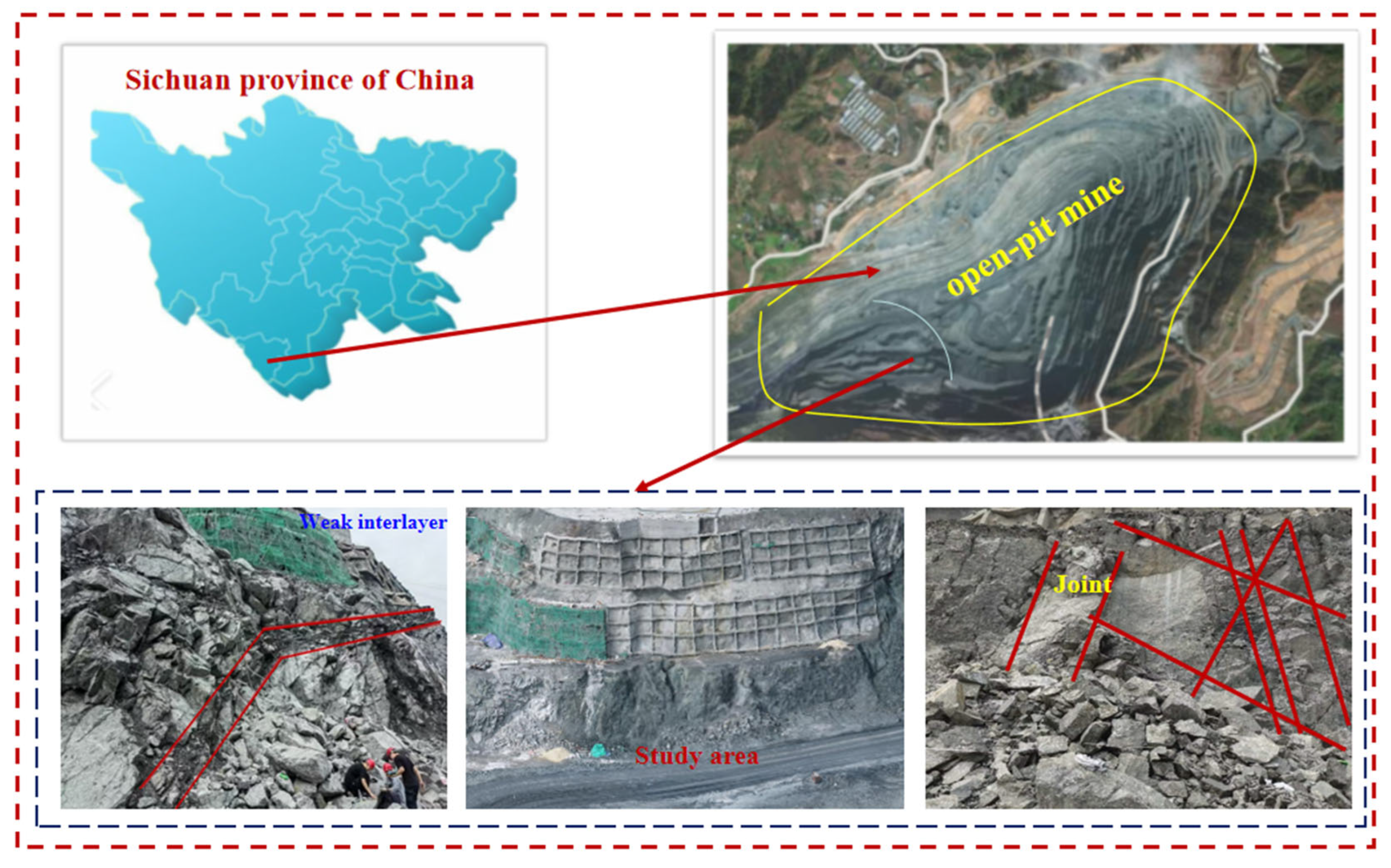
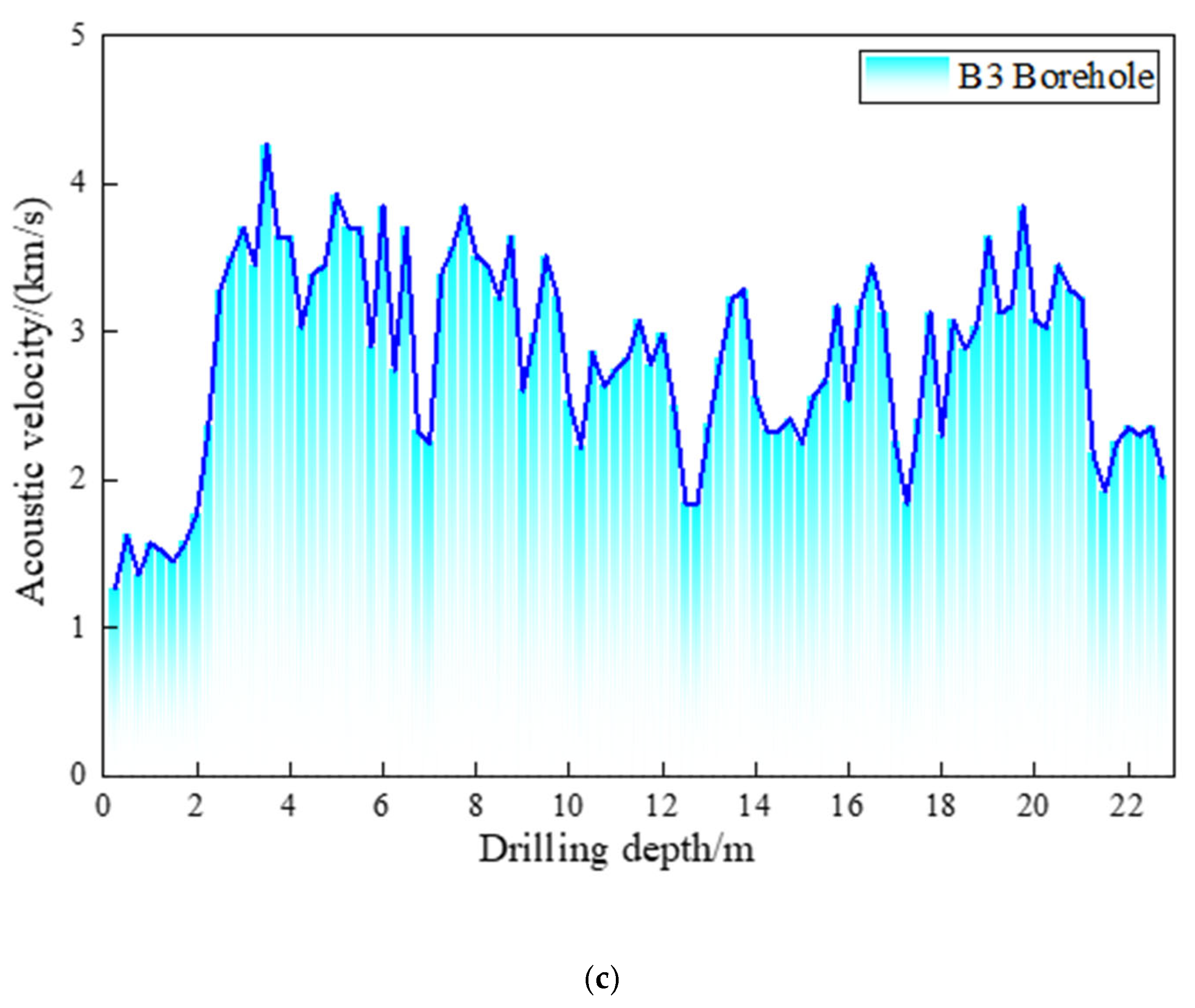
3. Engineering Context and Site Condition

Figure 2 illustrates a schematic representation of the study area. The fault is situated between elevations of 1240 m and 1210 m on the slope, where the 1210 m platform is reinforced with an anchor cable frame beam, forming a two-tier slope protection structure. Anchor cables M1 through M8 have anchorage lengths of 8 m, with free end lengths of 36 m, 32 m, 29 m, 26 m, 25 m, 23 m, 23 m, and 26 m, respectively. The transverse and longitudinal beams of the frame measure 4 m each, and the average prestressing force applied to the anchor cables is approximately 700 kN.

The combined use of a prestressed anchor cable frame beam system as the primary support mechanism forms a three-tier retaining structure. This system is enhanced by anchor cable frame beams arranged in a 4 m × 4 m grid, designed with a prestressing force of 1000 kN and an anchorage angle of 15°. The anchor cables in these reinforced zones have lengths of 58.5 m, 62.5 m, 62.5 m, and 66.5 m, with an anchorage length of 12 m. The frame beams have cross-sectional dimensions of 500 mm × 500 mm, and both transverse and longitudinal beams measure 4 m in length.

Localized slope damage has been observed, primarily attributed to structural surfaces, weak interlayers, and ongoing mining activities.

3.1. Slope Rock Mass Structure Testing Research

The stability of slopes is fundamentally governed by their structural configuration. To enable accurate modeling and effective analysis of slope stability, it is essential to determine the slope’s structure and strength parameters prior to analysis, facilitating predictions of failure patterns and development trends. Geo-radar technology can be utilized for slope monitoring, offering precise detection of weak inclusions and cracks while providing foundational data for 3D modeling. Rock acoustic testing, particularly ultrasonic testing, is extensively applied to evaluate geotechnical parameters, identify faults, detect weak inclusions, and characterize loose zones. This method assesses rock properties by measuring the propagation velocity and attenuation coefficient of sound waves in the rock mass. The principle underlying this technique is that sound waves traversing cracks or interlayers experience an extended propagation path, resulting in reduced wave velocity compared to intact rock, thereby revealing structural changes within the rock mass caused by fracturing. Combined, these techniques serve as critical tools for comprehensive slope stability assessments.

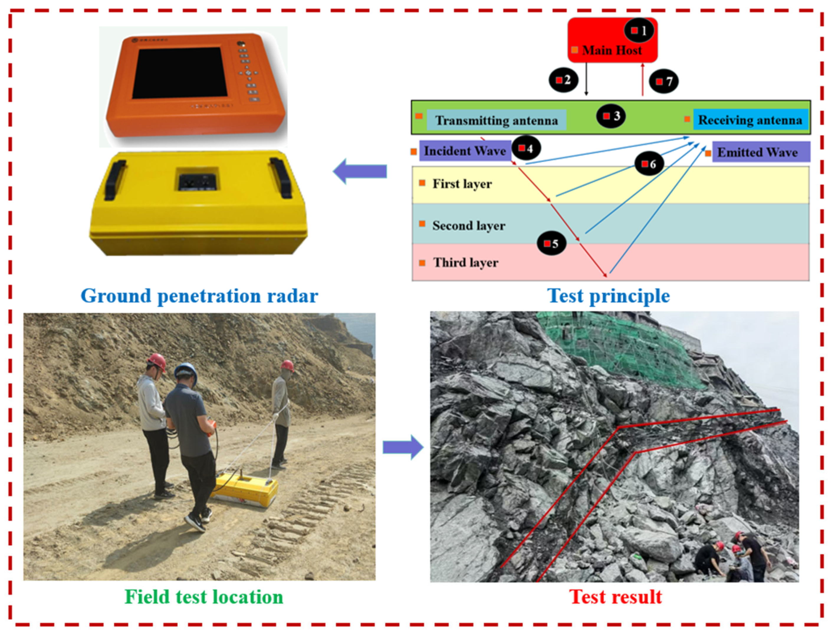
3.1.1. Geological Radar Testing

As depicted in Figure 3, the process flow diagram of the geological radar testing is presented. Considering the site conditions of the transfer station and the mining field slope, the radar method was employed to survey three measurement lines positioned below the mining field floor and three additional lines arranged around the mining field. These measurement lines were located on the left side, the wedge-shaped body, and the right side, respectively. A 900 MHz antenna was utilized, with the time window set between 600 and 700 ns, enabling detection at a depth of 30–35 m. Continuous data acquisition was conducted throughout the testing process.

The depth z of the reflector is automatically calculated using Equation (21) based on the measured radar wave travel time. The range and characteristics of the reflector are then further analyzed and determined.

$$t={\displaystyle \frac{\sqrt{4z^2+x^2}}{v}}$$

(21)

3.1.2. Geological Radar Test Results

(1)

Internal Rock Mass Integrity Analysis of the Transfer Station Slope

Multiple measurement lines were set up at the P01 transfer station and the 1195 platform of the mining field, and radar wave detection technology was employed for a detailed investigation of the surrounding rock’s geological conditions. As shown in Figure 4a–c, which present schematic diagrams of the geological radar test results, the analysis indicates the presence of a fractured zone approximately 4 m thick, located 13 to 17 m below the P01 transfer station. This zone is characterized by poor rock mass integrity and well-developed joints and fissures. Additionally, within the 0 to 13 m range below the 3# measurement line at the transfer station, frequent operations and vibrations have facilitated the development of rock fissures, resulting in the formation of a fractured zone. On the 1195 platform of the mining field, from 0 to 17 m, the rock mass integrity is poor, with well-developed joint fissures and a small amount of bedrock fissure water. In contrast, from 17 to 35 m, the rock mass exhibits better integrity with more developed joint fissures.

(2)

Geological Radar Detection Results for Weak Interlayers

A weak interlayer refers to a layered structure within the rock mass that has a certain thickness and consists of structural surfaces weaker than those of the surrounding rock mass. These interlayers exhibit lower strength and higher compressibility. Although the number of weak interlayers in the rock mass may be limited, they are often the most vulnerable areas, posing potential risks in engineering and significantly impacting the stability of open-pit mine slopes. The main types of interlayers that affect the stability of open-pit mine slopes include sedimentary, metamorphic, weathered, clayey, and secondary clay interlayers, AS shown in

Table 1. Statistics of each weak interlayer.

Weak Structural Surface	Occurrence	Thickness (cm)	Opening Width	Filling Material
L1	160 ∠ 24	35	Large	Chlorite
L2	282 ∠ 46	11~20	Large	Chlorite

is the Statistics of each weak interlayer.

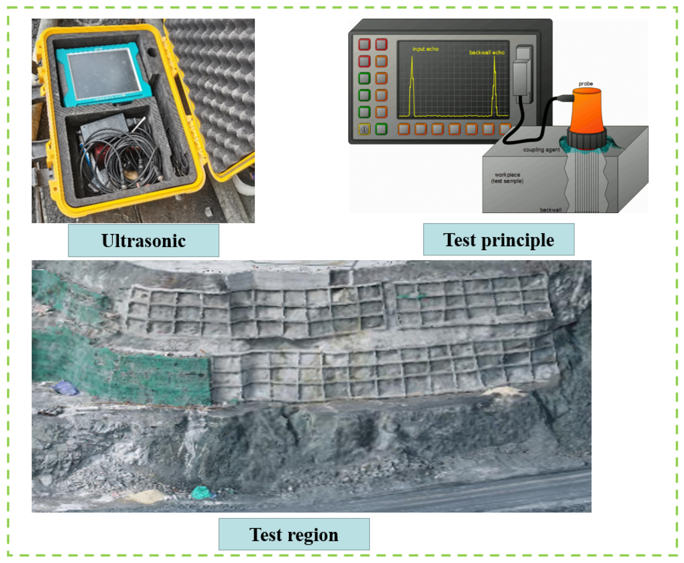
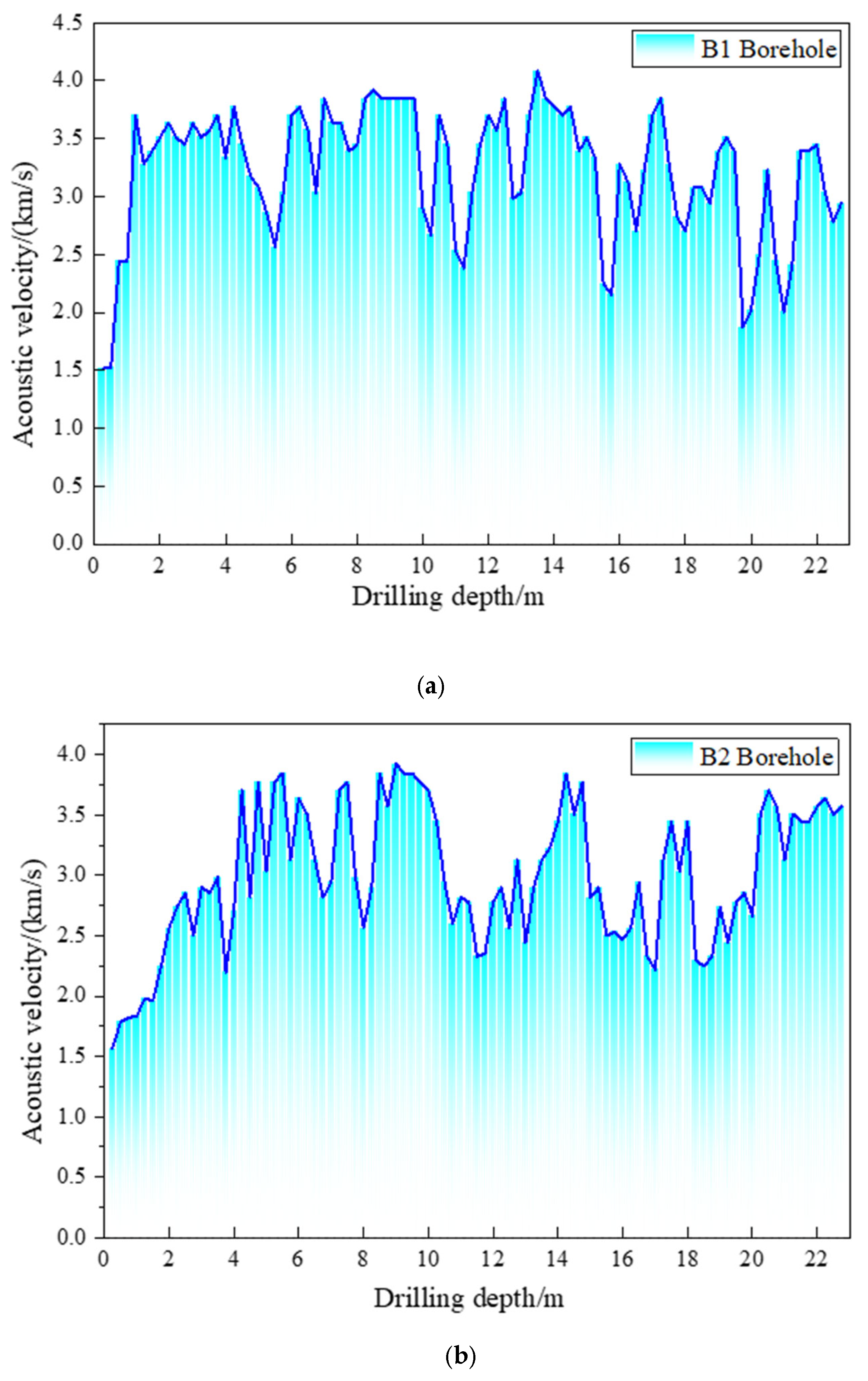
3.2. Acoustic Testing

The acoustic testing of rock masses is widely employed to detect geotechnical parameters, faults, weak interlayers, and loose zones. The principle behind this method is based on the propagation speed and attenuation coefficient of sound waves within the rock mass. By measuring these parameters, the properties of the rock mass can be inferred. In the mining field slope, ultrasonic testing using borehole techniques was utilized. Ultrasonic equipment was used to measure sound wave parameters along the vertical axis, allowing for the analysis of the engineering characteristics of the surrounding rock at various depths. As shown in Figure 5, this is a schematic diagram of the ultrasonic testing process. The RSM-SY7 non-metallic ultrasonic system from Zhongyan Technology was employed, along with its principle diagram, where transmitters and receivers are placed within the rock mass. By transmitting and receiving acoustic pulse signals, characteristics such as changes in acoustic impedance, wave velocity, energy attenuation, frequency variations, and waveform distortions are analyzed to identify the type, size, and location of defects in the rock mass. An acoustic velocity–depth curve is constructed to assess the nature and extent of these defects.

Acoustic Testing Results

The ultrasonic testing results from the field are presented in Figure 6 for the three selected boreholes, as follows:

Figure 6a—B1 Borehole: The measured wave speeds ranged primarily from 2247 m/s to 3846 m/s, with a minimum value of 1566 m/s and a maximum value of 3846 m/s.

Figure 6b—B2 Borehole: The measured wave speeds ranged primarily from 2353 m/s to 3922 m/s, with a minimum value of 1266 m/s and a maximum value of 3922 m/s.

Figure 6c—B3 Borehole: The measured wave speeds ranged primarily from 2439 m/s to 3774 m/s, with a minimum value of 1515 m/s and a maximum value of 4082 m/s.

Based on these test results, it can be inferred that the loose zone in the surrounding rock of Borehole B1 is located approximately between 3.25 and 3.75 m, while the loose zone in Borehole B2 is found between 2.50 and 2.75 m. Additionally, the acoustic velocity data from the surrounding rock predominantly falls within the range of 2500 to 4000 m/s, indicating that the surrounding rock is affected by joint fissures. This results in a blocky and fractured structural characteristic of the rock mass.

4. Numerical Calculation of Slopes Based on Weibull Parameter Random Distribution Model

4.1. Random Distribution Model of Rock Mass Parameters

Based on the results from the geodetic radar and ultrasonic tests, the platform between elevations of 1195 m and 1240 m was divided into three zones: left, center, and right, for modeling calculations. As shown in Figure 7, the calculation model was further subdivided into three sub-zones: Zone I, Zone II, and Zone III for zonal modeling. The model dimensions are 492 m in the X-direction, 80 m in the Y-direction, and 349 m in the Z-direction, with a slope height of 148 m. The simulation follows the Mohr–Coulomb failure criterion, with the building acting as a stress load applied to the top of the slope. The physical and mechanical parameters of the rock mass are provided in

Table 2. Physical and mechanical parameters of the rock mass.

Rock Layer	Young/kPa	Poisson	Cohesion/kPa	Friction Angle/°	Tension/kPa	Density/(KN/m3)
Coarse-Grained Diorite	6.9 × 106	0.26	0.88 × 103	37	0.96 × 103	3.1
Fine-Grained Diorite	6.5 × 106	0.28	0.65 × 103	36	0.87 × 103	3.1
Ore	7.5 × 106	0.26	0.704 × 103	37	0.95 × 103	3.4
Weak Layers	0.8 × 106	0.33	0.02 × 103	24	0.032 × 103	2.5
Zone I	7.01 × 106	0.26	0.72 × 103	36.12	0.26 × 103	3.6
Zone II	2.81 × 106	0.33	0.56 × 103	32.92	0.04 × 103	3.2
Zone III	6.17 × 106	0.27	0.64 × 103	34.89	0.15 × 103	3.22

, excluding the experimentally measured parameters for the platforms between 1195 m and 1240 m.

The calculation steps are as follows:

(1)

Establish the slope numerical calculation model.

(2)

Fix the boundaries on the four sides and the bottom of the model.

(3)

Achieve initial geostatic stress equilibrium.

(4)

Use Fish script to write the code for calculating dissipated energy.

(5)

Extend downward by one step and record the results.

(6)

Repeat the previous step until the excavation reaches the 13th step.

Due to the presence of numerous joints, fractures, and other defects in the rock mass, which belong to nonlinear units, it is difficult to define the initial condition of the units. Therefore, the Weibull distribution is used for definition. The Weibull probability density function [41,42,43,44,45] is given by

$$\mathrm{f}\left(\mathrm{u}\right)=\left\{\begin{array}{ll}{\displaystyle \frac{\mathrm{m}}{{\mathrm{u}}_0}}{({\displaystyle \frac{u}{u_0}})}^{m-1}\exp (-{({\displaystyle \frac{u}{u_0}})}^m& u\ge 0\\ 0& u<0\end{array}\right.$$

(22)

In the equation, u represents the value of the random variable. u₀ is a scale parameter related to the average value of all unit parameters. m is the shape parameter, which defines the shape of the Weibull probability density function.

4.2. Mining Slope Stability Analysis Lower Extension Mining

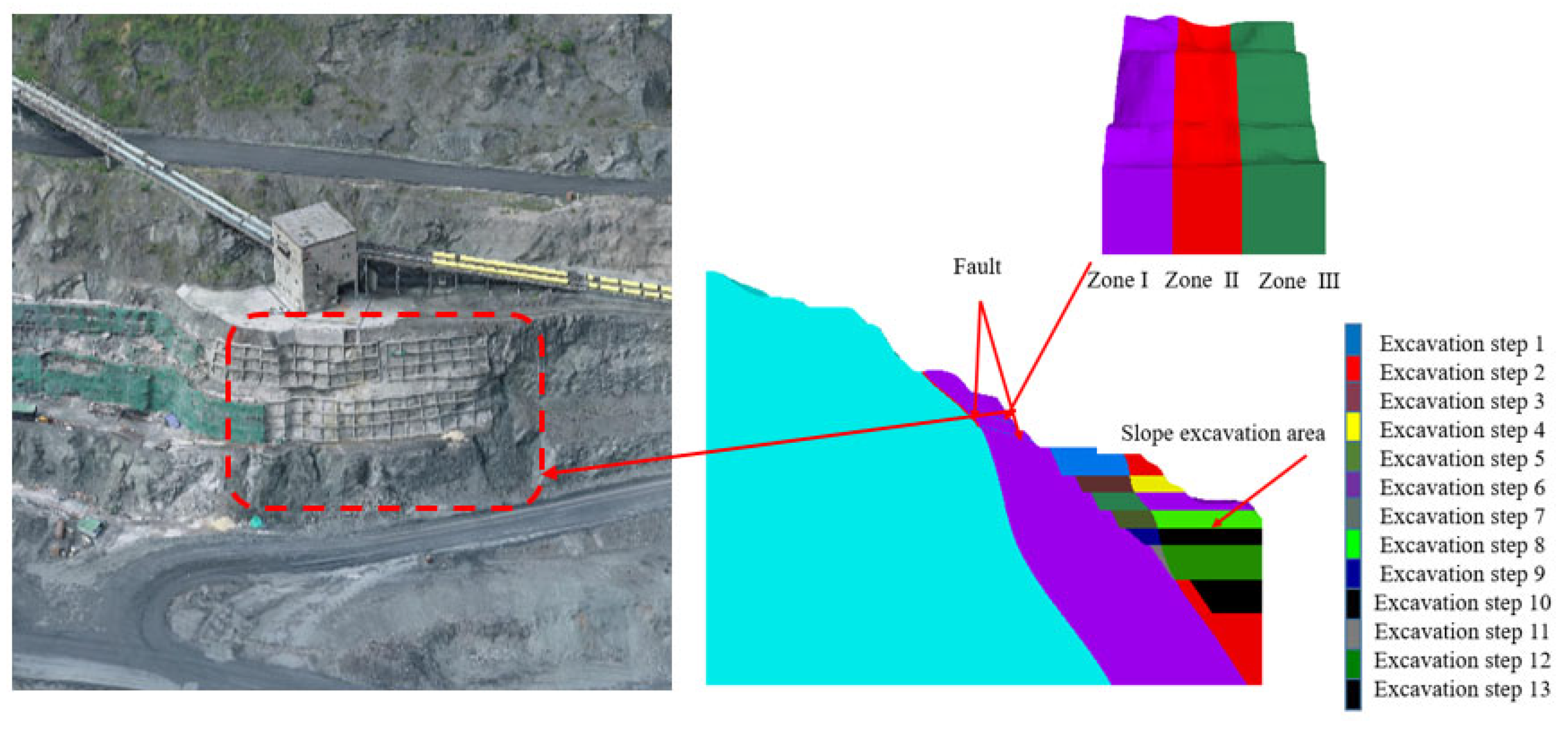
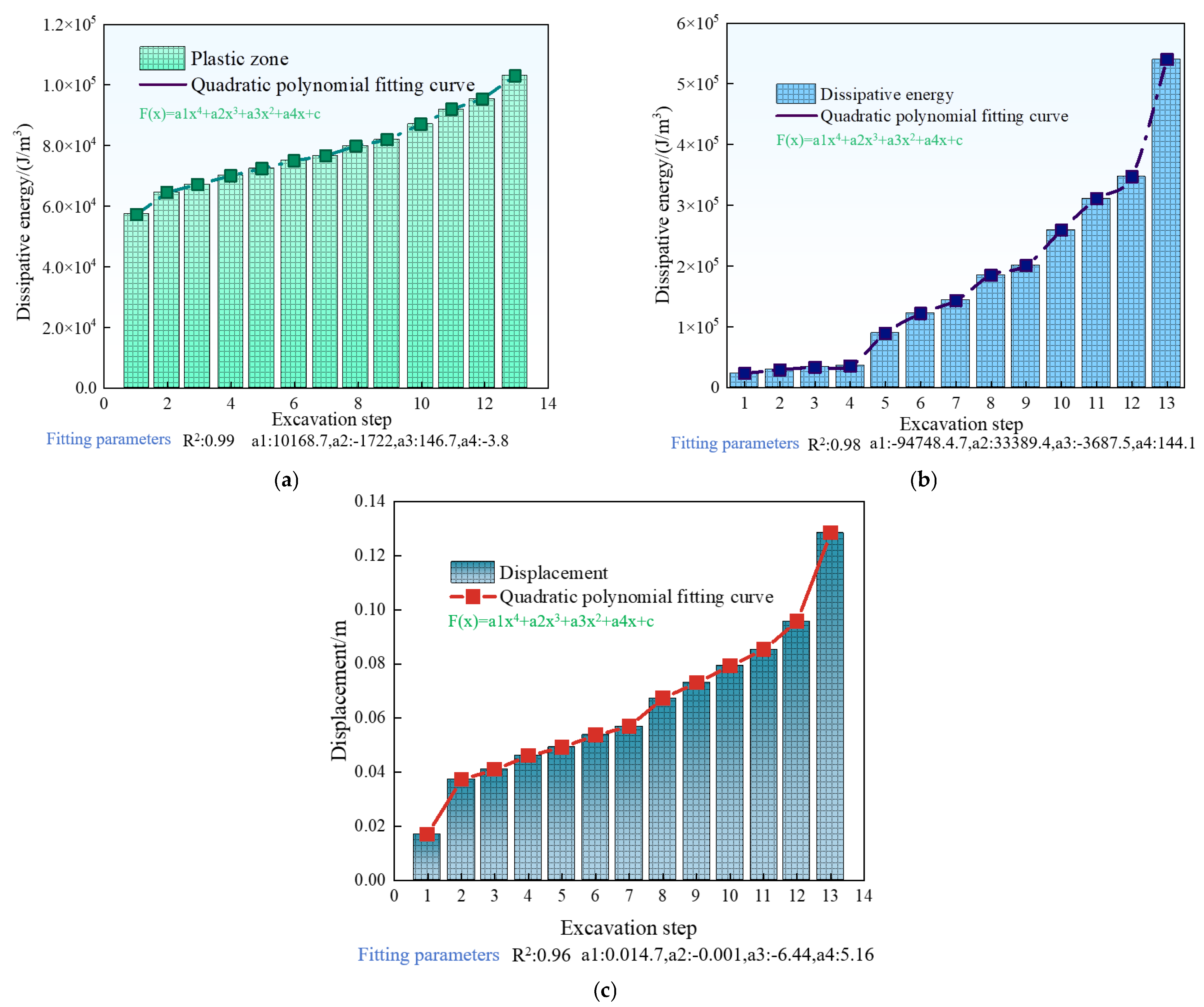
4.2.1. Analysis of Slope Energy Evolution

As shown in Figure 8, during the open-pit mining process, energy dissipation experiences significant changes as excavation progresses downward. Following the initial excavation, the starting energy dissipation value is 0.69 MJ/m³, and it steadily increases with each subsequent excavation stage. By the fourth excavation, the energy dissipation reaches 0.728 MJ/m³, and after the tenth excavation, it further increases to 0.77 MJ/m³, indicating a gradual accumulation of energy dissipation with increasing excavation depth. Notably, when excavation reaches the thirteenth stage, near the pit bottom, energy dissipation sharply spikes to 1.26 MJ/m³. In the slope area between elevations of 1195 m and 1240 m, energy dissipation undergoes a dramatic change. As shown in Figure 8e, the significant increase in energy dissipation after the thirteenth excavation suggests that the energy dissipation zone in the slope rock mass may have fully connected, forming a critical region for energy release and transformation. This pattern of change underscores the profound impact of excavation activities on the geological environment and highlights the potential safety risks associated with such operations.

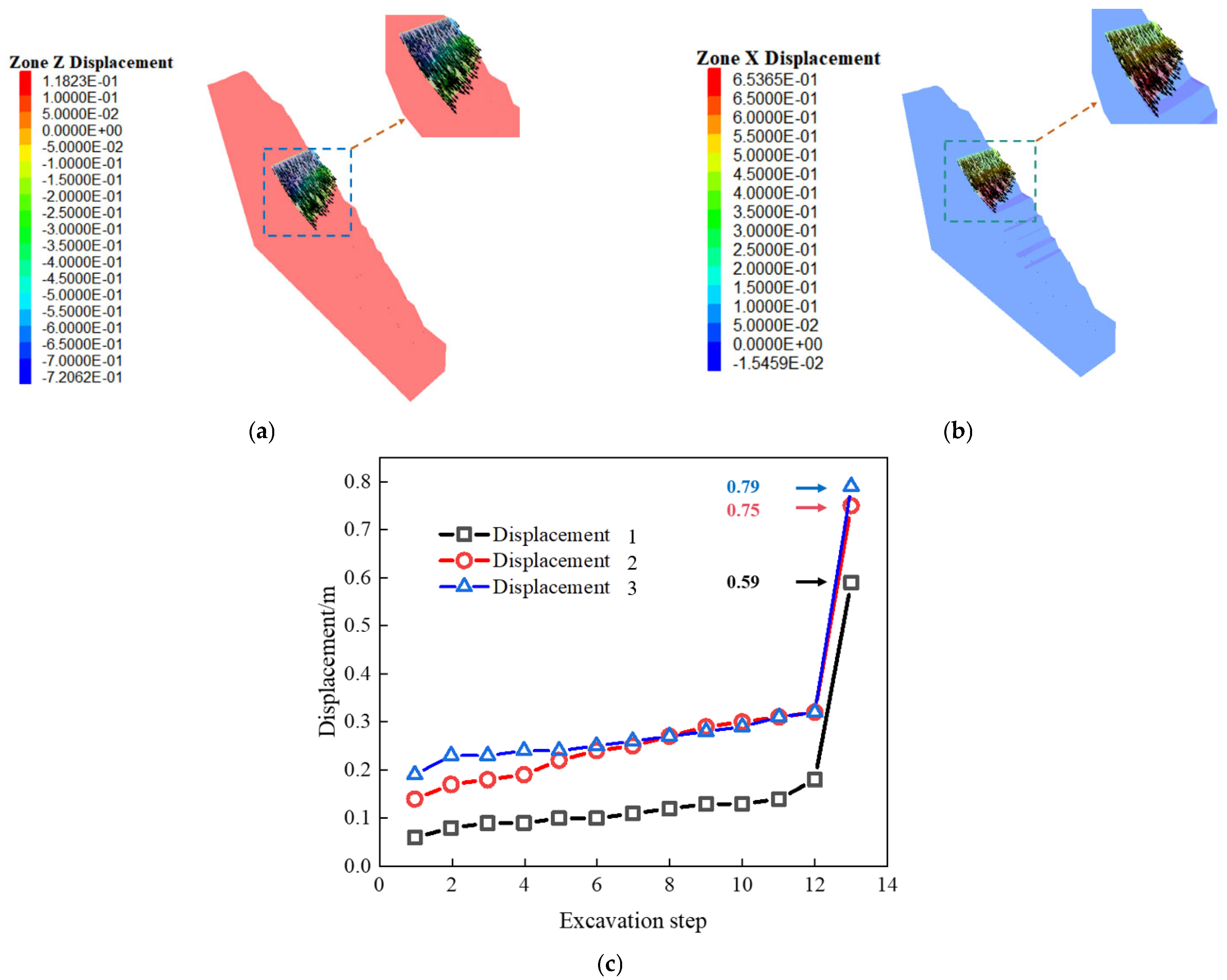
4.2.2. Analysis of Slope Displacement Evolution

As shown in Figure 9a,b, the displacement contour maps in the z-direction and x-direction, respectively, after the completion of slope excavation are presented, while Figure 9c shows the displacement diagrams for each excavation stage. Due to the substantial disturbance caused by excavation activities and the resulting critical surface effects, the slope body inevitably experienced deformation. In the vertical direction, the slope exhibited significant settlement, with a maximum displacement of 72 cm, indicating a clear settlement trend. In the horizontal direction, a displacement of 65 cm was recorded, reflecting considerable deformation. The displacement monitoring curve further reveals a sharp transition during the 13th excavation stage, highlighting a significant shift in the slope structure. This underscores the profound impact of excavation activities on slope stability and the critical transitions that occur during deeper excavation stages.

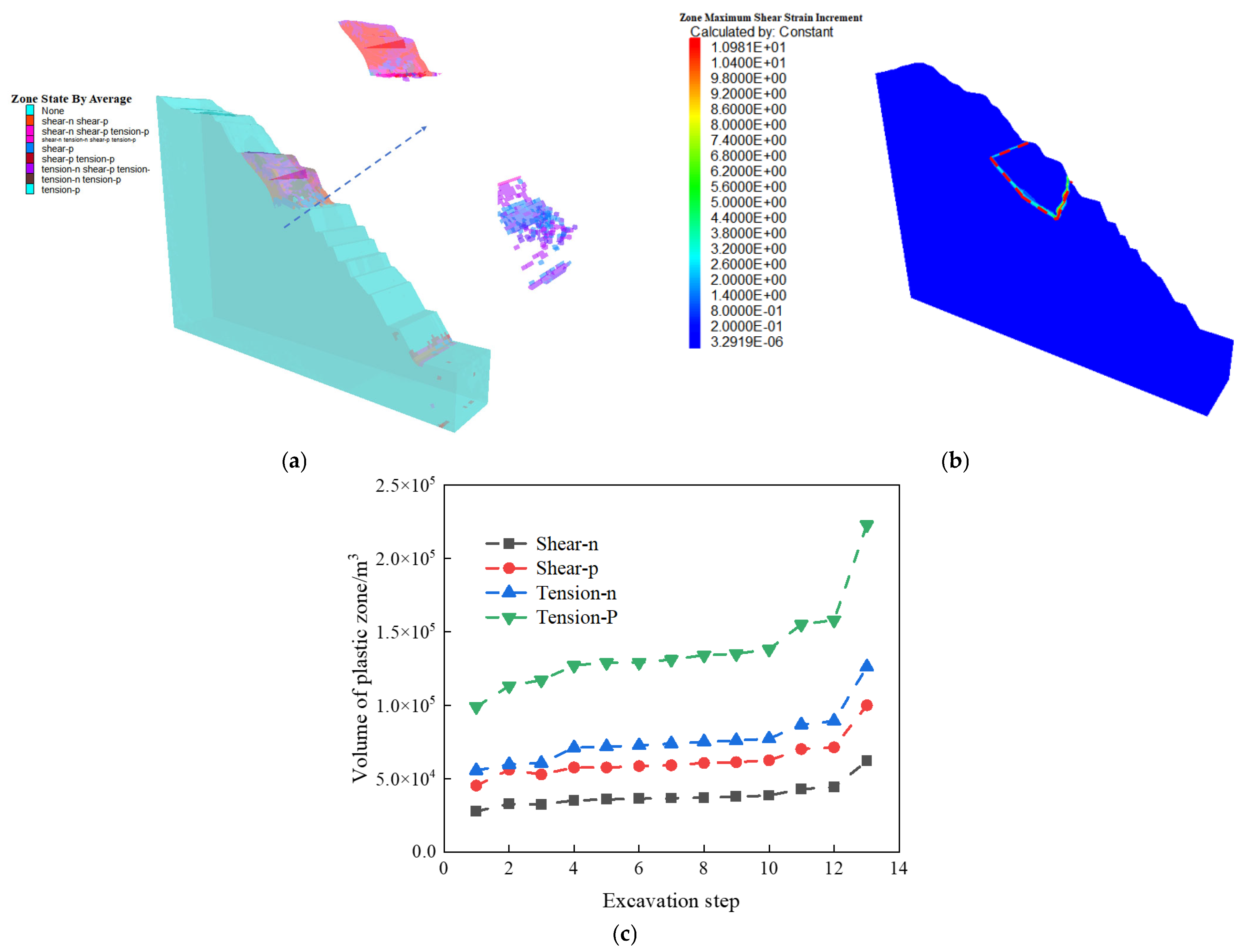
4.2.3. Plastic Zone and Maximum Shear Strain Analysis

As shown in Figure 10a,b, the plastic zone cloud maps and maximum shear strain cloud maps after slope excavation are presented, respectively, while Figure 10c shows the plastic zone volume curve at different excavation stages throughout the excavation process. Analysis reveals that a fully penetrative plastic zone developed in the platform area between elevations 1195 m and 1240 m, indicating severe instability in the soil within this region. The plastic zone volume curve, calculated using Fish scripting, shows a sudden increase in volume. Although a localized plastic zone also formed at the slope toe during mining, it has not yet fully penetrated, displaying localized damage characteristics. The maximum shear strain analysis further supports this finding, as the maximum shear strain in this area also reached a fully penetrative state. These results strongly suggest that excavation activities at the 1195 m to 1240 m platform caused significant disturbance, ultimately leading to the loss of slope stability and subsequent slope failure.

4.3. Slope Stability Analysis Based on Cusp Mutation Theory

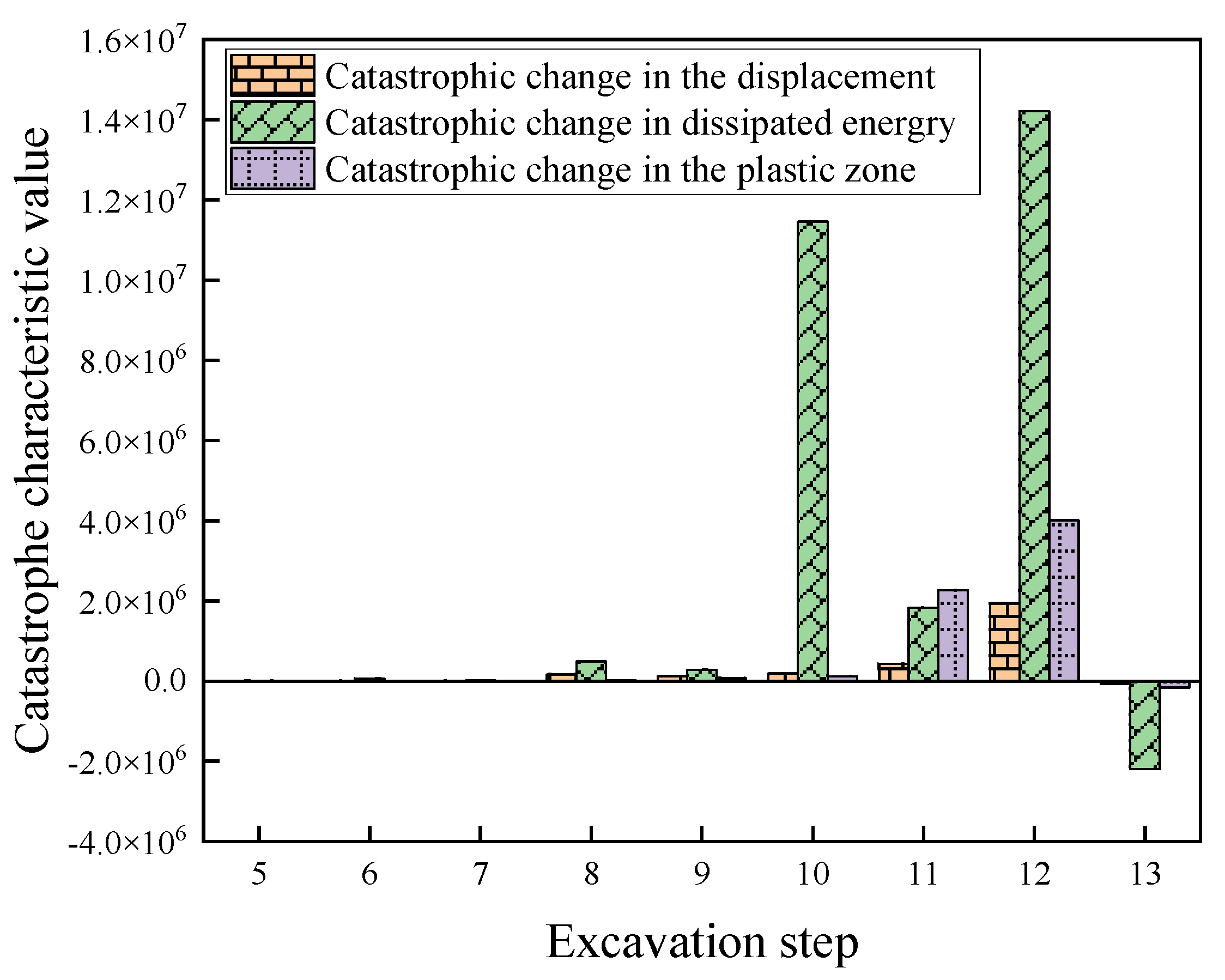
4.3.1. Analysis of Instability and Sudden Change in Slopes with Energy Damage

Due to the inherent characteristics of cusp catastrophe theory, more than four sets of data are required to fit and calculate the eigenvalue Δ using Origin, based on the changes in dissipative energy, displacement, and plastic zone during excavation. From the results of numerical simulations, the variation in dissipated energy of the slope was derived, indicating the energy dissipation at each excavation stage. Using the obtained data, a fourth-degree polynomial fitting was performed to determine the coefficients of each term and calculate the values of u and v. Subsequently, the mutation characteristic values were calculated to assess the slope’s stability.

According to Equation (23),

$$\mathrm{u}={\displaystyle \frac{a_2}{a_4}}-{\displaystyle \frac{3a_3^2}{8a_4^2}}. \mathrm{v}={\displaystyle \frac{a_1}{a_4}}-{\displaystyle \frac{a_2{a}_3}{2a_4^2}}+{\displaystyle \frac{a_3^3}{8a_4^3}}.$$

(23)

4.3.2. Dissipated Energy Mutation Analysis

As shown in Figure 11, the schematic diagram illustrates the variation in the mutation characteristic values of energy dissipation, plastic zone, and displacement. During the slope excavation process, the trends in energy dissipation, plastic zone volume, and displacement collectively reflect the evolution of slope stability. The study indicates that in the early stages of excavation, energy dissipation increases gradually, the growth of the plastic zone volume is limited, and displacement changes are minimal, suggesting that the slope remains in a stable state. However, as excavation progresses, particularly at the 13th excavation stage, energy dissipation experiences a sharp surge, the plastic zone expansion reaches a critical state, and significant displacement occurs. This suggests that the redistribution of internal stress within the slope has triggered nonlinear deformation and stress concentration. According to cusp catastrophe theory, at this stage, the mutation characteristic value Δ shifts from positive to negative, further confirming the transition of the slope from stability to instability. Through a comprehensive analysis of these factors, it can be concluded that the rapid accumulation of energy dissipation serves as a key indicator of energy instability, the expansion of the plastic zone reflects the degradation of the slope’s mechanical properties, and the abrupt increase in displacement directly signals the slope’s transition into an unstable state. Together, these factors elucidate the dynamic mechanism underlying the slope’s shift from stability to instability.

4.3.3. Safety Factor Variation Analysis

A comprehensive analysis of slope stability during the excavation process, using the strength reduction method, is summarized in

Table 3. Corresponding table of mutation eigenvalues and safety coefficients for different excavation steps.

Evaluation Indicators	Excavation Step	u	v	Δ	FOS
Dissipated energy	5	−3	−5	459	1.134
	6	−4	−13	4051	1.121
	7	−6	−21	8835	1.096
	8	−23	−99	167,291	1.075
	9	−19	−81	122,275	1.063
	10	−22	−101	190,243	1.042
	11	−26	−145	427,067	1.034
	12	−43	−309	1,941,931	1.025
	13	−23	−29	−74,629	0.962
Displacement	5	−3	−22	12,852	1.134
	6	−19	−65	59,203	1.121
	7	−6	−24	13,824	1.096
	8	−40	−193	493,723	1.075
	9	−13	−105	280,099	1.063
	10	−19	653	11,458,171	1.042
	11	−60	−363	1,829,763	1.034
	12	−109	−954	14,212,900	1.025
	13	−98.8	−452.3	−2,191,909	0.962
Plastic zone	5	−3	−6	756	1.134
	6	−5	−9	1187	1.121
	7	−8	−24	11,456	1.096
	8	−12	−36	21,168	1.075
	9	−21	−74	73,764	1.063
	10	−22	−87	119,179	1.042
	11	−67	−416	2,266,408	1.034
	12	−69	496	4,014,360	1.025
	13	−28	24	−160,064	0.962

. The results reveal a clear correlation between the factor of safety (FOS), abrupt changes in dissipated energy and displacement, and shifts in the plastic zone distribution. As excavation progresses, the overall stability of the slope significantly declines, as evidenced by a gradual decrease in FOS values. Notably, after the thirteenth excavation stage, the FOS drops to 0.96, indicating a critically stable condition, where the risk of slope failure becomes highly significant.

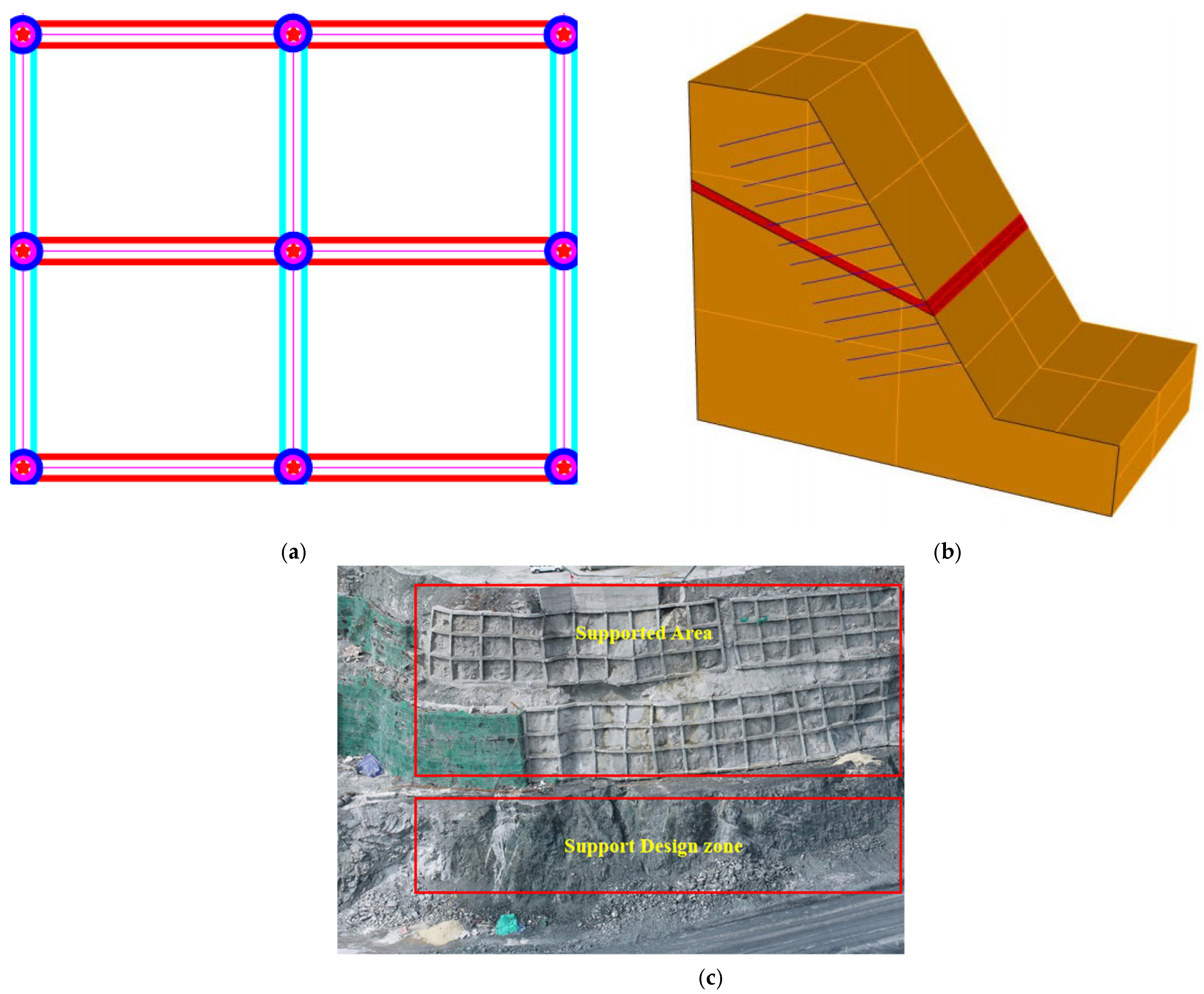
4.4. Slope Stabilization Measures

Due to mining activities, a man-made slope with significant height variations has formed on-site. Some sections of the slope have already been reinforced, but localized damage has occurred in certain areas as mining continues. The transfer station slope system is a crucial transportation route within the mining area, and the P01 transfer station is a key facility in this system, which must remain operational until the completion of open-pit mining. Any damage to the slope could severely compromise the safety of the mining operations. Therefore, to ensure the safe operation of the transfer station, permanent slope support measures are necessary. A schematic diagram of the anchor framework beam is shown in Figure 12.

Anchors are the most commonly used support method for open-pit mining slopes, and they directly affect slope safety and support costs. Therefore, the choice of anchor parameters is crucial. The length of the anchors is key to achieving effective support 38–39. In the slope anchor support design, if the length of the anchor does not penetrate the fractured zone, the support will be ineffective. The anchor length must exceed the range of the fractured zone to fully achieve the support effect. Similarly, if the anchor length is too long, the support effect will not increase significantly and may result in wasted financial and physical resources. Therefore, an anchor framework beam is chosen to support the 1195–1240 m slope; the support parameters are shown in

Table 4. Physical and mechanical parameters of anchor cable grout.

Zone	Young/Gpa	Poisson	Cross-Sectional Area/m2	Prestress/KN	Anchorage Length/m
Supported Area	200	0.2	2.39 × 10−3	1000 KN	44
Support Design zone	200	0.2	2.39 × 10−3	1000 KN	50

and

Table 5. Calculation parameters for frame beam elements.

Young/Gpa	Poisson	Cross-Sectional Area/m2
24	0.2	0.2025

.

4.4.1. Research on Slope Stability Based on the Theory of Singular Point Mutation

As shown in Figure 13a–c, the fourth-order polynomial fitting results for the dissipated energy, plastic zone, and displacement variation curves under the support effect are presented. These figures illustrate the changes in dissipated energy during the excavation of the slope. As excavation progresses, the dissipated energy between 1195 m and 1240 m gradually increases. When excavation reaches the pit bottom, the maximum dissipated energy value reaches 540,650 MJ/m³. The plastic zone volume at this stage is 103,022 m³, and the displacement is 12 cm. As shown in

Table 6. Correspondence table of safety factor and cusp catastrophe theory eigenvalues.

Evaluation Indicators	u	v	Δ	Fos
Dissipative energy	−105.7	−1116.7	777,566,612.7	1.31
Displacement	−0.5798	0.2726	0.447	1.31
Plastic zone	−14.5	215.7	1,231,826.23	1.31

, the analysis indicates that due to the support effect, dissipated energy in the lower part of the excavation significantly decreases. The results in Table 6 show that the bifurcation eigenvalues for dissipated energy, displacement, and plastic zone volume are all Δ > 0. Based on the strength reduction method, the safety factor of the slope is calculated to be 1.31, indicating that under supported conditions, the safety factor of the slope is significantly improved, and the slope remains stable.

4.4.2. Rock Energy Damage Analysis

As shown in Figure 14a,b, the system energy loss variable cloud maps at excavation steps 4 and 13 under unsupported conditions are presented, while Figure 14c,d show the system energy loss variable cloud maps at the same excavation steps under supported conditions. In the unsupported slope, as excavation progresses, the maximum damage variable (ds) of 0.82 is observed in the 1195–1240 m platform area, specifically at the weak interlayer chlorite position, where the unit body’s damage variable is larger. After support is applied, with continued excavation, the damage volume significantly decreases, and ds reduces to 0.48. This suggests that under supported conditions, the slope remains in a stable state. From the perspective of energy damage evolution, the support system effectively meets the actual engineering requirements.

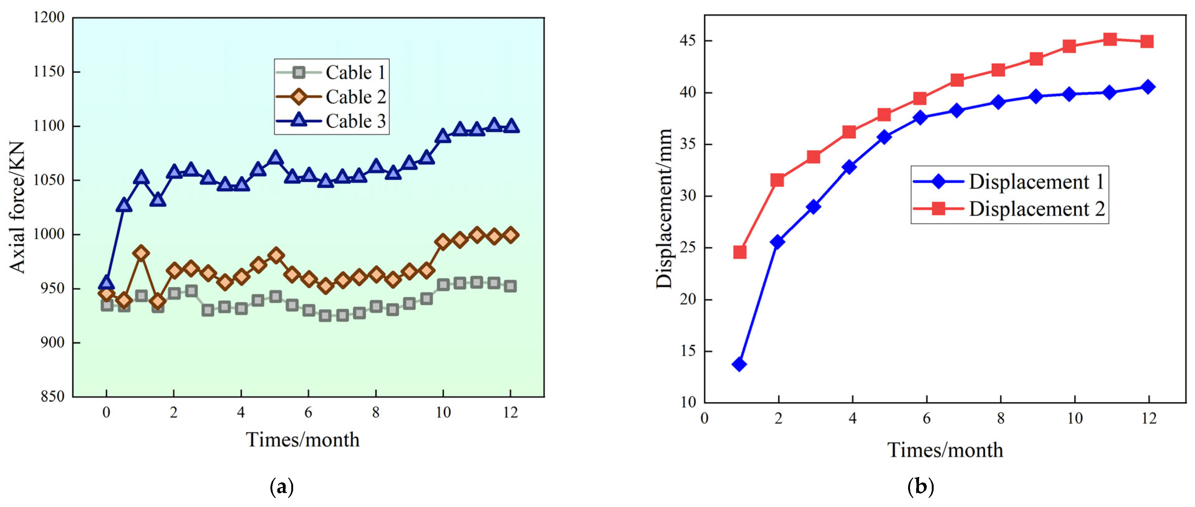
4.5. Field Verification of Anchor Cable Axial Force and Slope Displacement Monitoring

After reinforcement, the stress concentration in localized areas of the slope was effectively alleviated. The anchor framework beam integrated various sections of the slope into a cohesive structural system, significantly enhancing the overall stability of the slope and ensuring its stability under supported conditions.

Slope displacement monitoring provides critical data on slope movement and deformation, which is essential for predicting and preventing potential landslides and collapses [46]. Simultaneously, monitoring the axial force of anchor bolts reflects their stress state and anchoring effectiveness, which is equally vital for ensuring slope stability and preventing anchor bolt failure.

As shown in Figure 15a, the axial force changes in Cable 1 and Cable 2 are relatively small due to their location in the break angle area, while Cable 3, located on the 1240 m platform, exhibits significant axial force changes during production. According to Figure 15b, the blasting dynamic load during production causes some deformation. A comprehensive analysis of the displacement monitoring data reveals that although slope displacement increased during production, the overall magnitude of change was relatively small, indicating that the slope structure remained stable under the implemented support measures.

5. Conclusions

This study investigates the rock mass structure and geological characteristics of a slope in an open-pit mine using acoustic testing, ground-penetrating radar, mutation theory, and energy conservation principles. The Weibull distribution was employed to simulate parameter uncertainty, and a dissipative energy mutation model based on cusp catastrophe theory was utilized to assess the slope stability at the 1195–1240 m platform during excavation. The key findings are as follows:

Acoustic Testing: Loose rock zones range from 2.50 to 3.75 m, with acoustic velocities between 2500 and 4000 m/s, indicating widespread jointing and a fragmented structure.

Numerical Calculation: Dissipated energy and displacement increase during excavation, with a factor of safety (FOS) of 0.962 indicating instability before support, and 1.31 after the installation of the anchor frame beam, confirming stability.

Energy Damage: Maximum damage (ds = 0.82) occurs in the weak chlorite interlayer before excavation, decreasing to ds = 0.48 after support.

Field Monitoring: Displacement and anchor rod axial force data show stability improvements post-support.

These findings demonstrate the effectiveness of support measures in enhancing slope stability.

Furthermore, considering the complexity of engineering practice, future research should explore the environmental sustainability and economic feasibility of the support system, assessing material efficiency and ecological benefits. In addition, practical challenges in applying mutation theory during field monitoring warrant further case studies and technical optimization to improve monitoring accuracy and early warning capability. Lastly, the long-term durability of support measures and their ability to ensure slope stability under evolving climatic and geological conditions should be systematically evaluated to provide comprehensive theoretical support and technical guidance for slope engineering under complex conditions.

References

1. Chen, J.; Li, K.; Chang, K.-J.; Sofia, G.; Tarolli, P. Open-pit mining geomorphic feature characterisation. Int. J. Appl. Earth Obs. Geo Inf. 2015, 42, 76–86. [Google Scholar] [CrossRef]
2. Wang, S.; Cao, B.; Bai, R.; Liu, G. Dynamic optimization design of open-pit mine full-boundary slope considering uncertainty of rock mass strength. Sci. Rep. 2024, 14, 19710. [Google Scholar] [CrossRef] [PubMed]
3. Lin, Y.; Zhou, K.; Li, J. Prediction of slope stability using four supervised learning methods. IEEE Access 2018, 6, 31169–31179. [Google Scholar] [CrossRef]
4. Löbmann, M.T.; Geitner, C.; Wellstein, C.; Zerbe, S. The influence of herbaceous vegetation on slope stability—A review. Earth-Sci. Rev. 2020, 209, 103328. [Google Scholar] [CrossRef]
5. Cao, Y.; Yu, Q.; Yang, T.; Zhu, W.; Le, Z. Numerical study on the fracturing mechanism of the belt conveyor roadway in dagushan Open-Pit mine and control measures evaluation. Rock Mech. Rock Eng. 2022, 55, 6663–6682. [Google Scholar] [CrossRef]
6. Huang, A.; Zhu, Y.P.; Ye, S.H.; Fang, G.G. Three-dimensional stability of a fill slope reinforced by a frame beam anchor plate. Sci. Rep. 2024, 14, 25250. [Google Scholar] [CrossRef]
7. Ohtsuka, S.; Miyata, Y.; Ikemoto, H.; Iwabe, T. Slope Stability Analysis with Rigid-Plastic Finite Element Method. Landslides 2001, 38, 235–243. [Google Scholar] [CrossRef]
8. Bezie, G.; Chala, E.T.; Jilo, N.Z.; Birhanu, S.; Berta, K.K.; Assefa, S.M.; Gissila, B. Rock slope stability analysis of a limestone quarry in a case study of a National Cement Factory in Eastern Ethiopia. Sci. Rep. 2024, 14, 18541. [Google Scholar] [CrossRef]
9. Zhang, Z.; Mei, G.; Xu, N. A geometrically and locally adaptive remeshing method for finite difference modeling of mining-induced surface subsidence. J. Rock Mech. Geotech. Eng. 2022, 14, 219–231. [Google Scholar] [CrossRef]
10. Xu, G.-J.; Zhong, K.-Z.; Fan, J.-W.; Zhu, Y.-J.; Zhang, Y.-Q. Stability analysis of cohesive soil embankment slope based on discrete element method. J. Central South Univ. 2020, 27, 1981–1991. [Google Scholar] [CrossRef]
11. Lianheng, Z.; Dongliang, H.; Shuaihao, Z.; Xiao, C.; Yibo, L.; Min, D. A new method for constructing finite difference model of soil-rock mixture slope and its stability analysis. Int. J. Rock Mech. Min. Sci. Géoméch. Abstr. 2021, 138, 104605. [Google Scholar] [CrossRef]
12. Wang, J.; Li, H.; Jiang, Y.; Tian, P.; Cao, A.; Long, Y.; Liu, X.; Si, P. Slope monitoring optimization considering three-dimensional deformation and failure characteristics using the strength reduction method: A case study. Sci. Rep. 2023, 13, 4049. [Google Scholar] [CrossRef] [PubMed]
13. I Urbancic, T.; Trifu, C.-I. Recent advances in seismic monitoring technology at Canadian mines. J. Appl. Geophys. 2000, 45, 225–237. [Google Scholar] [CrossRef]
14. Li, Y.; Zhu, G.; Zhang, Q.; Rodríguez, A.R. An investigation of integrating the finite element method (FEM) with grey system theory for geotechnical problems. PLoS ONE 2022, 17, e0270400. [Google Scholar] [CrossRef]
15. Foong, L.K.; Moayedi, H. Slope stability evaluation using neural network optimized by equilibrium optimization and vortex search algorithm. Eng. Comput. 2022, 38, 1269–1283. [Google Scholar] [CrossRef]
16. Salunkhe, D.P.; Bartakke, R.N.; Chvan, G.; Kothavale, P.R.; Digvijay, P. An overview on methods for slope stability analysis. Int. J. Eng. Res. Technol. (IJERT) 2017, 6, 2278-0181. [Google Scholar]
17. Deng, D.-P.; Zhao, L.-H.; Li, L. Limit equilibrium method for slope stability based on assumed stress on slip surface. J. Central South Univ. 2016, 23, 2972–2983. [Google Scholar] [CrossRef]
18. Li, S.C.; Zhou, Z.Q.; Ye, Z.H.; Li, L.P.; Zhang, Q.Q.; Xu, Z.H. Comprehensive geophysical prediction and treatment measures of karst caves in deep buried tunnel. J. Appl. Geophys. 2015, 116, 247–257. [Google Scholar] [CrossRef]
19. Zhang, W.; Li, H.; Han, L.; Chen, L.; Wang, L. Slope stability prediction using ensemble learning techniques: A case study in Yunyang County, Chongqing, China. J. Rock Mech. Geotech. Eng. 2022, 14, 1089–1099. [Google Scholar] [CrossRef]
20. Guo, Q.F.; Pan, J.L.; Cai, M.F.; Zhang, Y. Analysis of progressive failure mechanism of rock slope with locked section based on energy theory. Energies 2020, 13, 1128. [Google Scholar] [CrossRef]
21. Mo, Z.; Liu, B.; Zhu, J.; Rao, P. Slope Stability Analysis Using Energy Method Combined with Radial Strip Division Method. J. Univ. Shanghai Sci. Technol. 2020, 42, 63–69. [Google Scholar]
22. Liao, Y.; Deng, T.; Zhang, W.; Xu, Z. Research on the stability and support of peripheral rock in roadway excavation based on the theory of cusp mutation. Nonferrous Met. Eng. 2022, 12, 116–123. [Google Scholar]
23. Intrieri, E.; Carlà, T.; Gigli, G. Forecasting the time of failure of landslides at slope-scale: A literature review. Earth-Sci. Rev. 2019, 193, 333–349. [Google Scholar] [CrossRef]
24. Yang, K.; Wang, T.; Ma, Z. Application of cusp catastrophe theory to reliability analysis of slopes in open-pit mines. Min. Sci. Technol. 2010, 20, 71–75. [Google Scholar] [CrossRef]
25. Guo, Y.; Yuan, G.; Che, A.; Wu, Z.; Zhou, H.; Liu, Y. Reconstruction method for a three-demensional discrete element numerical model of landslides using an integrated multi-electrode resistivity tomography method and an unmanned aerial vehicle survey. J. Appl. Geophys. 2024, 228, 105469. [Google Scholar] [CrossRef]
26. Yang, K.; Shi, C.; Wang, J.F. Applying Catastrophe Theory to Slope Reliability Analysis. Boundaries of Rock Mechanics; CRC Press: Boca Raton, FL, USA, 2008; pp. 577–582. [Google Scholar]
27. Mauldon, M.; Arwood, S.; Pionke, C.D. Energy approach to rock slope stability analysis. J. Eng. Mech. 1998, 124, 395–404. [Google Scholar] [CrossRef]
28. Chen, M.-L.; Zhou, J.-W.; Yang, X.-G. A novel approach for slope stability evaluation considering landslide dynamics and its application to reservoir landslide. Nat. Hazards 2024, 120, 3589–3621. [Google Scholar] [CrossRef]
29. Asteris, P.G.; Rizal, F.I.M.; Koopialipoor, M.; Roussis, P.C.; Ferentinou, M.; Armaghani, D.J.; Gordan, B. Slope stability classification under seismic conditions using several tree-based intelligent techniques. Appl. Sci. 2022, 12, 1753. [Google Scholar] [CrossRef]
30. Xu, N.W.; Dai, F.; Liang, Z.Z.; Zhou, Z.; Sha, C.; Tang, C.A. The dynamic evaluation of rock slope stability considering the effects of microseismic damage. Rock Mech. Rock Eng. 2014, 47, 621–642. [Google Scholar] [CrossRef]
31. Cardarelli, E.; Marrone, C.; Orlando, L. Evaluation of tunnel stability using integrated geophysical methods. J. Appl. Geophys. 2003, 52, 93–102. [Google Scholar] [CrossRef]
32. Sainoki, A.; Mitri, H.S. Simulating intense shock pulses due to asperities during fault-slip. J. Appl. Geophys. 2014, 103, 71–81. [Google Scholar] [CrossRef]
33. Qin, S.; Wang, S.; Jiao, J.J. A cusp catastrophe model of instability of slip-buckling slope. Rock Mech. Rock Eng. 2001, 34, 119–134. [Google Scholar] [CrossRef]
34. Thomas, J.; Gupta, M.; Prusty, G. Assessing global parameters of slope stability model using Earth data observations for forecasting rainfall–induced shallow landslides. J. Appl. Geophys. 2023, 212, 104994. [Google Scholar] [CrossRef]
35. Chen, D.-G.; Gao, H.; Ji, C.; Chen, X. Stochastic cusp catastrophe model and its Bayesian computations. J. Appl. Stat. 2021, 48, 2714–2733. [Google Scholar] [CrossRef]
36. Qi, Y.; Tian, G.; Bai, M.; Song, L. Research on construction deformation prediction and disaster warning of karst slope based on mutation theory. Sci. Rep. 2022, 12, 15182. [Google Scholar] [CrossRef]
37. Li, C.C.; Zhao, T.; Zhang, Y.; Wan, W. A study on the energy sources and the role of the surrounding rock mass in strain burst. Int. J. Rock Mech. Min. Sci. Géoméch. Abstr. 2022, 154, 105114. [Google Scholar] [CrossRef]
38. Lann, T.; Bao, H.; Lan, H.; Zheng, H.; Yan, C.; Peng, J. Hydro-mechanical effects of vegetation on slope stability: A review. Sci. Total Environ. 2024, 926, 171691. [Google Scholar] [CrossRef]
39. Zhou, Z.; Zhou, Y.; Chen, Z. New energy criterion for rock slope excavation-induced failure based on catastrophe theory: Methodology and applications. Bull. Eng. Geol. Environ. 2024, 83, 140. [Google Scholar] [CrossRef]
40. Chen, Q.; Xu, R. Slope stability analysis based on finite element strength reduction theory. Adv. Front. Res. Eng. Struct. 2023, 2, 77–83. [Google Scholar]
41. Li, L.; Tang, C.; Zhu, W.; Liang, Z. Numerical analysis of slope stability based on the gravity increase method. Comput. Geotech. 2009, 36, 1246–1258. [Google Scholar] [CrossRef]
42. Deng, D.-P.; Li, L.; Zhao, L.-H. Stability analysis of slopes reinforced with anchor cables and optimal design of anchor cable parameters. Eur. J. Environ. Civ. Eng. 2021, 25, 2425–2440. [Google Scholar] [CrossRef]
43. Jia, Z.; Tao, L.; Bian, J.; Wen, H.; Wang, Z.; Shi, C.; Zhang, H. Research on influence of anchor cable failure on slope dynamic response. Soil Dyn. Earthq. Eng. 2022, 161, 107435. [Google Scholar] [CrossRef]
44. Pei, H.; Zhang, S.; Borana, L.; Zhao, Y.; Yin, J. Slope stability analysis based on real-time displacement measurements. Measurement 2019, 131, 686–693. [Google Scholar] [CrossRef]
45. Li, G.; Li, N.; Yu, C.; He, M. Bearing capacity behaviour of prestressed anchor cable under slope blasting excavation. Arab. J. Geosci. 2021, 14, 1–16. [Google Scholar] [CrossRef]
46. Osasan, K.S.; Afeni, T.B. Review of surface mine slope monitoring techniques. J. Min. Sci. 2010, 46, 177–186. [Google Scholar] [CrossRef]
Figure 1. Equilibrium surfaces and control planes.
Applsci 15 07304 g001
Figure 2. Diagram of the study area and hazard sources.
Applsci 15 07304 g002
Figure 3. Principle diagram of geological radar detection.
Applsci 15 07304 g003
Figure 4. Radar detection results at the transfer station. (a) Line 1 schematic diagram of geological radar test results; (b) Line 2 schematic diagram of geological radar test results; (c) Line 3 schematic diagram of geological radar test results.
Applsci 15 07304 g004
Figure 5. Schematic diagram of the single transmitter and dual receiver ultrasonic testing.
Applsci 15 07304 g005
Figure 6. Schematic diagram of ultrasonic testing. (a) B1 Borehole ultrasonic testing results; (b) B2 Borehole ultrasonic testing results; (c) B3 Borehole ultrasonic testing results.
Applsci 15 07304 g006aApplsci 15 07304 g006b
Figure 7. Numerically calculated 3D model and distribution of stochastic parameters.
Applsci 15 07304 g007
Figure 8. Dissipated energy cloud during slope excavation: Step 2, Step 4, Step 10, Step 13, and dissipated energy monitoring histogram. (a) Dissipated energy cloud in Step 2 of excavation; (b) dissipated energy cloud in Step 4 of excavation; (c) dissipated energy cloud in Step 10 of excavation; (d) dissipated energy cloud in Step 13 of excavation; (e) bar chart of dissipated energy for different excavation steps.
Applsci 15 07304 g008
Figure 9. Displacement contour map after slope excavation and displacement curve during excavation. (a) Displacement contour map in the z-direction of the slope excavation to the bottom of the pit; (b) displacement contour map in the x-direction of the slope excavation to the bottom of the pit; (c) displacement monitoring curve of the slope excavation to the bottom of the pit.
Applsci 15 07304 g009
Figure 10. The plastic zone, maximum shear strain contour map, and statistical curve of the plastic zone after slope excavation completion. (a) Plastic zone contour map of the slope excavation to the bottom of the pit; (b) maximum shear strain contour map of the slope excavation to the bottom of the pit; (c) volume monitoring curve of the plastic zone from the slope excavation to the bottom of the pit.
Applsci 15 07304 g010
Figure 11. Trend of changes in dissipated energy, displacement, and plastic zone mutation characteristic values.
Applsci 15 07304 g011
Figure 12. Slope support model diagram. (a) Anchor cable frame beam plane schematic diagram; (b) anchor cable frame beam cross-sectional schematic diagram; (c) support schematic diagram.
Applsci 15 07304 g012
Figure 13. Fitted curves of plastic zone, displacement, and energy dissipation under support. (a) Plastic zone fitting curve schematic diagram; (b) dissipated energy fitting curve schematic diagram; (c) displacement fitting curve schematic diagram.
Applsci 15 07304 g013
Figure 14. Energy damage variable contour map of slope elements before support. (a) Energy consumption and damage variable contour map of the slope excavation at the 4th step under unsupported condition; (b) energy consumption and damage variable contour map of the slope excavation at the 13th step under unsupported condition; (c) energy consumption and damage variable contour map of the slope excavation at the 4th step under supported condition; (d) energy consumption and damage variable contour map of the slope excavation at the 13th step under supported condition.
Applsci 15 07304 g014
Figure 15. Displacement monitoring curve. (a) Slope anchor cable axial force monitoring schematic diagram; (b) slope displacement monitoring schematic diagram.
Applsci 15 07304 g015