XSQ-Learning: Adaptive Similarity Thresholds for Accelerated and Stable Q-Learning

Abstract

Reinforcement Learning (RL) enables agents to learn optimal policies through environment interaction, with Q-learning being a fundamental algorithm for Markov Decision Processes (MDPs). However, Q-learning suffers from slow convergence due to its exhaustive exploration requirements, particularly in large state spaces where Q-value estimation becomes computationally expensive, whether using tabular methods or Deep Neural Networks (DNNs). To address this limitation, we propose XSQ-Learning, a novel algorithm that accelerates convergence by leveraging similarities between state–action pairs to generalize Q-value updates intelligently. XSQ-Learning introduces two key innovations: (1) an adaptive update mechanism that propagates temporal-difference errors to similar states proportionally to their similarity, and (2) a similarity-aware control strategy that regulates which updates are propagated and to what extent. Our experiments demonstrate that XSQ-Learning can reduce the required iterations by 36.83% compared to standard Q-learning and by 24.43% versus state-of-the-art similarity-based methods, while maintaining policy stability. These results show that similarity-based value propagation can significantly enhance RL efficiency without compromising learning reliability.

1. Introduction

Reinforcement Learning (RL) [1] has established itself as a fundamental paradigm for solving sequential decision-making problems through environment interaction. Among its various algorithms, Q-learning [2] stands out as a widely adopted model-free approach capable of learning optimal policies in Markov Decision Processes (MDPs). Despite its theoretical guarantees, Q-learning requires an impractical number of interactions to achieve policy convergence, particularly in large state spaces where the Q-function must be represented either as sparse tables [3] or approximated using function approximators like Deep Neural Networks [4]. This limitation becomes especially critical in real-world applications such as robotic control or adaptive systems, where each interaction carries substantial time or computational costs.

These challenges are even more pronounced in complex real-world scenarios, such as multi-robot exploration of unknown environments or dynamic path planning for mobile robots. Recent studies have applied RL to these tasks, including Voronoi-based exploration strategies [5] and hierarchical control frameworks [6]. Such advanced applications highlight the growing need for adaptive algorithms that can handle large, dynamic state spaces while ensuring reliable policy convergence. These examples reinforce the motivation for XSQ-Learning, which aims to accelerate convergence and improve stability in environments with complex dynamics.

Existing similarity-based Q-learning methods, such as QL-Smooth [7] and QSLearning [8], attempt to address the inefficiency of standard Q-learning by propagating updates to similar state–action pairs. However, three fundamental limitations constrain their effectiveness. First, computational complexity becomes prohibitive as most methods require exhaustive pairwise state comparisons scaling quadratically with state space size. Second, existing approaches employ static similarity thresholds that cannot adapt to local variations in state space density. Third, methods risk policy degradation by propagating updates indiscriminately to all states with any positive similarity measure.

For example, consider a grid-world environment where two disjoint regions exist: a safe region with high rewards and a hazardous region with negative rewards. In QSLearning, even small similarities between states in these regions (e.g., based on coordinate proximity) can lead to an undesired propagation of updates. This indiscriminate propagation degrades learning because the algorithm updates Q-values for states in the safe region using transitions observed in the hazardous region. In contrast, QL-Smooth relies on fixed similarity thresholds that may be either too strict or too lenient. If the threshold is too low, useful information from similar states is ignored, slowing convergence. If it is too high, updates are propagated to states that are not meaningfully similar, causing policy instability. Such scenarios illustrate the need for adaptive mechanisms that can balance generalization and stability more effectively.

Table 1. Comparison of Q-learning, QL-Smooth, QSLearning, and the proposed XSQ-Learning.

Algorithm	Adaptive Similarity Thresholds	Confidence Weighted Updates	Clipping/Stabilization	Main Limitation
Q-learning	No	No	No	Slow convergence in large spaces
QL-Smooth	No	No	No	Fixed thresholds, may over/under-propagate
QSLearning	No	No	No	Propagates updates indiscriminately to all similar pairs
XSQ-Learning	Yes	Yes	Yes	Controls generalization and interference

summarizes these limitations and highlights how our proposed XSQ-Learning algorithm addresses them. This concise comparison provides a clear overview of the key differences in adaptation mechanisms, computational complexity, and the ability to control generalization and interference.

This paper presents XSQ-Learning, a novel algorithm that preserves the theoretical guarantees of standard Q-learning while overcoming its limitations by introducing three distinctive components: (1) adaptive similarity thresholds that adjust dynamically during learning, (2) update propagation weighted by both similarity and temporal-difference reliability, and (3) local similarity calibration through a residual term that ensures numerical stability. These components contribute jointly to controlling generalization and mitigating interference, addressing limitations observed in prior similarity-based algorithms.

In our experiments, XSQ-Learning required 36.83% fewer iterations than traditional Q-learning, while achieving 24.43% faster convergence than state-of-the-art similarity-based methods in complex environments. Notably, these improvements maintain policy stability, with our method showing consistent performance (±0.2% reward deviation) across multiple random seeds and environment configurations. The algorithm’s relative advantage increases with problem complexity, demonstrating particular effectiveness in large state spaces where conventional methods struggle most.

The remainder of this paper is organized as follows. Section 2 analyzes related work in Q-learning and similarity-based approaches. Section 3 details the XSQ-Learning framework and its theoretical foundations. Section 4 presents our experimental methodology and results across progressively complex environments. Finally, Section 5 discusses broader implications and future research directions.

2. Related Work

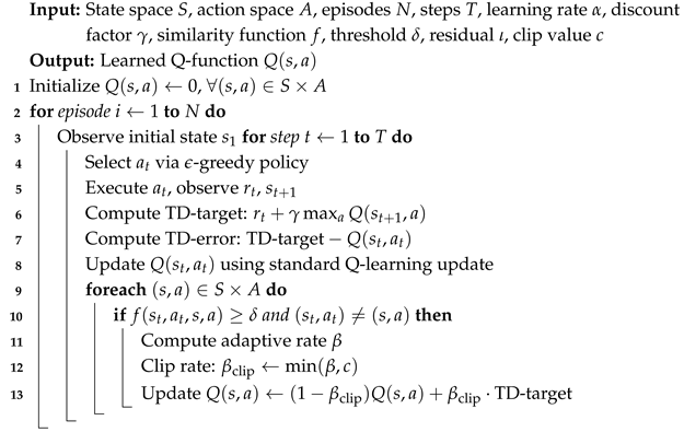
2.1. Q-Learning Algorithm

Q-learning, introduced in [2], is a foundational algorithm in RL. It enables agents to learn optimal action-selection policies within Markov Decision Processes (MDPs) without requiring an environment model.

In an MDP, the agent interacts with an environment composed of states, actions, transition probabilities, and rewards. At each timestep, the agent observes the current state, selects an action, and transitions to a new state according to the environment dynamics. The agent receives a reward based on this transition and aims to learn a policy that maximizes cumulative rewards over time.

An MDP is formally defined by a tuple $(S,A,T,R,\gamma )$, where

• S is the set of states, with $s\in S$ representing a particular state;
• A is the set of actions, with $a\in A$ representing a particular action;
• $T(s,a,s^{\prime })$ is the transition probability function, which gives the probability of transitioning from state s to state $s^{\prime }$ after taking action a;
• $R(s,a,s^{\prime })$ is the reward function, which gives the immediate reward obtained after transitioning from state s to state $s^{\prime }$ due to taking action a;
• $\gamma$ is the discount factor, which determines the importance of future rewards relative to immediate rewards—it is a value between 0 and 1.

The objective in an MDP is typically to find a policy $\pi$, which is a mapping from states to actions, that maximizes the expected cumulative reward over time. This is often formulated as finding the policy that maximizes the expected value of the sum of discounted rewards:

$$V^{\pi }\left(s\right)=\sum _{t=0}^{\infty }{\gamma }^t\mathbb{E}\left[R_{t+1}\right|s_t=s,\pi ]$$

where $V^{\pi }\left(s\right)$ is the value function, representing the expected cumulative reward starting from state s and following policy $\pi$, and $\mathbb{E}\left[R_{t+1}\right|s_t=s,\pi ]$ is the expected immediate reward obtained after taking action a in state s and following policy $\pi$.

The optimal value function $V^{\ast }\left(s\right)$ represents the maximum expected cumulative reward achievable from each state, and the optimal policy ${\pi }^{\ast }\left(s\right)$ is the policy that achieves this maximum expected cumulative reward.

Q-learning maintains an estimate of the value of taking action a in state s, denoted as $Q(s,a)$, which represents the expected cumulative reward the agent will receive if it starts in state s, takes action a, and follows an optimal policy thereafter.

The Q-learning algorithm iteratively updates the Q-values based on the Bellman equation:

$$\begin{array}{cc}\hfill Q(s,a)& \leftarrow Q(s,a)+\alpha \left[R(s,a)+\gamma \underset{a^{\prime }}{max}Q(s^{\prime },a^{\prime })-Q(s,a)\right]\hfill \end{array}$$

where $\alpha$ is the learning rate, controlling the extent to which new information overrides old information, and $s^{\prime }$ is the state reached after taking action a in state s.

The agent interacts with the environment by selecting actions according to an exploration–exploitation strategy, such as $ϵ$-greedy or softmax, to balance between exploring new actions and exploiting the current best-known actions. Over time, as the agent interacts with the environment and receives feedback, Q-learning updates its Q-values to converge toward the optimal action-selection policy, maximizing the cumulative rewards obtained over the agent’s lifetime.

2.2. Similarity-Based Approaches

The ability to use similarity as a means of transferring knowledge is widely recognized in the scientific literature. The use of similarity allows for knowledge generalization, enhances learning efficiency, reduces uncertainty, and promotes cognitive flexibility.

For example, in [9,10], researchers found that humans tend to generalize knowledge learned in specific situations to similar situations, facilitating adaptation to new circumstances. This ability to generalize knowledge is fundamental to human learning and adaptive behavior.

Furthermore, the efficiency of learning through recognizing similarities between past and new situations has been documented in various fields. For instance, in [11], it was highlighted how recognizing similarities enables individuals to quickly grasp and adapt to new situations, resulting in more efficient learning.

The reduction in uncertainty through identifying similarities between situations has also been a subject of research. In [12], it was demonstrated that by identifying similarities, individuals can make informed predictions about future events, allowing them to make decisions with greater confidence and reduce uncertainty associated with the unknown.

Moreover, cognitive flexibility facilitated by the ability to recognize similarities has been extensively studied [13]. This ability enables individuals to easily adapt strategies and approaches used in the past to new circumstances, thereby increasing their ability to solve problems effectively.

This principle is not confined to cognitive sciences but also extends to computational fields such as data mining and supervised learning, where similarity measures play a fundamental role in uncovering hidden patterns [14], clustering [15], classification [16], and handling mixed data [17].

Recent research in RL has also highlighted the significance of similarity in knowledge transfer and adaptation, allowing accelerated learning and improved decision-making in new and unseen environments. RL algorithms, inspired by principles of human learning, utilize similarity to generalize experiences across different states or contexts.

Works like [18,19,20] propose identifying states with similar sub-policies (what could be described by the Principle of Optimality) using homomorphism. These approaches use the history of states, actions, and rewards in a tree-like structure to identify similar sub-policies based on the number of shared items among these sequences, in a model-free fashion. However, these structures and homomorphisms are quite restrictive and computationally expensive [21].

Likewise, there are works such as [22,23,24] that aim to reduce the observation space using an approximation function to represent similitude between states, effectively creating state prototypes. Each prototype contains the most representative features for each subset of similar states. These feature extraction methods are proposed with some adaptation, but they could lead to both good and bad states following the same prototype due to the use of general heuristics and the potential coarseness of the prototype space.

Meanwhile, others [7,8,25] introduce human knowledge directly to abstract the problem’s domain to aid an agent in generalizing its interactions with the environment, decreasing the number of interactions needed to learn. This is achieved by designing a similarity function as a map of states, actions, or state–action pairs to real values between zero and one. These approaches allow the algorithms to obtain ad hoc knowledge for a task, but they also lead to the introduction of biases and other assumptions that the designers may make.

Alternatively, in [25], three categories are defined to help human designers identify similarity in real problems: (1) representational, (2) symmetry, and (3) transition. Representational similarity refers to the generalization of the state–action feature space. Symmetry similarity aims to reduce redundancies for those pairs that are eventually equal given an axis. Transition similarity compares the relative effects of taking an action given a state and where the environment transitions to.

The Q-learning algorithm was upgraded through the integration of representational similarity between elements of the MDP’s two spaces—S for states and A for actions—as proposed by [7]. They state that similarity in these sets could be measured by a norm (though noting this would not always be true or useful in every environment, as [8] remarks). These norms allow some measurement of similarity that is used to select items as "most-likely similar" with a threshold $\parallel s^{\prime }-s_t\parallel \le {\delta }_s$ or $\parallel a^{\prime }-a_t\parallel \le {\delta }_a$. The observed information in Q-learning (the temporal-difference error) is then integrated into these states or actions that are considered similar, as shown in Equation (1), in addition to the normal algorithm behavior. These approaches are denominated as QL-Smooth Observation and QL-Smooth Action, respectively.

$$\begin{array}{cc}\hfill Q(s^{\prime },a)=& Q(s^{\prime },a)+\hfill \\ \hfill & \alpha \left[{\beta }_s\left(r_t+\gamma \underset{a^{\ast }\in A\left(s_t\right)}{max}Q(s_{t+1},a^{\ast })\right)-{\beta }_{s}Q(s^{\prime },a)\right]\hfill \\ \\ \hfill Q(s,a^{\prime })=& Q(s,a^{\prime })+\hfill \\ \hfill & \alpha \left[{\beta }_a\left(r_t+\gamma \underset{a^{\ast }\in A\left(s_t\right)}{max}Q(s_{t+1},a^{\ast })\right)-{\beta }_{a}Q(s,a^{\prime })\right]\hfill \end{array}$$

(1)

Meanwhile, the authors of [8] used a similarity function between states, enabling transitional similarity, denominated as SSAS, with custom similarity functions $\sigma (s_t,a_t,s,a)\mapsto [0,1]$ for all $(s,a)\in S\times A$. They also modified the Q-learning algorithm by integrating this $\sigma$ value, as shown in Equation (2), for each pair whose similarity value is above zero. This algorithm is denominated as QSLearning.

$$\begin{array}{cc}\hfill Q(s^{\prime },a^{\prime })=& Q(s^{\prime },a^{\prime })+\hfill \\ \hfill & \alpha \sigma (s_t,a_t,s^{\prime },a^{\prime })\left[r_t+\gamma \underset{a^{\ast }\in A\left(s_t\right)}{max}Q(s_{t+1},a^{\ast })\right]\hfill \end{array}$$

(2)

Both proposals add a mechanism that uses similarity and performs extra off-policy updates for the same Q-object. QL-smooth uses a norm operation and a threshold to determine which states or actions to update additionally, with a fixed smooth rate $\beta$. The norm measures distance and then chooses a threshold that may disconnect the concept of similarity for some environments and their state–action pairs, while QSLearning updates all pairs available in the MDP where $\sigma >0$, meaning that any positive amount of similarity between state–action pairs is considered sufficient. This could be wasteful and destructive, as the size of $S\times A$ could potentially be large, and allowing $\sigma >0$ for any value to modify the Q-table with Equation (2) with any value of $\alpha$ equates to an excessive number of updates with excessive data.

Nevertheless, these methods have shown good results in their respective applications. Ref. [7] has shown significant speed-up in grid-world tasks and classic control even after a single training episode. And the authors of [8] demonstrated that their algorithm can outperform Q-learning with different designs for $\sigma$ in their corresponding tasks.

At this point, it is relevant to emphasize that the choice of a similarity function is a crucial aspect that must be carefully designed according to the problem domain. Although the effectiveness of similarity-based approaches heavily depends on this measure—since, in the worst case, a poorly chosen metric can compromise results—this characteristic is also one of their key strengths. Their flexible framework allows for an adaptation to diverse problems by leveraging existing similarity measures that naturally fit the context.

In continuous spaces, kernel-based similarities or cosine similarity can be used. For discrete spaces, measures such as exact match or the Jaccard index may be suitable. In geometric problems, position-based metrics are often appropriate. For mixed-data types, integrated functions can combine different approaches: kernel-based similarities (e.g., Gaussian) for continuous features, exact match or set similarity for categorical variables, and embedding-based cosine similarity for textual or image data. An example of this would be a function like $f(s,s^{\prime })=w_{1}Gaussian(s_{pos},s_{pos}^{\prime })+w_{2}ExactMatch(s_{cat},s_{cat}^{\prime })$, where weights $w_1$ and $w_2$ adjust the relative contribution of each component.

Furthermore, when domain-specific knowledge is available, custom similarity functions can be designed. For instance, in robotics, one might combine joint configuration similarity with expected reward metrics. In natural language processing (NLP) tasks, semantic similarity could be integrated with syntactic features to refine outcomes.

2.3. Current Limitations

Despite their demonstrated advantages, existing similarity-based Q-learning approaches exhibit several fundamental limitations that constrain their practical application.

First, computational complexity remains a significant bottleneck. Methods relying on exhaustive similarity searches [20] face $\mathcal{O}\left(\right|S{|}^2)$ time complexity for pairwise state comparisons, becoming prohibitive in large or high-dimensional state spaces. This overhead persists even with approximate similarity metrics, as the comparison operations themselves scale quadratically with the number of states. Moreover, these methods typically lack mechanisms to prioritize or filter updates based on their expected utility or trustworthiness, limiting their scalability.

Second, the static nature of similarity thresholds and update parameters limits adaptability. Approaches like QL-Smooth [7] employ fixed thresholds (${\delta }_s$, ${\delta }_a$) and smoothing factors ($\beta$) that cannot adjust to local variations in state space density or problem dynamics. This rigidity often leads to either insufficient generalization (when thresholds are too strict) or over-propagation of updates (when thresholds are too lenient). Furthermore, such parameters remain constant throughout the learning process, making it difficult to accommodate heterogeneous regions of the state space or evolving dynamics as training progresses.

Third, uncontrolled update propagation risks policy degradation. QSLearning’s [8] strategy of updating all state–action pairs with $\sigma >0$ can introduce harmful interference, particularly when

• The similarity function $\sigma$ imperfectly captures true task-relevant similarities;
• The state–action space contains regions with fundamentally different dynamics;
• The learning rate $\alpha$ remains high during later training stages.

These problems are exacerbated by the fact that existing methods do not incorporate mechanisms to scale updates based on the confidence in value estimates, nor do they adapt similarity propagation in response to learning progress.

Additionally, current methods share two subtle but important weaknesses:

• They lack mechanisms to dynamically adjust similarity measures based on learning progress;
• Their update strategies do not account for the reliability of similarity estimates.

Our XSQ-Learning algorithm, detailed in Section 3, addresses these limitations through three distinctive components: (1) adaptive similarity thresholds that evolve in response to the agent’s current performance and temporal-difference signals, (2) confidence-weighted update propagation that scales similarity-based updates based on the stability of each Q-value estimate, and (3) a local similarity clipping mechanism that limits propagation to highly reliable regions. These design choices maintain the generalization benefits of similarity-based learning while mitigating over-propagation, improving convergence stability, and enhancing scalability to more complex environments.

3. Xperience Similarity-Based Q-Learning (XSQ-Learning)

3.1. Algorithm Overview

The XSQ-Learning algorithm extends traditional Q-learning by incorporating similarity-based value propagation. The core intuition is that state–action pairs with similar expected returns should receive related updates during the learning process. Formally, given a similarity function f that quantifies the relationship between state–action pairs, the algorithm propagates temporal-difference updates proportionally to their pairwise similarity.

This method reflects analogical reasoning principles by transferring learned behaviors across structurally similar experiences. Unlike standard Q-learning which treats each state–action pair in isolation, XSQ-Learning creates a network of related experiences that inform each other’s updates.

3.2. Mathematical Formulation

Let $\mathcal{M}=(S,A,T,R,\gamma )$ be an MDP where

• S is a finite state space;
• A is a finite action space;
• $T:S\times A\times S\to [0, 1]$ is the transition function;
• $R:S\times A\times S\to \mathbb{R}$ is the reward function;
• $\gamma \in [0, 1)$ is the discount factor.

The similarity function $f:{(S\times A)}^2\to [0, 1]$ satisfies

$$f(s,a,s,a)=1\forall (s,a)\in S\times A$$

(3)

$$f(s_t,a_t,s,a)=f(s,a,s_t,a_t)\left(\mathrm{symmetry}\right)$$

(4)

The similarity function can be implemented using various metrics (e.g., cosine similarity for feature vectors, Gaussian kernels for continuous spaces). The specific choice depends on the environment’s characteristics and should reflect meaningful relationships between states.

3.3. Key Components and Pseudocode

1. Adaptive Similarity Thresholding:

$$\mathcal{N}(s_t,a_t)=\{(s,a)\in S\times A\mid f(s_t,a_t,s,a)\ge \delta \}$$

(5)

where $\delta$ dynamically adjusts based on state space density.

The threshold $\delta$ acts as a quality filter, ensuring only sufficiently similar pairs participate in updates. This prevents irrelevant information propagation while maintaining useful generalization.

2. Adaptive rate:

$$\beta =\alpha ·f(s_t,a_t,s,a)·{\displaystyle \frac{\left|\mathrm{TD}-\mathrm{error}\right|}{|\mathrm{TD}-\mathrm{target}-Q(s,a\left)\right|+\iota }}$$

(6)

This triple product ensures that updates are (1) scaled by the learning rate $\alpha$, (2) weighted by similarity, and (3) adjusted according to the relative magnitude of the temporal-difference error. The $\iota$ term prevents division by zero in novel states.

3. Bounded Propagation:

$${\beta }_{\mathrm{clip}}=min(\beta ,\mathrm{sim}\_\mathrm{clip}\_\mathrm{value})$$

(7)

The clip value acts as a safeguard against overly aggressive updates, which are particularly important early in training when Q-value estimates are unreliable.

Algorithm 1 presents the complete XSQ-Learning procedure, which executes three distinct computational phases during each timestep: (i) a conventional Q-learning update for the current state–action pair (lines 7–9); (ii) identification of sufficiently similar state–action pairs through the similarity metric f (line 10); and (iii) propagation of temporal-difference updates weighted by both similarity confidence and error magnitude (lines 11–13). The nested loop structure guarantees exhaustive consideration of all potentially relevant state–action pairs while the similarity threshold $\delta$ preserves computational tractability by limiting updates to only sufficiently similar pairs.

Algorithm 1: XSQ -Learning Algorithm

3.4. Theoretical Analysis

The update rule maintains two key properties:

1. Controlled Update Magnitude:

$$|Q_{t+1}(s,a)-Q_t(s,a)|\le {\beta }_{\mathrm{clip}}·\left|\mathrm{TD}-\mathrm{error}\right|$$

(8)

2. Convergence Guarantee: When $\delta =1$, XSQ-Learning reduces to standard Q-learning, inheriting its convergence properties. For $\delta <1$, convergence is maintained, provided that

$$\sum _{k=1}^{\infty }{\beta }_k=\infty \mathrm{and}\sum _{k=1}^{\infty }{\beta }_k^2<\infty$$

(9)

These conditions ensure that (1) updates continue indefinitely (allowing convergence to optimal values), while (2) update sizes decrease sufficiently to stabilize the learning process. The similarity weighting naturally satisfies these conditions through the $\alpha$ decay.

3.5. Computational Complexity

The algorithm adds $\mathcal{O}\left(\right|S\left|\right|A\left|\right)$ operations per timestep compared to the standard Q-learning’s $\mathcal{O}\left(1\right)$. However, practical implementations can reduce this through

• Locality-sensitive hashing for approximate similarity search;
• Sparse similarity matrices;
• Parallel batch updates.

In large state spaces, computational cost can be managed by (1) pre-computing similarity neighborhoods, (2) using dimensionality reduction on state representations, or (3) implementing selective update strategies that prioritize high-similarity pairs.

3.6. Parameter Selection Guidelines

• $\delta$: Typically initialized to 0.7– 0.9 (higher values enforce stricter similarity) and annealed over time as the agent becomes more confident in its estimates.
• $\iota$: Small constant (${10}^{-5}$) prevents division by zero while being negligible compared to typical TD-error magnitudes.
• c: Upper bounds update magnitude (recommended 0.2–0.5) to maintain stability. Lower values are preferable in highly stochastic environments.

Each parameter contributes to the update process in a specific way: $\delta$ selects which pairs are considered for updates, c restricts the update magnitude, and $\iota$ helps maintain numerical stability. Their optimal values depend on the environment’s reward structure and state space geometry.

4. Experiments and Results

This section presents a comprehensive evaluation of the proposed XSQ-Learning algorithm, comparing its performance against classical Q-Learning and state-of-the-art similarity-based methods: QL-SmoothActions, QL-SmoothObservations, and QSLearning. The experiments measure each algorithm’s efficiency in terms of steps required to achieve the first stable maximum in cumulative reward. All algorithms were tested under identical conditions, including shared parameters (

Table 2. Experimentation parameters.

Parameter	Value	Algorithm
Learn steps	80,000	All
Learning rate $\alpha$	0.1	All
Discount factor $\gamma$	0.99	All
$ϵ$-max	1.0	All
$ϵ$-min	0.25	All
$ϵ$-test	0	All
$ϵ$-life	50,000	All
$ϵ$-schedule	linear decay	All
${\beta }_{\mathrm{smooth}}$	0.2	QL-Smooth Action and Observations
${\beta }_{\mathrm{xsq}}$	0.4	XSQLearning
${\delta }_{\mathrm{s}-\mathrm{action}}$	1.4	QL-Smooth Action
${\delta }_{\mathrm{s}-\mathrm{observation}}$	1.0	QL-Smooth Observation
${\delta }_{\mathrm{xsq}}$	0.8	XSQLearning
$$\sigma (s,s^{\prime })$$	$$\parallel s-s^{\prime }\parallel$$	QL-Smooth Observation
$$\sigma (a,a^{\prime })$$	$$\parallel \exp \_\mathrm{mov}\_dist\left(a\right)-\exp \_\mathrm{mov}\_dist\left(a^{\prime }\right)\parallel$$	QL-Smooth Action
$$\sigma (s,a,s^{\prime },a^{\prime })$$	$${\displaystyle \frac{1}{\left(\sigma (s,s^{\prime })+1\right)\left(\sigma (a,a^{\prime })+1\right)}}$$	XSQLearning, QSLearning

), implementation frameworks, and random seeds. The evaluation uses three progressively complex scenarios in a grid-world environment (Figure 1) to assess scalability and robustness.

4.1. Experimental Setup

The experiments were conducted in a grid-world environment (the implementation of the grid-world environment is available at https://gitlab.com/Bobobert/roddle-env, accessed on 22 June 2025.) (Figure 1) with three scenarios of increasing state space complexity. Scenario 1 serves as the baseline ($cell-size=1$), while Scenarios 2 ($cell-size=2$) and 3 ($cell-size=3$) expand the state space quadratically and cubically, respectively. The environment contains four cell types: open areas (white), obstacles (brown), cliffs (blue), and goals (green). The agent observes only its Cartesian coordinates, and receives rewards of −1 per step and +100 for goal achievement, with episodes limited to 200 steps (reward range: $[-200,100]$). The pink dot in each scenario represents the agent’s starting position.

Each algorithm’s progress was measured in learning steps, where one step equals one environment interaction and Q-model update. Every 500 steps, policies were evaluated over 21 independent test episodes, reporting the mean cumulative reward. To ensure statistical reliability, we ran 20 trials per algorithm with different random seeds. During testing, exploration ($ϵ$) was disabled to evaluate pure exploitation behavior. The following key parameters were standardized: learning rate $\alpha =0.1$ and discount factor $\gamma =0.99$. In contrast, similarity-specific thresholds (e.g., ${\delta }_{\mathrm{xsq}}=0.8$) were tuned per method (Table 2).

4.2. Results and Analysis

The experimental results demonstrate significant performance differences between XSQ-Learning and the comparison algorithms across all three scenarios. Figure 2 illustrates the learning curves. To complement this visual analysis,

Table 3. Mean first stable maximum reward ± standard error over 20 runs.

Algorithm	Scenario 1	Scenario 2	Scenario 3
Q-Learning	93.00 ± 0.00	87.00 ± 0.00	52.85 ± 19.34
QL-SmoothActions	−56.50 ± 32.92	86.00 ± 0.00	80.00 ± 0.00
QL-SmoothObservations	−200.00 ± 0.00	−200.00 ± 0.00	−200.00 ± 0.00
QS-Learning	−200.00 ± 0.00	−200.00 ± 0.00	−200.00 ± 0.00
XSQ-Learning	93.00 ± 0.00	87.00 ± 0.00	80.70 ± 0.11

reports the average value of the first stable maximum reward achieved by each algorithm, along with its standard error, while

Table 4. Mean number of steps to reach the first stable maximum reward ± standard error over 20 runs.

Algorithm	Scenario 1	Scenario 2	Scenario 3
Q-Learning	8150 ± 281.21	27,600 ± 270.48	71,750 ± 858.01
QL-SmoothActions	52,525 ± 6621.68	28,200 ± 2327.86	59,975 ± 534.93
QL-SmoothObservations	80,000 ± 0.00	80,000 ± 0.00	80,000 ± 0.00
QS-Learning	3725 ± 3725.00	2900 ± 2821.35	100 ± 45.88
XSQ-Learning	6650 ± 269.26	19,225 ± 690.61	45,325 ± 826.59

reports the average number of steps to reach the first stable maximum reward achieved by each algorithm, along with its standard error. In parallel,

Table 5. Results comparison all algorithms vs. XSQ-Learning.

Algorithm	Scenario	Average Additional% Steps from $\mathit{XQS}$-$\mathit{Learning}$	Average First Stable Maximum of the Algorithm	Average First Stable Maximum of the $\mathit{XQS}$-$\mathit{Learning}$
Q-Learning	1	22.56	93.00	93.00
QL-SmoothActions		689.85	−56.50	93.00
QL-SmoothObservations		Not Applicable	−200.00	93.00
QS-Learning		Not Applicable	−200.00	93.00
Q-Learning	2	43.56	87.00	87.00
QL-SmoothActions		46.68	86.00	87.00
QL-SmoothObservations		Not Applicable	−200.00	87.00
QS-Learning		Not Applicable	−200.00	87.00
Q-Learning	3	58.30	52.85	80.70
QL-SmoothActions		32.32	80.00	80.70
QL-SmoothObservations		Not Applicable	−200.00	80.70
QS-Learning		Not Applicable	−200.00	80.70

provides quantitative comparisons of convergence speed and stability.

4.2.1. Scenario 1: Baseline Performance

In the simplest environment ($cellsize=1$), both XSQ-Learning and conventional Q-Learning achieved successful policy convergence, though with notable differences in learning efficiency. XSQ-Learning achieved its first stable maximum reward of 93 in an average of 6650 steps, whereas Q-Learning required approximately 22.56% more steps on average (8150 steps) to reach the same outcome. In contrast, the similarity-based variants (QL-SmoothActions, QL-SmoothObservations, and QS-Learning) frequently failed to surpass the minimum reward threshold of −200. Specifically, QL-SmoothActions failed in 10 out of 20 trials, while QL-SmoothObservations and QS-Learning failed in all trials. These results suggest that, in small state spaces, the computational overhead introduced by similarity mechanisms may hinder performance unless carefully controlled, as demonstrated by XSQ-Learning’s adaptive $\delta$ threshold and $sim\_clip\_value$ parameters.

4.2.2. Scenario 2: Moderate Complexity

The quadratic expansion of the state space (cell size = 2) revealed more pronounced advantages for XSQ-Learning. It achieved policy convergence at 87 test points on average (19,225 steps), outperforming Q-Learning, which required 27,600 steps (43.56% more) to reach the same result. Among the similarity-based variants (QL-SmoothActions, QL-SmoothObservations, and QS-Learning) QL-SmoothActions showed the most competitive performance, needing 46.68% more steps than XSQ-Learning to reach an average of 86 test points. Once again, QL-SmoothObservations and QS-Learning failed to achieve meaningful learning, with no successful convergence in any of the 20 trials, highlighting the challenges associated with uncontrolled similarity propagation.

4.2.3. Scenario 3: High Complexity

The cubic expansion of the state space (cell size = 3) resulted in the most pronounced performance differences between XSQ-Learning and Q-Learning. XSQ-Learning reached its first stable maximum reward at an average of 80.70 test points, requiring only 43,525 steps. In contrast, Q-Learning not only failed to match this level of performance—achieving a significantly lower average of 52.85 test points—but also required an average of 71,750 steps to do so, representing 58.30% more steps. Furthermore, in 2 out of 20 trials, Q-Learning did not reach a stable maximum reward at all. Among the remaining similarity-based variants, QL-SmoothActions outperformed Q-Learning in both the reward obtained and the number of steps required. However, compared to the proposed XSQ-Learning, QL-SmoothActions achieved a lower average reward and required 32.32% more steps to converge. Meanwhile, QL-SmoothObservations and QS-Learning completely failed to achieve a stable maximum reward in this scenario, further underscoring the challenges of uncontrolled or misapplied similarity propagation in complex environments.

Notably, the stability of XSQ-Learning was especially evident in this setting: the absence of variance shadows in Figure 2c after convergence indicates highly consistent performance across all random seeds. This strong scalability suggests that XSQ-Learning’s adaptive similarity mechanisms become increasingly effective as the state space grows in size and complexity.

4.2.4. Key Observations

Three principal findings emerge from the experimental results:

• Scaling Advantage: The performance gap between XSQ-Learning and Q-Learning widens with state space complexity. In Scenario 1, the advantage was 22.56%, growing to 43.68% in Scenario 2 and 58.30% in Scenario 3. This demonstrates that XSQ-Learning’s similarity-based updates become increasingly effective as the state space grows.
• Stability: Unlike some similarity-based approaches that showed oscillations or failures, XSQ-Learning maintained consistent performance post-convergence across all scenarios and random seeds. This stability stems from the algorithm’s controlled update propagation through the $sim\_clip\_value$ parameter.
• Robustness: While other similarity-based methods failed completely in certain scenarios (particularly QSLearning), XSQ-Learning demonstrated reliable learning in all test conditions. This robustness comes from the adaptive $\delta$ threshold that automatically adjusts the similarity criteria during learning.

The results suggest that XSQ-Learning alleviates some of the primary challenges noted in previous similarity-based approaches while maintaining the theoretical guarantees of standard Q-learning. The algorithm’s performance advantage is most pronounced in complex environments where traditional methods struggle with slow convergence, making it particularly suitable for real-world applications with large state spaces.

5. Conclusions

In this paper, we proposed XSQ-Learning, a similarity-based RL algorithm designed to improve convergence speed while retaining the stability features of traditional Q-learning methods. Experiments conducted in three increasingly complex environments show that XSQ-Learning outperforms classical and existing similarity-based methods under the tested conditions, with three key contributions emerging from this work:

First, XSQ-Learning addresses fundamental limitations of existing similarity-based methods through its adaptive threshold mechanism ($\delta$) and controlled update propagation ($sim\_clip\_value$). The results in Section 4 show that these innovations successfully prevent the over-generalization and policy degradation observed in methods like QSLearning, while maintaining computational efficiency. In Scenario 3 (the most complex environment), XSQ-Learning reduced the required learning steps by 36.83% compared to standard Q-learning and by 24.43% versus the best similarity-based alternative (QL-SmoothActions).

Second, the results indicate that the algorithm’s performance scales positively with the complexity of the state space. The performance advantage grows linearly with state space complexity—from a 22.56% improvement in Scenario 1 to the substantial 58.30% gain in Scenario 3. This scaling property, combined with the algorithm’s $\mathcal{O}\left(\right|S\left|\right|A\left|\right)$ complexity (Section 3), makes XSQ-Learning particularly suitable for real-world applications where state spaces are typically large and high-dimensional.

Third, post-convergence, XSQ-Learning showed consistent performance across all test scenarios and random seeds (Figure 2). This stability is supported by the use of confidence-weighted updates (Equation (4)) and bounded propagation (Equation 6), which together help reduce interference effects commonly observed in other similarity-based algorithms.

Despite these advantages, we acknowledge that the performance of XSQ-Learning depends on the configuration of three key hyperparameters: the similarity threshold $\delta$, the update clipping value $sim\_clip\_value$, and the residual term $\iota$. While our experiments suggest that effective performance can be achieved within moderate ranges (e.g., $\delta \in [0.7,0.9]$, $sim\_clip\_value\in [0.2,0.5]$, $\iota \approx {10}^{-5}$), it is likely that tuning will be required when deploying the algorithm in new or highly heterogeneous environments. To mitigate this limitation, future research will explore automated hyperparameter optimization techniques such as Bayesian optimization and meta-learning, as well as adaptive scheduling strategies that gradually adjust $\delta$ and $sim\_clip\_value$ during training. These approaches aim to reduce manual tuning effort and enhance the algorithm’s generalizability across tasks.

The findings suggest multiple avenues for future research. First, while our grid-world experiments demonstrate promising results, testing XSQ-Learning in physical systems such as robotic control or autonomous vehicles would validate its practical utility in real-world applications. Second, developing similarity functions capable of effectively handling mixed numerical and categorical state variables would significantly broaden the algorithm’s applicability to more complex, heterogeneous state representations. Third, investigating methods to incorporate catastrophic state avoidance mechanisms during similarity-based updates could enhance the algorithm’s robustness, particularly in safety-critical applications where harmful states must be avoided. Fourth, adapting the principles of XSQ-Learning to function approximation architectures, particularly in deep Reinforcement Learning contexts (e.g., DQN or DDPG), would enable XSQ-Learning to tackle real-world applications with high-dimensional continuous state spaces, such as autonomous robotics and dynamic path planning in uncertain environments

Additionally, relaxing the similarity threshold using linguistic quantifiers—such as “almost all” or “many” objects of the universe—represents a promising avenue to further enhance the flexibility and interpretability of the update mechanism. Formalizing these ideas with intermediate quantifiers, as explored in the literature on fuzzy logic, could provide richer similarity criteria that better handle uncertainty and domain-specific nuances.

The success of XSQ-Learning also raises intriguing theoretical questions about the relationship between state space geometry and learning efficiency. Our results suggest that the algorithm’s performance advantage correlates with the “similarity structure” of the environment—the degree to which nearby states share optimal policies. Formalizing this relationship could lead to new methods for environment characterization and algorithm selection.

In conclusion, XSQ-Learning represents an advance in similarity-based RL, offering practitioners a practical tool for accelerating policy convergence without sacrificing stability. Its empirical performance and theoretical properties suggest potential utility in applications requiring efficient policy convergence.

References

1. Sutton, R.S.; Barto, A.G. Reinforcement Learning: An Introduction; MIT Press: Cambridge, MA, USA, 2018. [Google Scholar]
2. Watkins, C.J.C.H. Learning from Delayed Rewards. Ph.D. Thesis, University of Cambridge, Cambridge, UK, 1989. [Google Scholar]
3. Watkins, C.J.C.H.; Dayan, P. Technical Note: Q-Learning. Mach. Learn. 1992, 8, 279–292. [Google Scholar] [CrossRef]
4. Mnih, V.; Kavukcuoglu, K.; Silver, D.; Rusu, A.A.; Veness, J.; Bellemare, M.G.; Graves, A.; Riedmiller, M.; Fidjeland, A.K.; Ostrovski, G.; et al. Human-level control through deep reinforcement learning. Nature 2015, 518, 529–533. [Google Scholar] [CrossRef] [PubMed]
5. Zhao, H.; Guo, Y.; Liu, Y.; Jin, J. Multirobot unknown environment exploration and obstacle avoidance based on a Voronoi diagram and reinforcement learning. Expert Syst. Appl. 2025, 264, 125900. [Google Scholar] [CrossRef]
6. Zhao, H.; Guo, Y.; Li, X.; Liu, Y.; Jin, J. Hierarchical Control Framework for Path Planning of Mobile Robots in Dynamic Environments Through Global Guidance and Reinforcement Learning. IEEE Internet Things J. 2025, 12, 309–333. [Google Scholar] [CrossRef]
7. Liao, W.; Wei, X.; Lai, J. Smooth Q-learning: Accelerate Convergence of Q-learning Using Similarity. arXiv 2021, arXiv:2106.01134. [Google Scholar] [CrossRef]
8. Rosenfeld, A.; Cohen, M.; Taylor, M.E.; Kraus, S. Leveraging human knowledge in tabular reinforcement learning: A study of human subjects. Knowl. Eng. Rev. 2018, 33, 3823–3830. [Google Scholar] [CrossRef]
9. Gentner, D. Structure-mapping: A theoretical framework for analogy. Cogn. Sci. 1983, 7, 155–170. [Google Scholar] [CrossRef]
10. Gentner, D.; Medina, J. Similarity and the development of rules. Cognition 1998, 65, 263–297. [Google Scholar] [CrossRef] [PubMed]
11. Vlach, H.A.; Sandhofer, C.M. Retrieval dynamics and retention in cross-situational statistical word learning. Cogn. Sci. 2014, 38, 757–774. [Google Scholar] [CrossRef] [PubMed]
12. Kai-Ineman, D.; Tversky, A. Prospect theory: An analysis of decision under risk. Econometrica 1979, 47, 363–391. [Google Scholar] [CrossRef]
13. Raynal, L. Cognitive Flexibility and Analogy; Wiley: Hoboken, NJ, USA, 2022. [Google Scholar] [CrossRef]
14. Rodríguez-González, A.Y.; Aranda, R.; Álvarez Carmona, M.A.; Díaz-Pacheco, A.; Rosas, R.M.V. X-FSPMiner: A Novel Algorithm for Frequent Similar Pattern Mining. ACM Trans. Knowl. Discov. Data 2024, 18, 1–26. [Google Scholar] [CrossRef]
15. Liu, Y.; Ding, J.; Wang, H.; Du, Y. A Clustering Algorithm Based on the Detection of Density Peaks and the Interaction Degree Between Clusters. Appl. Sci. 2025, 15, 3612. [Google Scholar] [CrossRef]
16. Liu, Y.; Zhang, Y.A.; Zeng, M.; Zhao, J. A novel distance measure based on dynamic time warping to improve time series classification. Inf. Sci. 2024, 656, 119921. [Google Scholar] [CrossRef]
17. Grané, A.; Manzi, G.; Salini, S. Dynamic Mixed Data Analysis and Visualization. Entropy 2022, 24, 1399. [Google Scholar] [CrossRef] [PubMed]
18. Girgin, S.; Polat, F.; Alhajj, R. Effectiveness of considering state similarity for reinforcement learning. In Proceedings of the International Conference on Intelligent Data Engineering and Automated Learning, Burgos, Spain, 20–23 September 2006; pp. 163–171. [Google Scholar] [CrossRef]
19. Girgin, S.; Polat, F.; Alhajj, R. State Similarity Based Approach for Improving Performance in RL. IJCAI 2007, 7, 817–822. [Google Scholar]
20. Girgin, S.; Polat, F.; Alhajj, R. Positive impact of state similarity on reinforcement learning performance. IEEE Trans. Syst. Man, Cybern. Part B (Cybernetics) 2007, 37, 1256–1270. [Google Scholar] [CrossRef] [PubMed]
21. Taylor, M.E.; Stone, P. An introduction to intertask transfer for reinforcement learning. Ai Mag. 2011, 32, 15. [Google Scholar] [CrossRef]
22. Li, W.; Meleis, W. Similarity-aware Kanerva coding for on-line reinforcement learning. In Proceedings of the 2nd International Conference on Vision, Image and Signal Processing, Las Vegas, NV, USA, 27–29 August 2018; pp. 1–6. [Google Scholar] [CrossRef]
23. Whiteson, S.; Taylor, M.E.; Stone, P. Adaptive Tile Coding for Value Function Approximation; Technical Report AI-TR-07-339; University of Texas at Austin: Austin, TX, USA, 2007. [Google Scholar]
24. Lin, S.; Wright, R. Evolutionary tile coding: An automated state abstraction algorithm for reinforcement learning. In Proceedings of the Workshops at the Twenty-Fourth AAAI Conference on Artificial Intelligence, Atlanta, GA, USA, 11–12 July 2010. [Google Scholar]
25. Rosenfeld, A.; Taylor, M.E.; Kraus, S. Speeding up tabular reinforcement learning using state-action similarities. In Proceedings of the 16th Conference on Autonomous Agents and MultiAgent Systems, Sao Paulo, Brazil, 8–12 May 2017; pp. 1722–1724. [Google Scholar]
Figure 1. Grid-world scenarios. (a) Scenario 1 ( c e l l s i z e = 1 ). (b) Scenario 2 ( c e l l s i z e = 2 ). (c) Scenario 3 ( c e l l s i z e = 3 ).
Applsci 15 07281 g001
Figure 2. Results from algorithm runs in a grid-world environment. (a) Scenario 1 ( c e l l s i z e = 1 ). (b) Scenario 2 ( c e l l s i z e = 2 ). (c) Scenario 3 ( c e l l s i z e = 3 ). Each shadow corresponds to ±one standard deviation from observed cumulative rewards per episode per seed.
Applsci 15 07281 g002