Article

Modeling and Key Parameter Interaction Analysis for Ship Central Cooling Systems

College of Power Engineering, Naval University of Engineering, Wuhan 430033, China
*
Author to whom correspondence should be addressed.
Appl. Sci. 2025, 15(13), 7241; https://doi.org/10.3390/app15137241 (registering DOI)
Submission received: 7 May 2025 / Revised: 18 June 2025 / Accepted: 18 June 2025 / Published: 27 June 2025
(This article belongs to the Special Issue Nonlinear Dynamics in Mechanical Engineering and Thermal Engineering)

Abstract

To achieve efficient prediction and optimization of the energy consumption of ship central cooling systems, this paper first constructed and validated a high-precision multi-physical domain simulation model of the ship central cooling system based on fluid heat transfer principles and the physical network method. Then, simulation experiments were designed using the Box–Behnken design (BBD) method to study the effects of five key parameters—main engine power, seawater temperature, seawater pump speed, low-temperature fresh water three-way valve opening, and low-temperature fresh water flow rate—on system energy consumption. Based on the simulation data, an energy consumption prediction model was constructed using response surface methodology (RSM). This prediction model exhibited excellent goodness of fit and prediction ability (coefficient of determination R2 = 0.9688, adjusted R2adj = 0.9438, predicted R2pred = 0.8752), with a maximum relative error of only 1.2% compared to the simulation data, confirming its high accuracy. Sensitivity analysis based on this prediction model indicated that main engine power, seawater pump speed, seawater temperature, and three-way valve opening were the dominant single factors affecting energy consumption. Further analysis revealed a significant interaction between main engine power and seawater pump speed. This interaction resulted in non-linear changes in system energy consumption, which were particularly prominent under operating conditions such as high power. This study provides an accurate prediction model and theoretical guidance on the influence patterns of key parameters for the simulation-driven design, operational optimization, and energy saving of ship central cooling systems.

1. Introduction

Under the dual pressures of continuously growing global energy demand and increasingly stringent environmental regulations, improving energy efficiency and controlling emissions from ships, as key transportation tools, have become a central focus for the industry [1,2,3]. The ship’s central cooling system is not only a core auxiliary system ensuring the stable operation of the power plant, but its operational energy consumption also constitutes a significant portion of the ship’s total energy consumption [4,5,6]. Therefore, in-depth research and the establishment of accurate energy consumption prediction models for the ship’s central cooling system are of crucial importance and practical value for effectively evaluating energy efficiency levels, exploring energy-saving potential, and optimizing operational management.
Existing research widely suggests that applying variable speed drive (VSD/VFD) technology can significantly improve the energy efficiency and operational efficiency of ship cooling systems. For instance, analysis by Kocak et al. [5] indicates that VSD/VFD technology, by effectively adjusting pump speed according to cooling demand, can significantly reduce energy consumption and enhance system efficiency while meeting operating requirements. Research by Su et al. [7] also confirms this point and further emphasizes the technology’s good adaptability under varying operating conditions. However, it is noteworthy that the energy-saving potential of VSD/VFD technology is not always automatically realized; its full benefit realization heavily relies on advanced control strategies and precise system adjustment. Addressing this, Jeon et al. [8] focused on ship central freshwater cooling systems, and to further enhance their energy efficiency control level, they proposed and validated an optimized control scheme using a merchant marine training vessel as a platform. Their study first deeply analyzed the existing system, identified key areas for energy efficiency improvement, and consequently designed an improved control strategy. Subsequent sea trial results demonstrated that the scheme can effectively reduce the energy consumption of cooling water pumps and significantly improve the overall operational efficiency of the system. To better guide such optimization practices and accurately evaluate their benefits, Pariotis et al. [9] developed a model-based method specifically for assessing the energy-saving potential of seawater pumps after adopting VSD/VFD technology. This research successfully achieved a quantitative assessment of energy efficiency improvement before and after the technological modification by integrating system-level modeling with actual operating data, thereby providing strong theoretical support for optimizing VSD pump operation strategies and designing more energy-efficient solutions. Similarly, in the field of general pump systems, Yimchoy et al. [10] also developed a modeling and simulation-based VFD energy efficiency assessment method. This method, by comparatively analyzing the energy consumption differences between VFD and constant speed pumps under different operating conditions, provided valuable reference for quantifying the energy-saving potential of VFD in various pump applications, including ship cooling systems, and for their optimized configuration. Furthermore, the precise control achieved through VSD/VFD technology not only yielded significant energy savings but also helped reduce equipment wear, which can potentially lead to reduced maintenance costs and ultimately enhance the overall reliability of the system [11]. The advantage of VSD/VFD technology in adapting to different operating conditions is particularly prominent. For instance, studies by Dere et al. [12] and Theotokatos et al. [13] both indicate that, especially under low load conditions such as slow steaming, dynamically adjusting the pump load can effectively reduce unnecessary energy losses, further highlighting the critical role played by optimized control strategies in achieving multi-condition energy efficiency improvement.
Currently, researchers commonly analyze and optimize the energy efficiency and operational efficiency of systems by applying variable speed drive (VSD/VFD) technology or by adjusting operating parameters based on specific working conditions. These studies undoubtedly lay an important theoretical foundation and provide valuable engineering guidance for the design selection and overall performance optimization of ship cooling systems. However, a ship cooling system is essentially a complex coupled system involving multiple physical fields and transient processes, whose energy consumption is influenced by the combined effects of various operating parameters and environmental factors [14,15]. Solely relying on VSD/VFD for the speed regulation of a single piece of equipment, or adjusting individual parameters based on simplified assumptions, often struggles to fully address the intricate dynamic coupling effects and interactions among multiple factors in actual operation. This, to some extent, limits the potential for the system to achieve globally optimal energy efficiency. Simultaneously, these methods often find it difficult to accurately capture the nuances of all key factors and their mutual influences, leading to potentially limited optimization effects or effects that are only evident under specific operating conditions. Furthermore, gaining a deep understanding of these complex interactions through traditional multi-physical field coupled simulation modeling is not only inherently challenging but also computationally intensive and time-consuming. Conversely, conducting comprehensive experimental studies is often constrained by high costs and demanding implementation conditions. Therefore, there is an urgent need for a new modeling approach that can efficiently reveal how key factors and their interactions affect system performance. Response surface methodology (RSM) is precisely such a powerful statistical modeling technique. Leveraging optimized experimental design, it can efficiently construct mathematical models of the relationship between input parameters and system responses using relatively few data points. Such models not only clearly reveal the influence patterns of individual parameters and their interactions on the system response, making them particularly suitable for analyzing highly coupled multi-parameter problems like ship cooling systems, but their modeling process is also relatively fast, and the resulting predictive models demonstrate excellent computational efficiency. The core objective of RSM is to obtain an empirical model with good predictive accuracy at a reasonable experimental or simulation cost, thereby providing an efficient tool for in-depth analysis, accurate prediction, and effective optimization of the system [16,17,18].
To accurately predict the energy consumption of ship central cooling systems and gain a deep understanding of the influence of key operating parameters on system performance, this paper focused on the central cooling system of a certain type of bulk carrier. The research employed a combined approach of numerical simulation and experimental design. First, based on the multi-physical domain modeling technique, a dynamic simulation model of the system was constructed and validated using actual ship data. Secondly, using this model and the experimental design method, the influence patterns of several key operating parameters on system energy consumption were systematically investigated. Furthermore, a high-precision energy consumption prediction model was developed using response surface methodology, and this model was utilized to analyze the influence mechanism of main parameters and their interactions on system energy consumption, revealing its nonlinear characteristics. This paper aimed to provide a reliable prediction tool and theoretical guidance for the performance evaluation, energy consumption characteristics analysis, operation optimization, and the development of energy-saving strategies for ship central cooling systems.

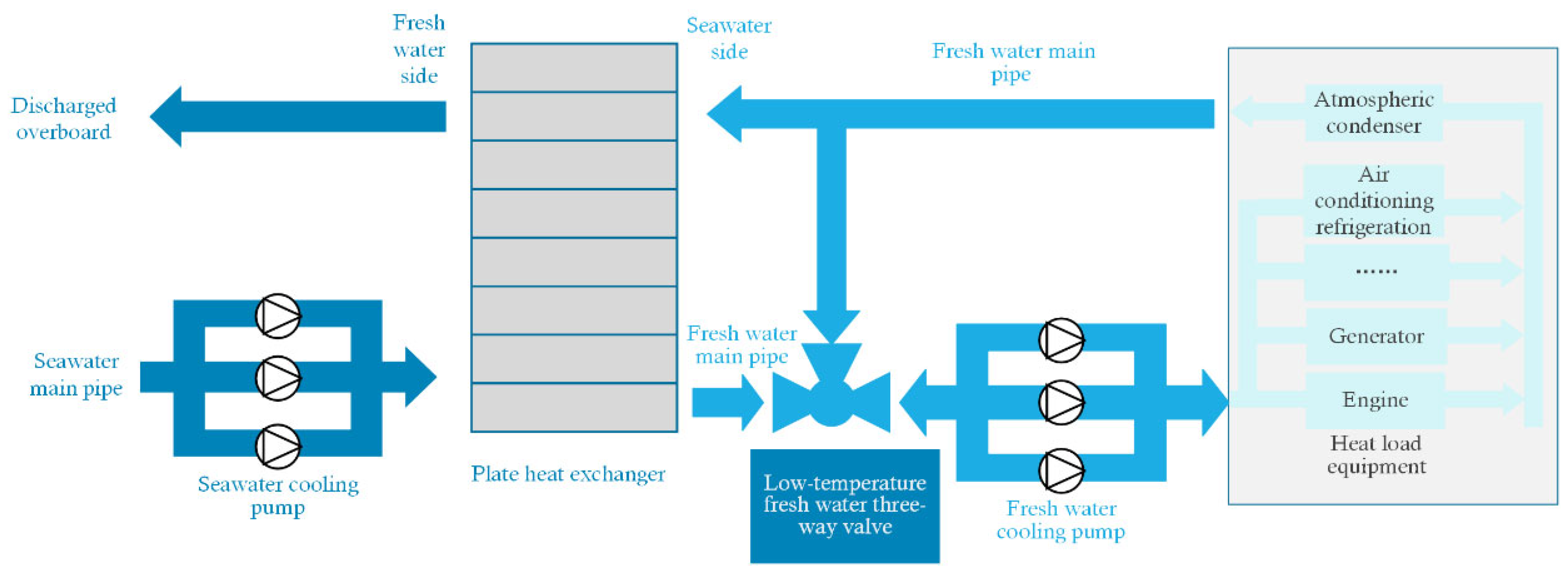
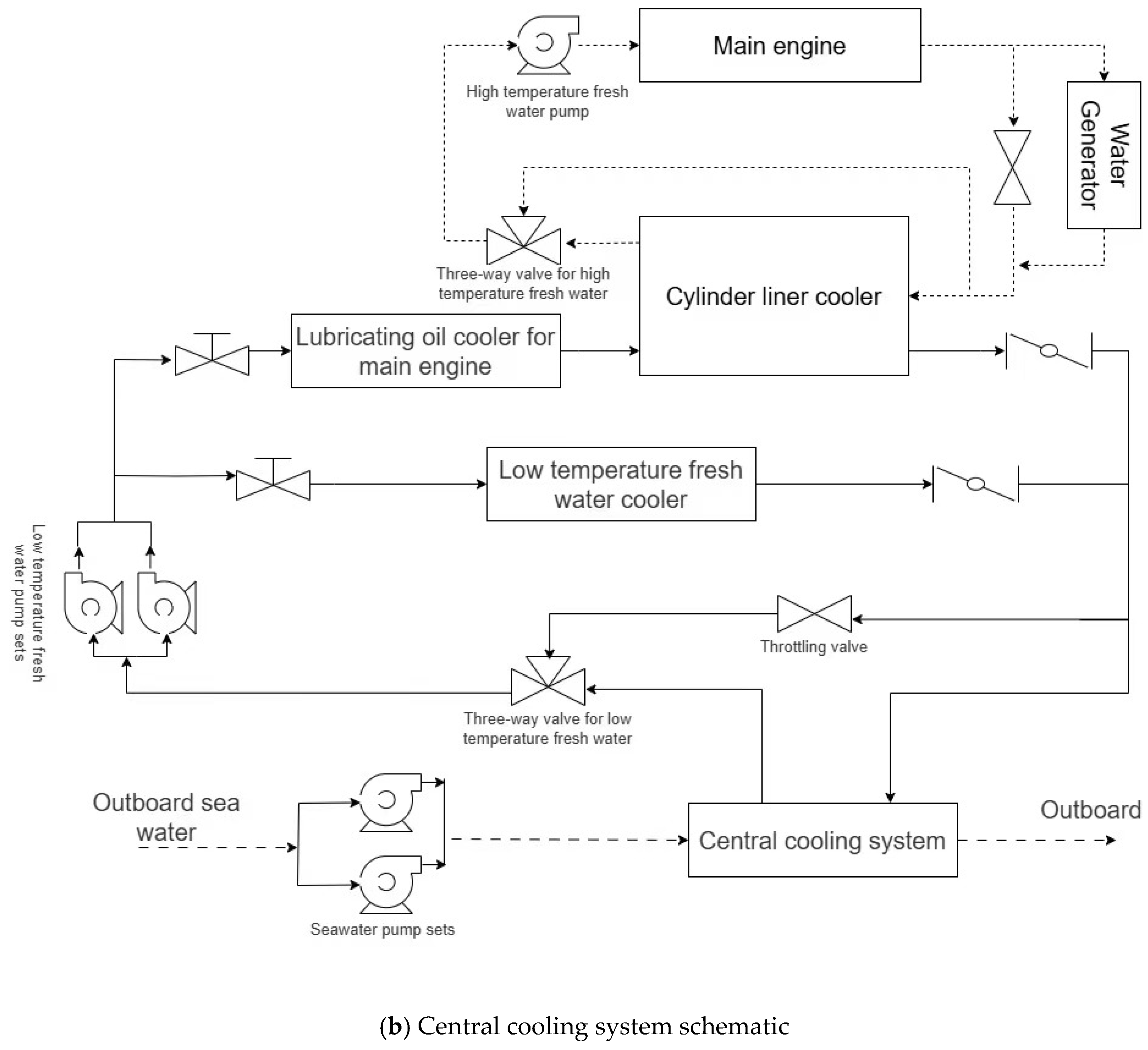
2. Principle of Operation of the Ship Central Cooling System

This paper used the central cooling system of a certain type of bulk carrier as the research object. In this system, low-temperature fresh water, cooled by the central cooler, is regulated by the low-temperature fresh water three-way valve (hereinafter referred to as the “three-way valve”) to precisely control its temperature at 36 °C. Subsequently, the low-temperature fresh water is transported by the cooling pump to various heat load equipment for heat exchange and finally returns to the central cooler to complete the cooling cycle (Figure 1).

3. Calculation Model

3.1. Mathematical Model

The total power consumption of the central cooling system consisted of the power consumption of the system’s seawater pumps and fresh water pumps. Based on the principle of energy conservation, the shaft power of a single pump is expressed by Formula (1) [4]:
P p = ρ · g · Q · H 3.6 × 10 6 η
where P p is the shaft power of a single pump, in kW; ρ is the fluid density (seawater or fresh water), in kg/m3; g is the acceleration due to gravity, in m/s2; Q is the seawater or fresh water flow rate, in m3/h; H is the pump head, in m; and η is the pump efficiency.
The total power consumption of the system was the sum of the shaft powers of all relevant pumps, as shown in Formula (2):
P _ t o t a l = i = 1 n P_ ( p , i )
where P_ t o t a l is the total power consumption of the system, in kW; P_ ( p , i ) is the shaft power of the ith pump, in kW; and n is the total number of seawater and fresh water pumps in the system.
The pressure loss in the system’s piping consisted of frictional losses along the length and local losses. The frictional loss along the length is calculated according to Formula (3):
h f = λ L d · v 2 2 g
where h f is the frictional loss along the length, in m; λ is the friction resistance coefficient; L is the pipe length, in m; d is the internal diameter of the pipe, in m; v is the flow velocity, in m/s; and g is the gravitational acceleration, in m/s2.
Local resistance loss was generated when fluid flowed through pipe fittings (such as elbows, valves, etc.) and can be calculated using Formula (4):
h a = ξ v 2 2 g
where h a is the local resistance loss, in m; ξ is the local resistance coefficient; and v is the flow velocity, in m/s.
The total resistance loss was the pressure loss from both the pipeline and fittings and can be expressed as Formula (5):
Δ H = h f + h a
where Δ H is the total head loss, in m.
To accurately describe the heat transfer process of the system, the main heat balance governing equation was established, as shown in Formula (6):
Q = m c p ( T i n T o u t )
where Q is the heat transfer rate, in kW; m is the mass flow rate of the cooling medium, in kg/s; c p is the specific heat capacity of the cooling medium at constant pressure, in kJ/(kg·K); T i n is the inlet temperature of the cooling medium, in °C; and T o u t is the outlet temperature of the cooling medium, in °C.
The calculation formula for the flow characteristics of a three-way valve is shown in Formula (7):
Q = K · ( V V m a x ) α
where Q is the flow rate, in m3/s; K is the flow coefficient; V is the valve opening; V m a x is the maximum flow rate, in m3/s; and α is the opening exponent, dimensionless, reflecting the relationship between the valve flow rate and opening.
Detailed calculations of pressure drop in the equipment, pump head calculations, and the specific characteristics of the three-way valve were all based on standard fluid dynamics principles and equipment specifications. Specific details can be found in the cited literature [19].

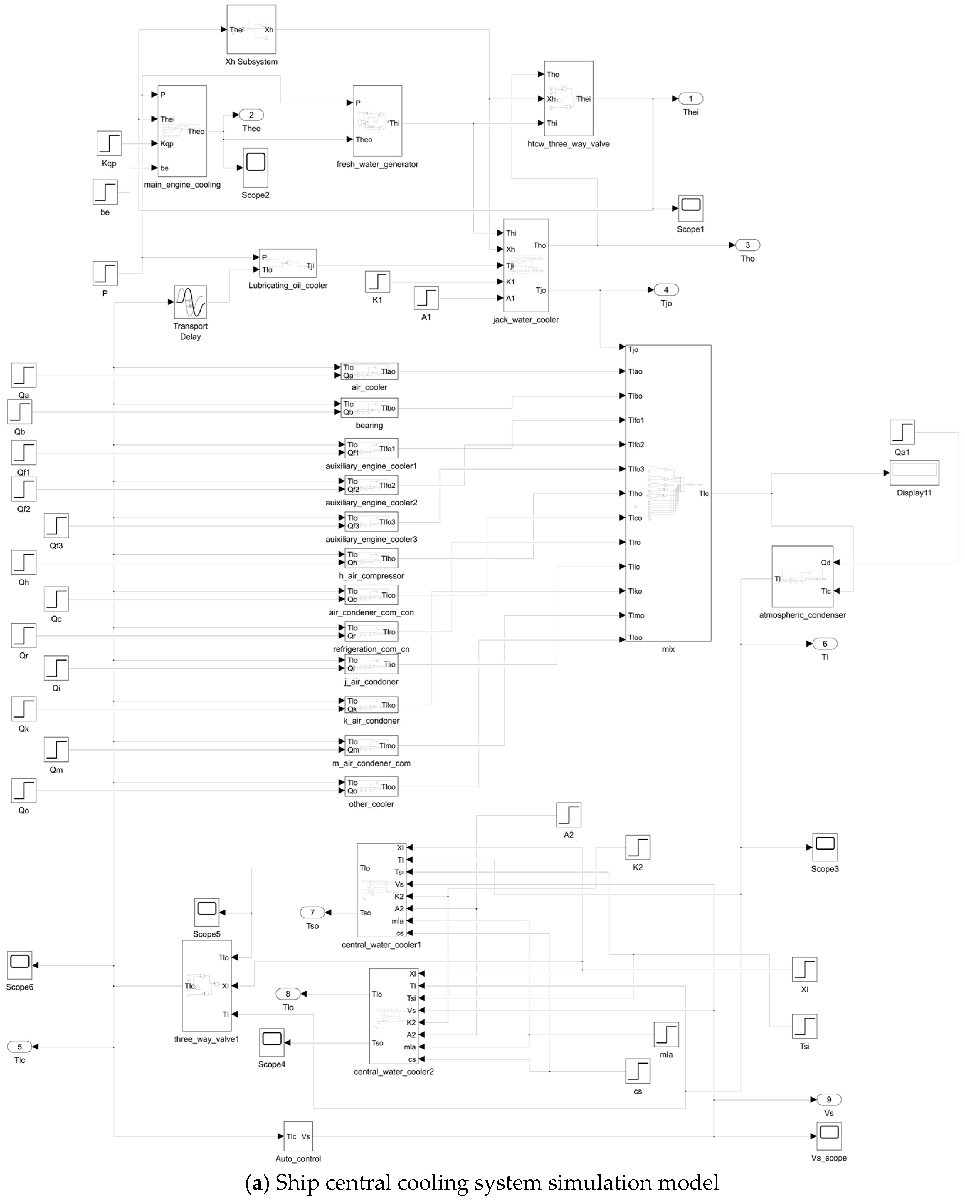
3.2. Establishment of the Simulation Model

In this paper, the central cooling system of a certain type of ship was taken as the research object, and its dynamic simulation model was established in the Simulink environment using the physical network method. The basic parameters for the model’s design service speed (100% load) operating condition are detailed in Table 1. The simulation system consisted of a mutually coupled high-temperature fresh water loop, low-temperature fresh water loop, and seawater loop. The high-temperature fresh water loop model mainly included the main engine jacket water heat load model, high-temperature fresh water cooler model, fresh water generator model, and dynamic model of the high-temperature fresh water three-way valve (diverting/mixing). The low-temperature fresh water loop model integrated models of key components, such as the central cooler, main engine air cooler, main engine lubricating oil cooler, low-temperature fresh water diverting three-way valve, and other auxiliary cooling equipment. The seawater loop model mainly included the seawater pump model, central cooler (seawater side) model, piping model, etc. The overall structure of the constructed central cooling system Simulink simulation model is shown in Figure 2.

3.3. Simulation Model Validation

To validate the accuracy of the simulation model, actual ship design condition data were input into the model for simulation [19]. Table 2 compares the simulation results with the actual ship design values. The results showed that the relative errors of the main system parameters were all less than 2%, which validated that the simulation model had good accuracy.

4. Development of the Response Surface Model

4.1. Selection of Design Variables

In order to develop a response surface model (RSM) capable of accurately predicting the energy consumption of the ship’s central cooling system and revealing parameter interactions, based on the preceding calculation model, this paper selected the following five parameters as design variables: main engine power, seawater temperature, seawater pump speed, opening of the low-temperature loop three-way control valve, and low-temperature freshwater flow rate. The selection of these parameters aimed to cover key aspects such as the main heat load source, external cooling conditions, core energy consumption units, and critical links in internal heat distribution and control while simultaneously providing a basis for the subsequent analysis of the influence of each parameter and their interactions on total energy consumption.

4.2. Principle and Modeling of Response Surface Methodology

Response surface methodology (RSM) is an optimization technique combining mathematical and statistical methods, widely applied in studies exploring the relationship between multiple input variables (factors) and one or more output variables (responses). Its core idea is to obtain data through systematic design of experiments (DoE), construct a mathematical model (typically a polynomial model) to approximate the true response surface within the factor space, and subsequently analyze the influence of each factor and their interactions on the response, ultimately finding the optimal combination of factor levels or understanding the key influencing factors of the process [16].
Considering the multi-parameter interactive effects within the multi-physical fields of the ship’s central cooling system and simultaneously balancing fitting accuracy and computational efficiency, this paper selected a quadratic polynomial model to construct the energy consumption response surface. This model can effectively capture the surface curvature characteristics and the interaction effects between factors while achieving a balance between fitting accuracy and computational efficiency. Its general mathematical expression is [20]:
y = β 0 + i = 1 k β i x i + i = 1 k β i i x i 2 + i < j k β i j x i x j + ε
where y is the response value, β0 is the constant term, βi and βij are the regression coefficients, xi and xj are the factor levels, and ε is the error term; k is the number of factors, which is 5 in this paper.

4.3. Box–Behnken Experimental Design

Based on the typical non-linear relationships and potential interactive effects among the parameters of the ship’s central cooling system, the complexity of accurately predicting system energy consumption was significantly increased. To effectively capture these complex second-order effects and parameter interactions, this paper employed the Box–Behnken design (BBD) from response surface methodology (RSM) for experimental design [21] (schematic diagram shown in Figure 3). As an efficient three-level, second-order design method, BBD can construct predictive models containing quadratic and interaction terms with relatively fewer experimental runs. For the five key independent variables (factors) focused on in this study (see Table 3), BBD required only 46 runs to comprehensively analyze the influence of the main effects and interaction effects of each factor on energy consumption, significantly improving the efficiency of experimental design and data analysis and laying the foundation for the refined modeling of system energy consumption.
Following the principles of Box–Behnken design, the five factors influencing the central cooling system’s energy consumption, namely main engine power, seawater temperature, seawater pump speed, three-way valve opening, and low-temperature fresh water flow rate, were selected as the independent variables for the experiment, denoted as X1, X2, X3, X4, and X5, respectively. System energy consumption F was taken as the dependent variable for this experiment. The five independent variables were set at three levels each, coded as −1, 0, and +1, representing the low, medium, and high levels for each factor, respectively. An experimental plan was formulated based on this.

4.4. Establishment of the Response Prediction Model

A multiple quadratic regression prediction model for the central cooling system’s energy consumption was obtained by fitting using the least squares method. The expression is given by Equation (9):
F ( X ) = 87.91 + 18.68 X 1 + 4.52 X 2 + 5.98 X 3 + 3.19 X 4 + 1.31 X 5 3.80 X 1 X 2 + 6.15 X 1 X 3 1.14 X 1 X 4 0.4 X 1 X 5 X 2 X 3 1.14 X 2 X 4 + 0.275 X 3 X 4 + 1.06 X 3 X 5 + 1.31 X 4 X 5 + 7.46 X 1 2 0.9619 X 2 2 2.45 X 3 2 + 0.944 X 4 2 0.7944 X 5 2
where F(X) is the energy consumption of the ship’s central cooling system, in N; X1 is the main engine power, in kW; X2 is the seawater temperature, in °C; X3 is the seawater pump speed, in rpm; X4 is the three-way valve opening; and X5 is the low-temperature fresh water flow rate, in m3/s.

5. Results and Analysis

5.1. Analysis of Variance for the Model

Analysis of variance for the established model and significance tests for the model and regression coefficients were performed, as shown in Table 4.
From the analysis of variance in Table 3, it can be seen that the model significance test yielded p < 0.0001, indicating that the regression prediction model was significant. The F-value of 10.94 further confirmed the overall significance of the model. The residual sum of squares for the model was 873.71, with 25 degrees of freedom, and the mean squared error was 34.95. These metrics indicated a good fit of the model to the data and its ability to effectively capture the variability in the data. Therefore, this model can be reliably used to analyze the influence of various factors on the energy consumption of the ship’s central cooling system.

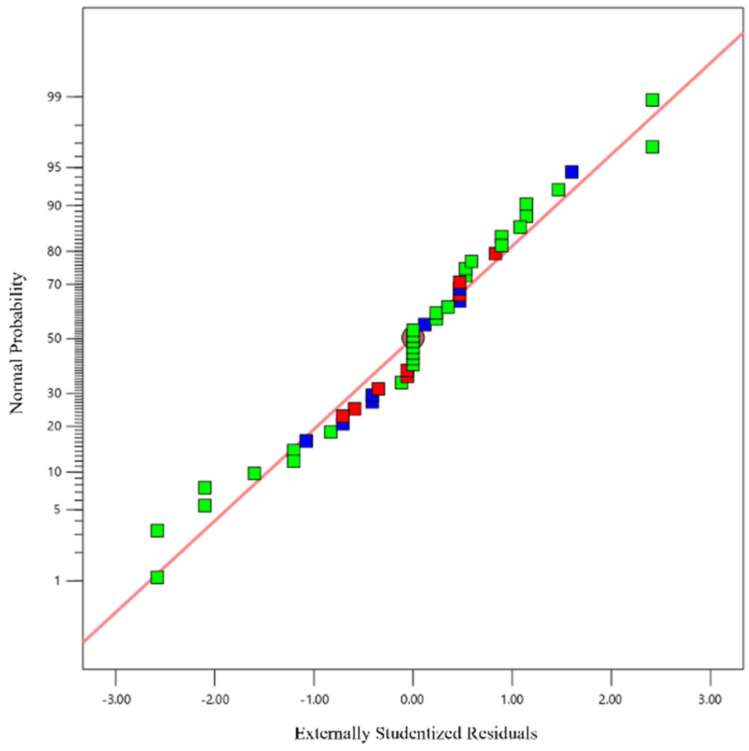
5.2. Model Evaluation

(1) Coefficient of Determination R 2
R 2 = 1 S S E S S T
R 2 a d j = 1 S S E / d E S S T / d T = 1 d T d E ( 1 R 2 )
R p r e d 2 = 1 P R E S S S S T
where SSE represents the sum of squares of error; SSM represents the model sum of squares; SST represents the total sum of squares; dE represents the degrees of freedom for the sum of squares of error; dT represents the degrees of freedom for the total sum of squares; and PRESS represents the predicted residual sum of squares.
The effective range for the values of the three evaluation metrics was between 0 and 1. A value closer to 1 for R2, R2adj, and R2pred indicated a better model fit.
From Table 5, it can be seen that in this regression, R2 = 0.9688, indicating that 96.88% of the variability in the dependent variable was explained by the model. R2adj = 0.9438, indicating that the constructed response surface model can explain 94.38% of the variability in the response values, adjusted for the number of predictors. The difference between R2 and R2adj was only 0.025 (0.9688–0.9438), which was small, suggesting a good model fit. R2pred = 0.8752. The difference between R2pred and R2adj was 0.0686 (0.9438–0.8752), indicating that the model had good predictive ability. Therefore, the response surface model constructed in this experiment demonstrated good predictive performance and can be effectively used for predicting and analyzing the experimental data.
(2) Residual Normal Probability Plot
The residual normal probability plot was used to assess the normality of the residuals. As shown in Figure 4, most of the experimental points (blue points) are closely distributed along the regression line, with only a few potential outliers (red points) deviating from it. Overall, this indicates that the model has good accuracy.

5.3. Prediction Model Validation

To validate the established model, five sets of data were randomly selected within the parameter ranges. Table 6 shows a comparison of the energy consumption predicted by the regression model and the numerical simulation results. The maximum error was 1.2%, indicating the accuracy of the prediction model.

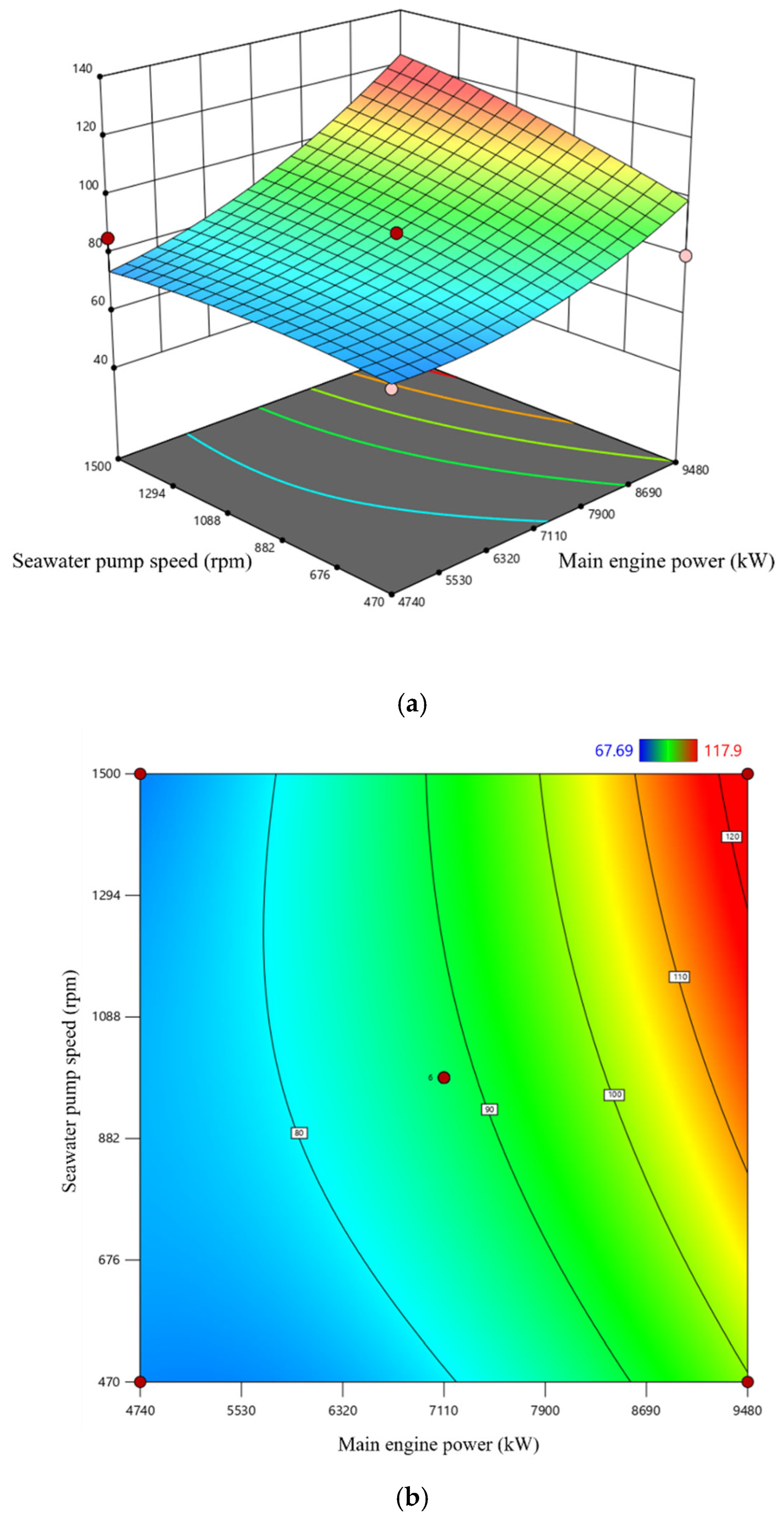
5.4. Analysis of Key Parameter Sensitivity and Interaction

As shown in Table 3, by observing the F-values of each factor, it can be inferred that main engine power, seawater pump speed, seawater temperature, and three-way valve opening had relatively significant effects on system energy consumption. The degree of impact of these important factors on system energy consumption was as follows: main engine power (X1) > seawater pump speed (X3) > seawater temperature (X2) > three-way valve opening (X4). Notably, the F-value for main engine power (X1) was considerably larger than those of the other influencing factors, indicating its dominant impact on the energy consumption of the ship’s central cooling system. Given that seawater pump speed (X3) was the most critical adjustable operating parameter among these, and its optimal setting was dependent upon varying load (X1) and seawater temperature (X2), implementing precise variable frequency control for the seawater pump, tailored to the load and ambient temperature, represented a core and effective strategy for unlocking the energy-saving potential of this system. Furthermore, the three-way valve opening (X4) should be synergistically optimized in accordance with the actual operating conditions to achieve optimal overall system energy performance.
Figure 5a and Figure 5b respectively present the response surface and contour plots illustrating the interaction effect of main engine power (X1) and seawater pump speed (X3) on system energy consumption. The curvature, gradient of the response surface, and the shape and distribution density of the contour lines intuitively reflected the main effects and interaction strength of each factor. As shown in Figure 5a, the response surface exhibited a steep increasing gradient along the main engine power (X1) axis, indicating that within the studied range, X1 was the dominant factor influencing system energy consumption, and its increase will lead to a significant rise in energy consumption. Along the seawater pump speed (X3) axis, the response surface also showed an increasing trend, but with a relatively gentle gradient, suggesting that while seawater pump speed directly impacted energy consumption, its main effect strength was much weaker than that of the main engine power. From a physical mechanism perspective, the increase in main engine power directly determined the thermal load the system needed to dissipate, which was the primary cause of increased cooling demand and energy consumption. In contrast, an increase in seawater pump speed directly raised the pump’s own operating power and the fluid’s resistance loss in the pipeline, thereby jointly increasing the total system energy consumption. It is worth noting that when the main engine power was in the higher range, the gradient of the response surface along the seawater pump speed (X3) axis significantly increased. This indicates that under high load operating conditions, the system’s energy consumption becomes highly sensitive to changes in seawater pump speed.
The contour plot in Figure 5b shows that the contour lines exhibited a distinct elliptical or curved shape, rather than nearly parallel straight lines, revealing a relatively significant interaction between main engine power (X1) and seawater pump speed (X3). This interaction implied that the effects of the two factors on energy consumption were not simply linearly additive but rather involved a synergistic effect. Specifically, when both main engine power and seawater pump speed were simultaneously at high levels, the system faced the dual pressures of increased thermal load and sharply increased pump power consumption, leading to a non-linear accelerated growth trend in total system energy consumption. This highlights the necessity of collaborative optimal control under such operating conditions. Therefore, by developing intelligent control strategies that dynamically optimize and set the seawater pump speed based on real-time main engine power, the non-linear surge in energy consumption in high-load regions can be precisely avoided.

6. Conclusions

(1) This study constructed physical models of core components and established a multi-physical domain simulation system using the physical network method, successfully developing an energy consumption prediction model for the ship’s central cooling system. The model effectively captured the complex nonlinear relationships and interactions among multiple factors. Model performance evaluation demonstrated excellent goodness-of-fit and predictive capability: the coefficient of determination R2 = 0.9688, adjusted R2adj = 0.9438, and predicted R2pred = 0.8752. Numerical test validation showed a maximum relative error of only 1.2%, further confirming the model’s high prediction accuracy and practical application potential.
(2) Sensitivity analysis of the ship’s central cooling system energy consumption prediction model revealed that main engine power, seawater pump speed, seawater temperature, and three-way valve opening were the significant single factors affecting the system’s energy consumption and had the greatest impact on its energy-saving potential. Therefore, implementing variable frequency precision control for the seawater pump based on load and ambient temperature is the core strategy for achieving energy savings in this system. Meanwhile, the three-way valve opening must be synergistically optimized to achieve optimal overall system energy efficiency.
(3) Based on the Box–Behnken design (BBD) response surface method and focusing on five key factors—main engine power, seawater temperature, seawater pump speed, three-way valve opening, and low-temperature fresh water flow rate—this study further clarified the influence of interaction effects among these factors on system energy consumption. Analysis revealed a significant interaction between main engine power and seawater pump speed, where their synergistic effect led to a nonlinear increase in system energy consumption, which was particularly prominent at high power. In-depth analysis of this interaction mechanism provided a crucial basis and new perspectives for developing collaborative optimization control strategies to further reduce the ship’s central cooling system energy consumption.

Author Contributions

Conceptualization, X.W.; Methodology, X.W.; Software, P.S.; Validation, P.Z.; Investigation, X.W. and J.W.; Resources, P.S.; Data curation, P.Z.; Writing—original draft, X.W.; Writing—review & editing, P.Z. and J.W.; Visualization, P.S.; Funding acquisition, P.Z. All authors have read and agreed to the published version of the manuscript.

Funding

This research and the APC were funded by the Independent Project of the Naval University of Engineering (2023502080).

Institutional Review Board Statement

Not applicable.

Informed Consent Statement

Not applicable.

Data Availability Statement

The original contributions presented in this study are included in the article. Further inquiries can be directed to the corresponding author.

Conflicts of Interest

The authors declare no conflict of interest.

References

  1. Jimenez, V.J.; Kim, H.; Munim, Z.H. A review of ship energy efficiency research and directions towards emission reduction in the maritime industry. J. Clean. Prod. 2022, 366, 132888. [Google Scholar] [CrossRef]
  2. Wang, K.; Wang, J.; Huang, L.; Yuan, Y.; Wu, G.; Xing, H. A comprehensive review on the prediction of ship energy consumption and pollution gas emissions. Ocean Eng. 2022, 266, 112826. [Google Scholar] [CrossRef]
  3. Fan, A.; Yan, J.; Xiong, Y.; Shu, Y.; Fan, X.; Wang, Y.; He, Y.; Chen, J. Characteristics of real-world ship energy consumption and emissions based on onboard testing. Mar. Pollut. Bull. 2023, 194, 115411. [Google Scholar] [CrossRef] [PubMed]
  4. Jeon, T.-Y.; Jung, B.-G. A Study of PI Controller Tuning Methods Using the Internal Model Control Guide for a Ship Central Cooling System as a Multi-Input, Single-Output System. J. Mar. Sci. Eng. 2023, 11, 2025. [Google Scholar] [CrossRef]
  5. Kocak, G.; Durmusoglu, Y. Energy efficiency analysis of a ship’s central cooling system using variable speed pump. J. Mar. Eng. Technol. 2018, 17, 43–51. [Google Scholar] [CrossRef]
  6. Jeon, T.Y.; Lee, Y.C. Energy saving in ship central cooling systems: IMC-Tuned PID with feedforward control. J. Mar. Sci. Eng. 2025, 13, 510. [Google Scholar] [CrossRef]
  7. Su, C.L.; Chung, W.L.; Yu, K.T. An energy-savings evaluation method for variable-frequency-drive applications on ship central cooling systems. IEEE Trans. Ind. Appl. 2014, 50, 1286–1294. [Google Scholar] [CrossRef]
  8. Jeon, T.-Y.; Lee, C.-M.; Hur, J.-J. A study on the control solution of ship’s central fresh water-cooling system for efficient energy control based on merchant training ship. J. Mar. Sci. Eng. 2022, 10, 679. [Google Scholar] [CrossRef]
  9. Pariotis, E.; Zannis, T.; Katsanis, J.S. An integrated approach for the assessment of central cooling retrofit using variable speed drive pump in marine applications. J. Mar. Sci. Eng. 2019, 7, 253. [Google Scholar] [CrossRef]
  10. Yimchoy, S.; Supatti, U. An energy-savings evaluation method for variable-frequency-drive applications on water pump systems. In Proceedings of the 2021 24th International Conference on Electrical Machines and Systems (ICEMS), Gyeongju, Republic of Korea, 31 October–3 November 2021; pp. 603–608. [Google Scholar] [CrossRef]
  11. Lee, C.M.; Jeon, T.-Y.; Jung, B.-G.; Lee, Y.-C. Design of energy saving controllers for central cooling water systems. J. Mar. Sci. Eng. 2021, 9, 513. [Google Scholar] [CrossRef]
  12. Dere, C.; Deniz, C. Load optimization of central cooling system pumps of a container ship for the slow steaming conditions to enhance the energy efficiency. J. Clean. Prod. 2019, 222, 206–217. [Google Scholar] [CrossRef]
  13. Theotokatos, G.; Sfakianakis, K.; Vassalos, D. Investigation of ship cooling system operation for improving energy efficiency. J. Mar. Sci. Technol. 2017, 22, 38–50. [Google Scholar] [CrossRef]
  14. Meyers, W.T. Design, Analysis and Modeling of a Modular Navy Integrated Power and Energy Corridor Cooling System; Massachusetts Institute of Technology: Cambridge, MA, USA, 2024. [Google Scholar]
  15. Wang, J.; Zhao, F.; Sun, L.; Hou, Y.; Chen, N. Research on the energy savings of ships’ water cooling pump motors based on direct torque control. Processes 2023, 11, 1938. [Google Scholar] [CrossRef]
  16. Chi, G.; Hu, S.; Yang, Y.; Chen, T. Response surface methodology with prediction uncertainty: A multi-objective optimisation approach. Chem. Eng. Res. Des. 2012, 90, 1235–1244. [Google Scholar] [CrossRef]
  17. Bezerra, M.A.; Santelli, R.E.; Oliveira, E.P.; Villar, L.S.; Escaleira, L.A. Response surface methodology (RSM) as a tool for optimization in analytical chemistry. Talanta 2008, 76, 965–977. [Google Scholar] [CrossRef] [PubMed]
  18. Veza, I.; Spraggon, M.; Fattah, I.R.; Idris, M. Response surface methodology (RSM) for optimizing engine performance and emissions fueled with biofuel: Review of RSM for sustainability energy transition. Results Eng. 2023, 18, 101213. [Google Scholar] [CrossRef]
  19. Chen, W. Research on Cascade Control Modeling and Simulation for Ship Central Cooling Systems; Shanghai Jiao Tong University: Shanghai, China, 2012. [Google Scholar]
  20. Mäkelä, M. Experimental design and response surface methodology in energy applications: A tutorial review. Energy Convers. Manag. 2017, 151, 630–640. [Google Scholar] [CrossRef]
  21. Szpisják-Gulyás, N.; Al-Tayawi, A.N.; Horváth, Z.H.; László, Z.; Kertész, S.; Hodúr, C. Methods for experimental design, central composite design and the Box–Behnken design, to optimise operational parameters: A review. Acta Aliment. 2023, 52, 521–537. [Google Scholar] [CrossRef]
Figure 1. Schematic diagram of the central cooling system.
Applsci 15 07241 g001
Figure 2. Central cooling system structure.
Applsci 15 07241 g002aApplsci 15 07241 g002b
Figure 3. BBD of three factors.
Applsci 15 07241 g003
Figure 4. Residual normal probability plot.
Applsci 15 07241 g004
Figure 5. Response surface plot and contour plot of system energy consumption versus main engine power and seawater pump speed. (a) Response surface plot of system energy consumption versus main engine power and seawater pump speed; (b) contour plot of system energy consumption versus main engine power and seawater pump speed.
Applsci 15 07241 g005
Table 1. Modeling parameters and benchmark values.
Parameter Category (Quantity/Unit)Parameter NameDesign Value
Seawater Pump Set (2)Single Seawater Pump Flow Rate320 m3/h
Single Seawater Pump Head25 m
Single Seawater Pump Power37 kW
Seawater Pump Speed1760 rpm
Low-Temperature Freshwater Pump Set (2)Single Low-Temperature Freshwater Pump Flow Rate180 m3/h
Single Low-Temperature Freshwater Pump Head25 m
Single Low-Temperature Freshwater Pump Power22 kW
Low-Temperature Freshwater Pump Speed1760 rpm
High-Temperature Freshwater Pump (1)High-Temperature Freshwater Pump Flow Rate640 m3/h
High-Temperature Freshwater Pump Head25 m
High-Temperature Freshwater Pump Power74 kW
High-Temperature Freshwater Pump Speed1760 rpm
Plate Heat Exchanger (2)Central Cooler Heat Transfer Area200 m2
Main Engine (1)Main Engine Power9480 kW
Main Engine Cooling Water Flow Rate120 m3/h
Auxiliary (2)Single Auxiliary Machine Power660 kW
Auxiliary Cooling Water Flow Rate120 m3/h
System Heat LoadTotal Heat Load of High-Temperature Freshwater Circuit1910 kW
Total Heat Load of Low-Temperature Freshwater Circuit4490 kW
System DesignSeawater Temperature32 °C
Freshwater Temperature36 °C
Main Engine Jacket Water Cooler Inlet Temperature80 °C
Main Engine Jacket Water Cooler Outlet Temperature65 °C
Low-Temperature Freshwater Three-Way Valve Outlet Temperature36 °C
Table 2. Comparison of errors of main system parameters under rated operating conditions.
ParameterHigh-Temperature
Freshwater to Main Engine Inlet Temperature
Main Engine Jacket Cooler Inlet TemperatureLow-Temperature Freshwater Three-Way Valve Outlet
Temperature
Design Value65 °C80 °C36 °C
Simulation Value65.8 °C78.5 °C36.3 °C
Relative Error1.23%1.88%0.83%
Table 3. Factors and levels of test.
Independent VariableSymbolLevel
−101
Main Engine Power/kWX1474071109480
Seawater Temperature/°CX2202632
Seawater Pump Speed/rpmX34709851500
Three-way Valve OpeningX420%50%80%
Low-Temperature Fresh Water Flow Rate/m3/sX50.120.150.18
Table 4. Significance test of regression coefficients.
SourceSum of SquaresdfMean SquareF-Valuep-Value
Model7647.2920382.3610.94<0.0001
X15581.5815581.58159.71<0.0001
X2326.251326.259.340.0053
X3572.291572.2916.380.0004
X4162.311162.314.640.0410
X527.25127.250.77970.3857
X1 X257.61157.611.650.2110
X1 X3151.171151.174.330.0480
X1 X45.2215.220.14940.7024
X1 X50.640010.64000.01830.8934
X2 X34.0014.000.11450.7380
X2 X45.2215.220.14940.7024
X2 X59.095 × 10−1319.095 × 10−132.602 × 10−141.0000
X3 X40.302510.30250.00870.9266
X3 X54.4514.450.12740.7241
X4 X56.8116.810.19490.6626
X12486.201486.2013.910.0010
X228.0718.070.23100.6349
X3252.32152.321.500.2325
X427.7817.780.22250.6412
X525.5115.510.15760.6948
Residual873.712534.95
Lack of Fit306.602015.330.19080.3465
Pure Error304.96560.99
Cor Total8521.0145
Table 5. Model evaluation results.
FactorResult
R20.9688
R2adj0.9438
R2pred0.8752
Table 6. Comparison of predicted and simulated calculation results.
X1 (kW)X2 (°C)X3 (rpm)X4 (%)X5 (m3/s)Predicted (kW)Simulation (kW)Relative Error (%)
474020470200.1261.7561.021.2
9480321500800.18139.27140.520.9
711026985500.1592.0891.171.0
Disclaimer/Publisher’s Note: The statements, opinions and data contained in all publications are solely those of the individual author(s) and contributor(s) and not of MDPI and/or the editor(s). MDPI and/or the editor(s) disclaim responsibility for any injury to people or property resulting from any ideas, methods, instructions or products referred to in the content.

