1. Introduction
Robotic manipulators have become essential in various industries today, from manufacturing and healthcare to space exploration and service robots. They enable precision, automation, and efficiency, transforming how tasks are performed in environments that may be hazardous, complex, or repetitive for humans. However, one of the key engineering challenges of robotic manipulation is solving Inverse Kinematics (IK). This problem involves determining the joint configurations required for a manipulator to reach a desired position and/or orientation in space. Accurately solving Inverse Kinematics is critical for ensuring the robot performs tasks with high precision and avoids issues such as collisions or instability, making it a fundamental challenge in the development of advanced robotics.
The IK problem can traditionally be solved using analytical or numerical methods [
1,
2]. Analytical methods are generally more accurate and faster than numerical methods, and achieve better results when dealing with redundant manipulators; however, they cannot always be obtained, depending on the manipulator’s structure. Numerical methods are more general and compatible with arbitrary robot mechanisms and task spaces. As a downside, they can reach inaccurate or bogus results more often and have high computational costs.
With the advances being made in the field of machine learning and artificial intelligence, Deep Neural Networks have arisen as a new possible approach to try to solve the IK problem. In particular, this problem can easily be formulated in a supervised learning framework, with the end-effector position and orientation as a set of inputs and the resulting joint space positions as a set of outputs. As can be seen in [
3,
4], many new advances have been made regarding this challenge in recent years.
Feed-forward Multilayer Perceptrons (MLPs) have proven to be effective in solving the IK problem, competing alongside analytical, numerical, and heuristic methods such as FABRIK [
5]. They can achieve great precision and rival other DNN models, especially when dealing with simpler datasets where orientation is not considered [
6]. Convolutional Neural Networks (CNNs), although commonly used in image processing and recognition tasks, can additionally be applied to the IK problem. In [
7], a network consisting of a CNN connected to a shallow neural network with dense layers was tested against a simpler MLP, yielding better accuracy and emphasizing the importance of data scaling. Similar results were found in [
8] for a 6-DOF industrial manipulator. Recurrent Neural Networks (RNNs) possess a recurrent unit that acts as a sort of memory, thus allowing the model to take past inputs into account when learning from new data. This makes them well suited for dealing with data formulated as a time series, and an option to be considered for the IK problem. RNNs are used in [
9] to solve the IK of a 6-DOF robotic manipulator, achieving remarkable results when compared to a backpropagation neural network using particle swarm optimization. Its usage can additionally be seen in [
10] with a manipulator with one less DOF. Again, the results prove it has high efficiency and satisfies the demands of real-time computing.
A number of studies exist that compare the performance of these supervised learning models. For example, ref. [
11] compares an MLP with two different RNN architectures, with a Gated Recurrent Unit (GRU) RNN achieving the highest precision in the test step, as well as generating solutions faster than the other candidates. In [
6], different MLP architectures are compared, with a feed-forward structure obtaining the highest accuracy for a 3-DOF manipulator when the orientation is not considered. In [
12], MLPs, CNNs, and three types of RNNs are presented and compared for 3, 5, and 6-DOF robotic manipulators, proving that the Bilateral Long Short-Term Memory (BiLSTM) RNN always obtains the best results. The DNN methods are additionally compared to traditional IK approaches, showing that they can compete with them to reach any position in 3D space while avoiding singularities.
Apart from supervised learning architectures, examples can be found of unsupervised learning and Deep Reinforcement Learning (DRL) techniques being applied to the IK problem. These options allow to eliminate the data generation step in the training and its associated costs. Unsupervised learning schemes include the use of Generative Adversarial Networks [
13], Variational Autoencoders [
14] or Graph Neural Networks [
15,
16]. Examples of the use of Deep Reinforcement Learning for the IK problem and the control of robotic manipulators can be found in [
17,
18]. In [
19], the applications of curriculum learning for a DRL-based controller are presented, and this technique is found to be crucial for obtaining better results. Transformers have been applied to this problem as well, usually in the field of soft robotics [
20,
21,
22].
In this paper, a DNN-based approach to solving Inverse Kinematics is proposed. No trajectories or velocities are considered in the study, as the focus is on static transformations. Different DNN architectures are proposed and built, as well as a specific training dataset for the TIAGo robotic arm. Special attention is paid to the creation of the dataset, testing different normalization techniques and orientation representations. The proposed DNN models include three Feed-Forward Multilayer Perceptrons (MLPs), a Convolutional Neural Network, and two Recurrent Neural Networks (RNNs). In this study, the robot TIAGo is used, blocking every joint except those in its arm, which has seven Degrees of Freedom (DOFs). Each model is then trained and custom metrics to measure position and orientation error are obtained, allowing a comparison of the models. Finally, the effects of curriculum learning are studied by dividing the dataset and using a custom-built callback to advance between curriculum segments. The code corresponding to the implementation of the DNNs described throughout the paper has been open sourced and published in GitHub (see
https://github.com/anacg1620/tiago_dnn_ik/releases/tag/v1.0.0, accessed on 8 May 2025). The dataset has been open sourced as well and published in Zenodo (see
https://doi.org/10.5281/zenodo.15365939, accessed on 8 May 2025).
2. Materials and Methods
In this section, we introduce the robotic manipulator used in the study, detail the methods used to generate the dataset, design the models, and implement the training and validation processes. The data generation process involves collecting and preparing a specific dataset tailored for the task, ensuring appropriate normalization and orientation representations. We then describe the architecture of the models employed, which include Feed-Forward Multilayer Perceptrons (MLPs), Convolutional Neural Networks (CNNs), and Recurrent Neural Networks (RNNs). The general training loop is outlined, including the optimization techniques, loss functions, and hyperparameters used. Finally, we explain the validation procedure, where custom metrics are introduced to evaluate the models’ performance in terms of both position and orientation accuracy. This approach ensures that the models are trained effectively and their generalization capability is assessed.
2.1. Robotic Manipulator
The robot TIAGo is a mobile manipulator developed by PAL Robotics [
23]. It combines perception, navigation, manipulation, and human–robot interaction skills. It possesses a total of 22 joints distributed along its mobile base, torso, arm, wrist, end-effector, and head. It can be commanded at a low level using ROS.
TIAGo’s arm is built upon the foundation of its predecessors, REEM and REEM-C [
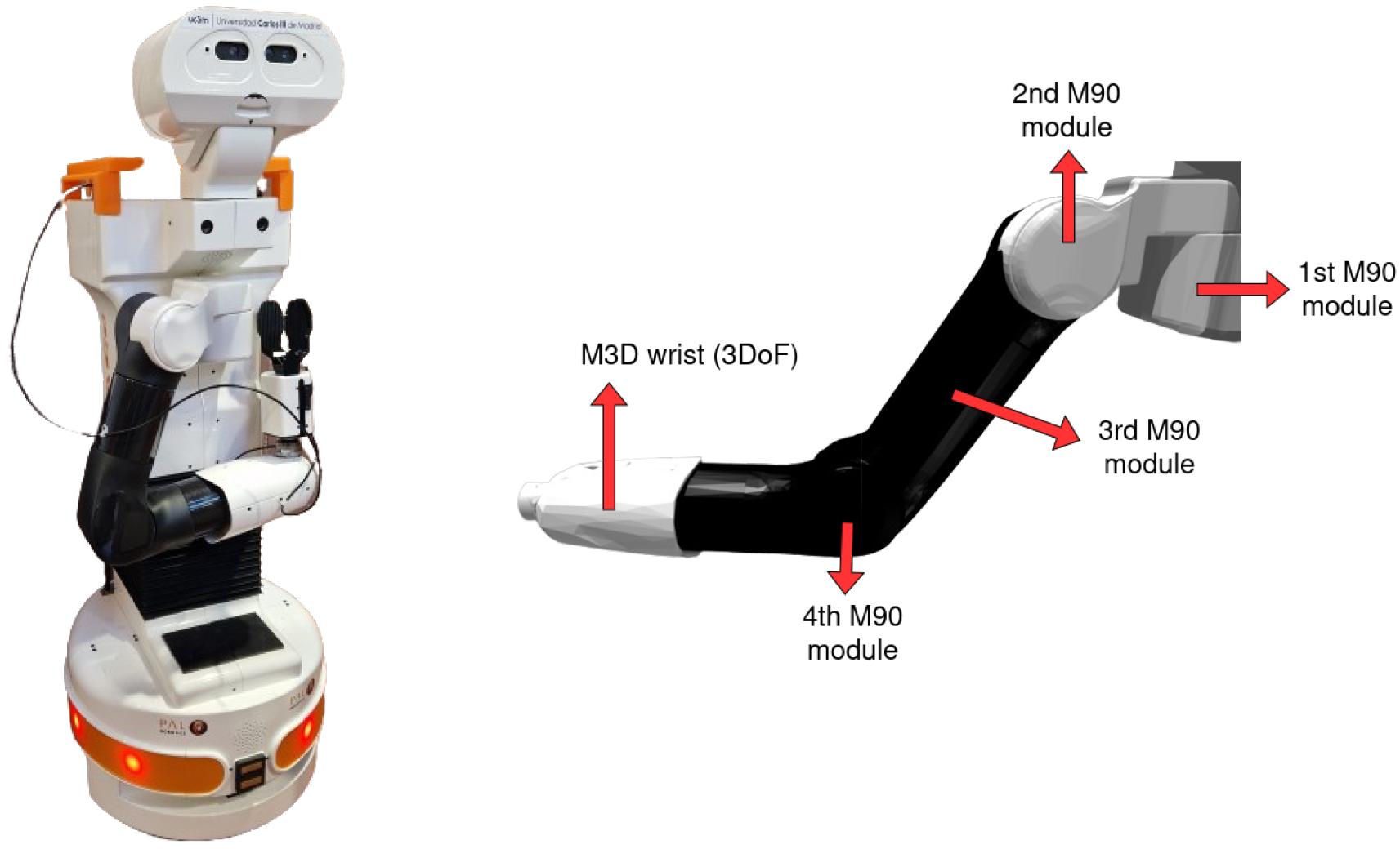
24], and features 7 degrees of freedom (DOFs). The first four DOFs are part of the arm and are powered by brushless motors, while the remaining three DOFs are part of the wrist. A force-torque sensor can be attached to the end effector of the wrist, enabling the arm to be compliant by detecting excess force during grasping and halting motion if needed. TIAGo can be configured with one arm or two arms (TIAGo++). Without the end effector, the arm has a lifting capacity of up to 3 kg. An image of TIAGo and the structure of its arm can be seen in
Figure 1.
It is relevant to note that even though TIAGo is a mobile robot, it is not treated as such in this study. Every joint except for those in the manipulator arm has been blocked, which means that, through every stage of the training, the robot is in a fixed position and can only move the 7 DOFs corresponding to its arm. By doing this, the IK solver system has been made independent from the rest of the robot, following the modular design of TIAGo. In a real-world application, the base or any other joint could be controlled by a different system providing an advantage over stationary robots. However, this is outside the scope of the study and is left as future work.
2.2. Dataset Generation
To apply a supervised learning approach to the challenge at hand, the first step consists of the creation of a labeled dataset. Two different generation methods are proposed and implemented for this purpose: random pose generation with motor babbling in a simulated environment and random pose generation with Forward Kinematics (FK). The output of both methods will be a CSV file containing joint space positions and the corresponding Cartesian space poses of the robot arm end-effector. No data on trajectories or joint velocities were collected, as this is not in the scope of this project, which solely focuses on the static IK transformation.
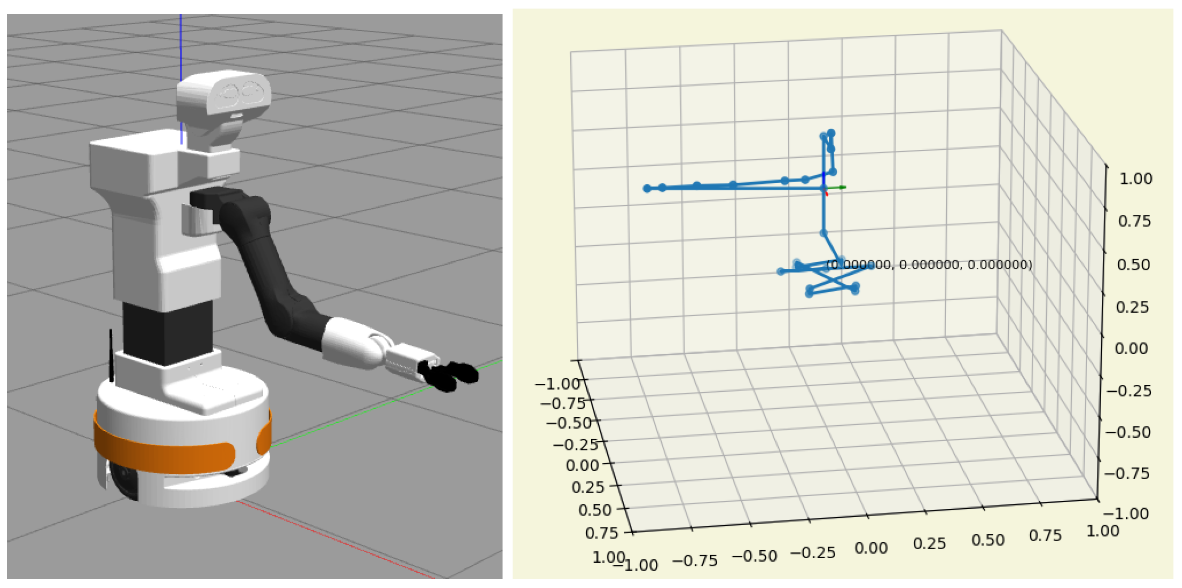
Motor babbling is the process of repeatedly performing random joint space commands for a short duration. In this particular case, the action is performed in a simulated environment using the Gazebo robot simulator [
26] as seen in
Figure 3, which emulates the environment’s physics and implements the robot’s low-level software components known as ROS controllers. The first generation method is based on creating an ROS controller that generates random joint space goals and records the robotic arm’s end-effector poses as it moves towards them. The joint space positions and end-effector poses thus generated are more realistic than those generated by other means, as they do not depend on the ideal implementation of Forward Kinematics but on the readings of the simulated poses themselves.
The software ROS controller is implemented using the
ros_control framework [
27]. TIAGo’s default arm ROS controller is stopped and a custom one is loaded in its place. This one writes the CSV header upon starting depending on the orientation representation, and generates a pose by sampling random joint space positions between each of their upper and lower limits. A command is then generated and followed until a joint is close to its destination, in which case a new goal is generated for it. The end-effector position is read from the simulator at each point, with readings too close to the floor being discarded and not included in the dataset. When the desired number of points is reached, the ROS controller is stopped and the default arm ROS controller is loaded again.
The second generation method makes use of an FK module to transform random joint space positions into end-effector poses. This method is less reliable as it depends on an ideal FK module which may not give as realistic a result as provided directly from the simulator readings. On the other hand, it is considerably faster and less resource consuming.
The implementation of this second method is based on
pykin, a python-based robot kinematics library built upon
ikpy (see
https://github.com/Phylliade/ikpy, accessed on 8 May 2025) and
kinpy (see
https://github.com/neka-nat/kinpy, accessed on 8 May 2025). The script loads a model of TIAGo from URDF and writes the header of the CSV file depending on the chosen orientation. Then, it generates random joint space positions between their upper and lower limits, computes the Forward Kinematics and saves the position and orientation of the end-effector. Points are discarded if they are too close to the floor or too far from the first joint (the shoulder). A representation of this method, the
pykin visualizer, can also be seen in
Figure 3.
Independently of the chosen generation method, the final result is a CSV file containing the desired number of rows with the positions of the arm_1 to arm_7 joints and the resulting end-effector position and orientation if desired. As was mentioned before, the first method is more realistic; however, it can take up to an hour to generate a test dataset of 10,000 samples due to it needing to simulate the movements. The second method, on the other hand, takes less than a minute. For this reason, and because the FK module is needed to calculate position and orientation errors during validation, the second option is preferred in this case.
2.3. Dataset Preprocessing
Once generated, the dataset needs to be preprocessed before it can be fed to a neural network for training. The data are read and transformed into a pandas data frame, from which some statistical markers are computed. For each column, the minimum, maximum, absolute maximum, mean, median, standard deviation, first quartile, and third quartile are computed and saved to a YAML file, to be used in case the operations performed during preprocessing need to be reversed. Since there are many possible solutions to the IK problem, it is possible that samples have been generated with the same pose as the input but different joint space positions as the output. Therefore, before processing the data any further, input duplicates are removed to ensure the network trains on unique input–output pairs.
Dataset scaling, or normalization, is a crucial preprocessing step in a machine learning pipeline. Its purpose is to adjust the scale of values so they all fall within the same range. This transformation is known to enhance the performance of neural network models, and there are various scaling techniques available from which to choose [
28]. In this study, four options are proposed, given by the following formulas:
Min–max normalization (Equation (
1)) rescales the data such that all values are in the
range. Standardization (Equation (
2)) removes the mean and scales the data to unit standard deviation. They are both very sensible to the presence of outliers. Max–absolute scaling (Equation (
3)) is similar to min–max normalization, behaving in the same way when all values are positive. When the dataset contains positive and negative values, which is the specific case of this dataset, the data are scaled to the
range. It is affected by large outliers as well. Robust scaling (Equation (
4)) is based on quartiles, as it makes use of the interquartile range (IQR), which is defined as the difference between the third and first quartiles. It is not as influenced by outliers as the other options. The resulting range is, additionally, larger than for the other scalers.
After the normalization step, the data are split into training, validation, and test sets following a 70–20–10 rule. All three sets are generated in the same step, following the strategy described in
Section 2.2, and then split and saved into separate
numpy files (
.npy) for their corresponding use.
Finally, the training set can be split into a number of curriculums. If only one curriculum is requested, the neural network will be trained with all available data from the beginning. In any other case, it will start by training on the points closest to the robot, which are easier to learn, and move to further points as it progresses. The division can be performed by quantiles so that each curriculum holds the same number of points, or by distance so that when moving to a new curriculum, the distance to the furthest point will always increment by the same number. Each curriculum contains the previous one so the neural network already knows some of the data.
2.4. Deep Neural Network Models
Once the data are generated and preprocessed, the next step is to build the DNN models that will be used to train on these data. This section explores the different DNN models used in this study to address the Inverse Kinematics problem. When training, the inputs and outputs are inverted with respect to the dataset generation step. For every DNN model described, the input vector specifies the desired Cartesian target for the end-effector, , and the output vector comprises the corresponding joint space positions that obtain this target, .
Three Multilayer Perceptrons, two Recurrent Neural Networks, and a Convolutional Neural Network have been built and tested. In the following subsections, the architecture of each model is examined, highlighting their strengths and potential use cases in solving IK tasks, and specifying the best hyperparameters found for each model through testing. The models have been built using Keras and have an associated YAML file where the hyperparameters can be easily set and changed.
2.4.1. Feed-Forward Multilayer Perceptron
The Feed-Forward Multilayer Perceptron (MLP) is a widely used Deep Neural Network (DNN). In the context of Inverse Kinematics (IK), it serves as a model that represents a non-linear relationship between the input vector (specifically, the desired Cartesian target for the end-effector,
) and the output vector (the corresponding joint space positions that obtain this target,
). Each MLP consists of an input layer, multiple hidden layers, and an output layer [
29].
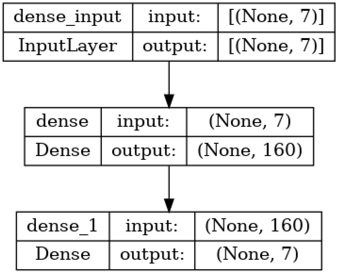
Three different MLPs are built to solve the IK problem. The first of them consists of an input layer, one hidden layer, and an output layer. The input and output sizes are set depending on the shape of the training dataset. The number of neurons in the hidden layer has been optimized using a hyperparameter tuner, and finally set to 160. An instance of this architecture can be seen in
Figure 4. The hidden layer makes use of the
ReLU activation function while the output one, after multiple tests, uses the
tanh activation function. This first MLP will be referred to as SimpleMlp.
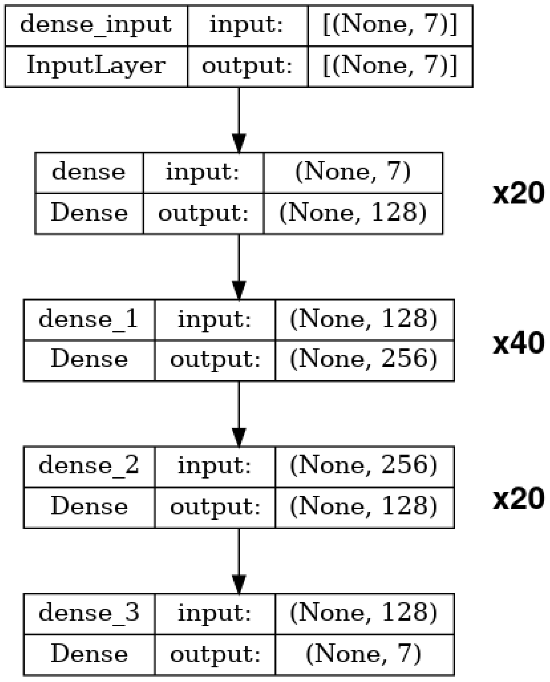
The second proposed MLP architecture expands on the first one, adding more hidden layers. Specifically, the model consists of an input layer, 80 hidden layers, and an output layer. The first and last 20 hidden layers contain 128 neurons each, while the middle 40 hidden layers contain 256 neurons each. The input and output sizes are again set depending on the shape of the training dataset. An instance of this architecture can be seen in
Figure 5. As before, the hidden layers use
ReLU as their activation function, and the output layer uses the
tanh activation function. This second MLP will be referred to as DeepMlp.
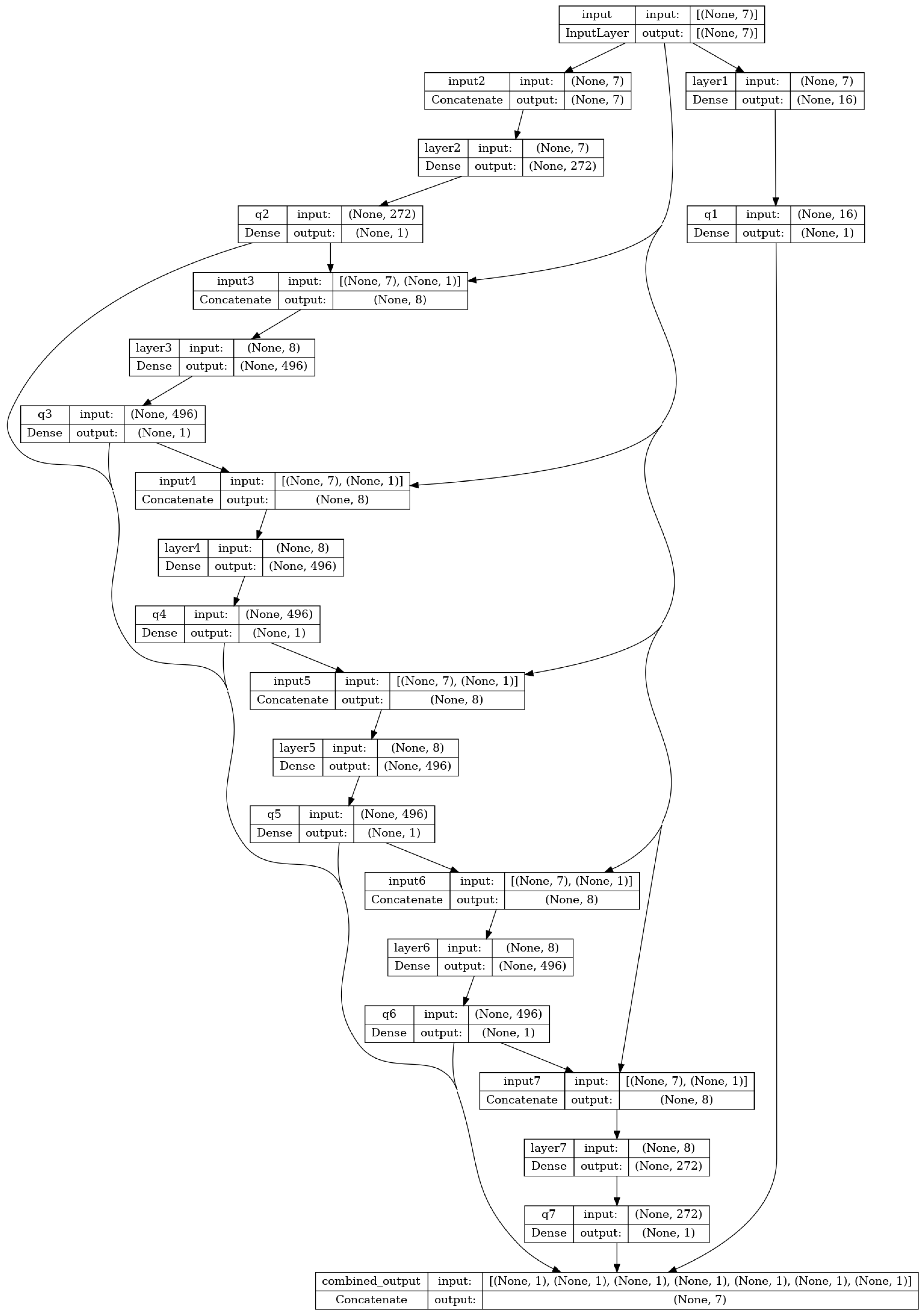
Finally, the third model follows the idea of [
30], where each joint has an associated subnet with one hidden layer. The original architecture is expanded to include TIAGo’s 7 DOFs and therefore contains one input layer, 7 subnets, and one output layer, as can be seen in
Figure 6. The units for each subnet are set to 16, 272, 496, 496, 496, 496, and 272, respectively. All layers use a
linear activation function. It will be referred to as SubnetMlp.
2.4.2. Convolutional Neural Network
Convolutional Neural Networks (CNNs) are typically made up of convolutional and pooling layers. In addition, fully connected layers (also referred to as dense layers) are often included near the network’s output. The convolutional layers consist of input data, a filter, and a feature map, enabling the CNN to identify key features in the input data. Pooling layers perform downsampling, which helps reduce the number of parameters in the input. Lastly, fully connected layers ensure that each node in the following layer is directly linked to a node in the previous one. While CNNs are mainly used for tasks related to image processing and recognition, they can additionally be applied to other areas, including solving Inverse Kinematics (IK) problems.
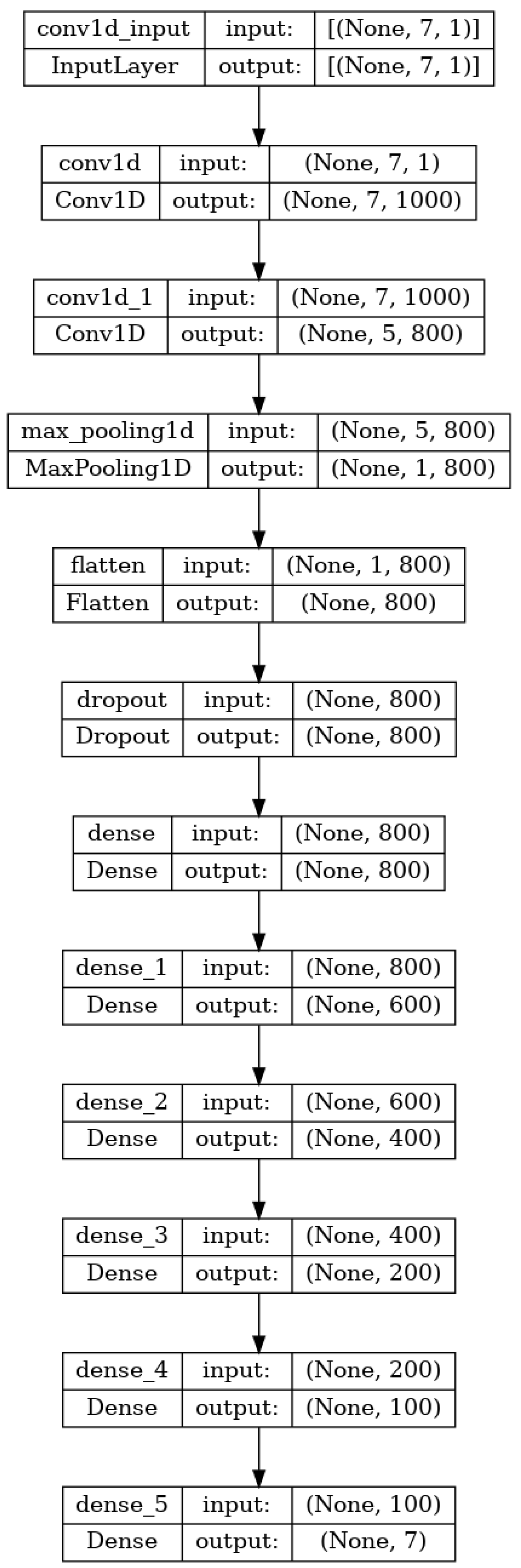
The proposed CNN follows the idea of [
12]. The network contains 8 hidden layers, the first 2 being convolutions. After that, if the input size is big enough, a pooling layer can be added before a dropout and 5 fully connected layers. An instance of this architecture can be seen in
Figure 7. In the case of the input containing only position and not orientation, the pooling layer has to be removed as not enough parameters are provided. The layers use
ELU as their activation function. It will be referred to as CNN.
2.4.3. Recurrent Neural Networks
Recurrent Neural Networks (RNNs) are deep learning models designed to handle sequential data, making them ideal for working with time-series data. In this context, inputs and outputs are interdependent and can influence the processing of subsequent data. RNNs include a recurrent unit that functions as a memory mechanism, enabling the network to learn from previous inputs. There are three primary types of RNN units available: Gated Recurrent Units (GRUs), Long Short-Term Memory (LSTM), and Bilateral Long Short-Term Memory (BiLSTM).
Two different RNNs have been built to solve the IK problem. Similar to the MLP case, the first of them consists simply of an input layer, one hidden layer, and an output layer. In this case, however, the hidden layer is not a fully connected (dense) layer but a recurrent layer. It consists of 12 fully connected neurons, where the output is to be fed back as the new input. An instance of this architecture can be seen in
Figure 8. The output layer uses the
tanh activation function. It will be referred to as SimpleRnn.
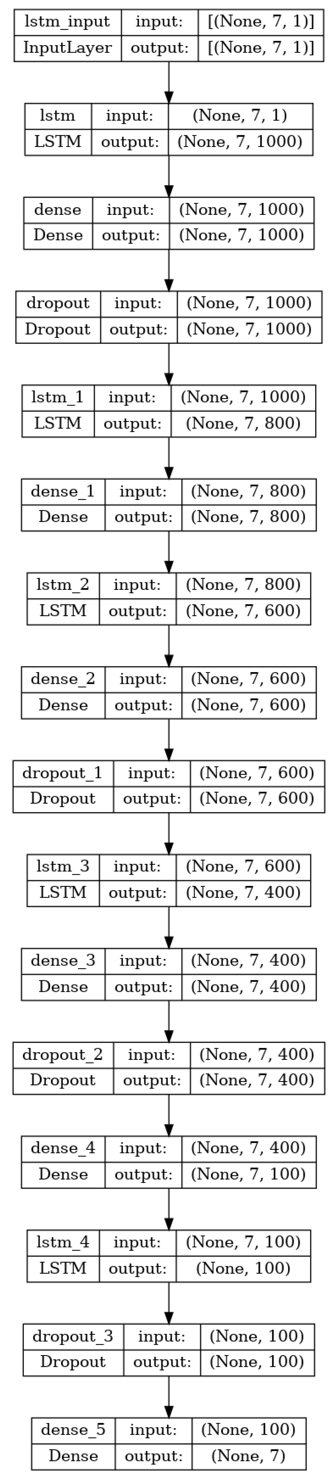
The second proposed RNN is an LSTM network, built after the one presented in [
12]. It consists of 5 LSTM layers and 6 fully connected hidden layers. To decrease the issue of over-fitting, a dropout of 0.2 rate is added after each fully connected layer. An instance of this architecture can be seen in
Figure 9. The hidden layers use
swish as their activation function and the output layer uses the
linear activation function. It will be referred to as LSTM.
2.5. Training Loop
Once the previous steps are finished, the training loop is designed. The script which runs this loop, written in Python 3.11, takes the name of a DNN model as an input parameter. Based on the name, an instance of this model is created, and its associated YAML configuration file, which contains the model hyperparameters, is loaded. This file additionally contains the path to the desired preprocessed dataset, and therefore its associated statistics file. The statistics file, as mentioned before, contains the number of curriculums generated, the number of samples in each curriculum, the normalization technique used, the percentage of samples used for testing, and the statistical markers for each column of the dataset. The path can be manually set by changing the configuration YAML.
For the training and validation data, generator functions are used. These receive the batch size and are informed of the current curriculum via a global variable. They load the corresponding data from .npy files and choose random elements from them until they fill the batch which is then returned.
The models are compiled using mean squared error as the loss function and Adam as the optimizer. Metrics include mean squared error, position error, and orientation error. These last two metrics follow a custom implementation and require activating run_eagerly on the training to allow access to the ground truth and predicted values for each epoch. The custom metrics can be added to the training as metrics or as callbacks. The results are more precise in the first case as they are incorporated within each iteration of the internal loop, however, they are more time and resource consuming.
The learning rate (LR) for every model is initially set to 0.1 and decreases progressively according to a modified version of the Keras callback ReduceLROnPlateau. This callback monitors one of the metrics and if no improvement is seen for a provided number of epochs, the learning rate is reduced by a factor. In this case, the callback has been modified to update the curriculum number if no improvement is found for the validation loss metric and the LR is at its minimum. When the curriculum number is changed, the LR goes back to its original value and starts decreasing again after a cooldown number of epochs. If the total number of curriculums is reached, the training stops. The pseudocode for this method can be seen in Algorithm 1.
The number of training iterations is set to 500 as a maximum. However, the training will stop following the logic of Algorithm 1 when no improvement is detected and the LR is at its minimum.
| Algorithm 1 method on_epoch_end for callback class UpdateLRCurriculumOnPlateau |
ifthen end if ifthen else if then if then if then else if then else if then stop training end if end if end if end if end if end if
|
3. Experiments and Results
In this section, the results obtained during and after training the proposed models are discussed. First, the metrics used to study the precision of each model are explained, focusing on the formulation of the position and orientation error. After this, all the experiments are detailed, dividing the results by normalization technique, orientation representation, and architecture. Finally, the effects of curriculum learning are studied.
For each experiment, the provided plots represent the results obtained for each metric on the validation data. This data is not used during training or seen by the model; however, it is used to tune the hyperparameters. Therefore, a table is additionally provided for each experiment that shows the performance of the model on a completely separated and previously unseen set of test data.
3.1. Metrics
To study the performance of each proposed model in solving the IK problem, different metrics have been used. As was mentioned before, the mean squared error has been used as a predefined metric. Additionally, the position and orientation error have been implemented as callbacks and added to the training.
For the position error, the three-dimensional Euclidean distance has been employed. However, for the orientation error, a range of options have been considered after studying the options brought forward by [
31,
32,
33]. To select a metric, the orientation representation has to be taken into account, as it depends on whether quaternion or rotation matrices are being used. Euler angle representations have not been considered since they are not as accurate [
34].
In case the orientation is defined using unit quaternions, three possible errors are defined:
As [
31] notes, Equation (
5) defines a
pseudometric since
but
. However, the mapping from unit quaternions to SO(3) is 2-to-1, meaning that there are two possible unit quaternions for every rotation angle (
q and
). Therefore, the proposed
pseudometric becomes a metric on 3D rotations. It gives results in the range
. The option given by Equation (
6) measures the angle between the two unit quaternions, restricting the angles to the first quadrant. The use of the vector dot product · with unit quaternions means that
. This metric gives results in the range
. Finally, Equation (
7) gives an estimate of the length of the geodesic path on the 4D unit sphere between the two quaternions. Its results are in the range
.
If, instead, the orientation is defined using rotation matrices, four possible errors are considered:
The first metric, given by Equation (
8), measures the angle of the difference rotation matrix between
and
, which is given by
. The second option, stated in Equation (
9), represents the Euclidean metric for rotation matrices, given by the Frobenius norm of the difference between two rotation matrices. Another possible choice is the one given by Equation (
10), which represents the Riemannian distance between two rotations. It is the length of the shortest geodesic curve that connects
and
. Finally, Equation (
11) comes from a general
metric defined in [
35], and is in the range
.
3.2. Experiments
After generating the data and preparing the models, a number of experiments have been conducted varying the parameters of the models as well as the data. The data are generated for the arm of TIAGo, the robotic mobile manipulator described in
Section 2.1, and the inputs and outputs of the models are set accordingly. All the experiments were run using an NVIDIA GeForce RTX 2050. The metrics have been logged during training and validation using Weights and Biases with Tensorboard, and the most relevant results are presented.
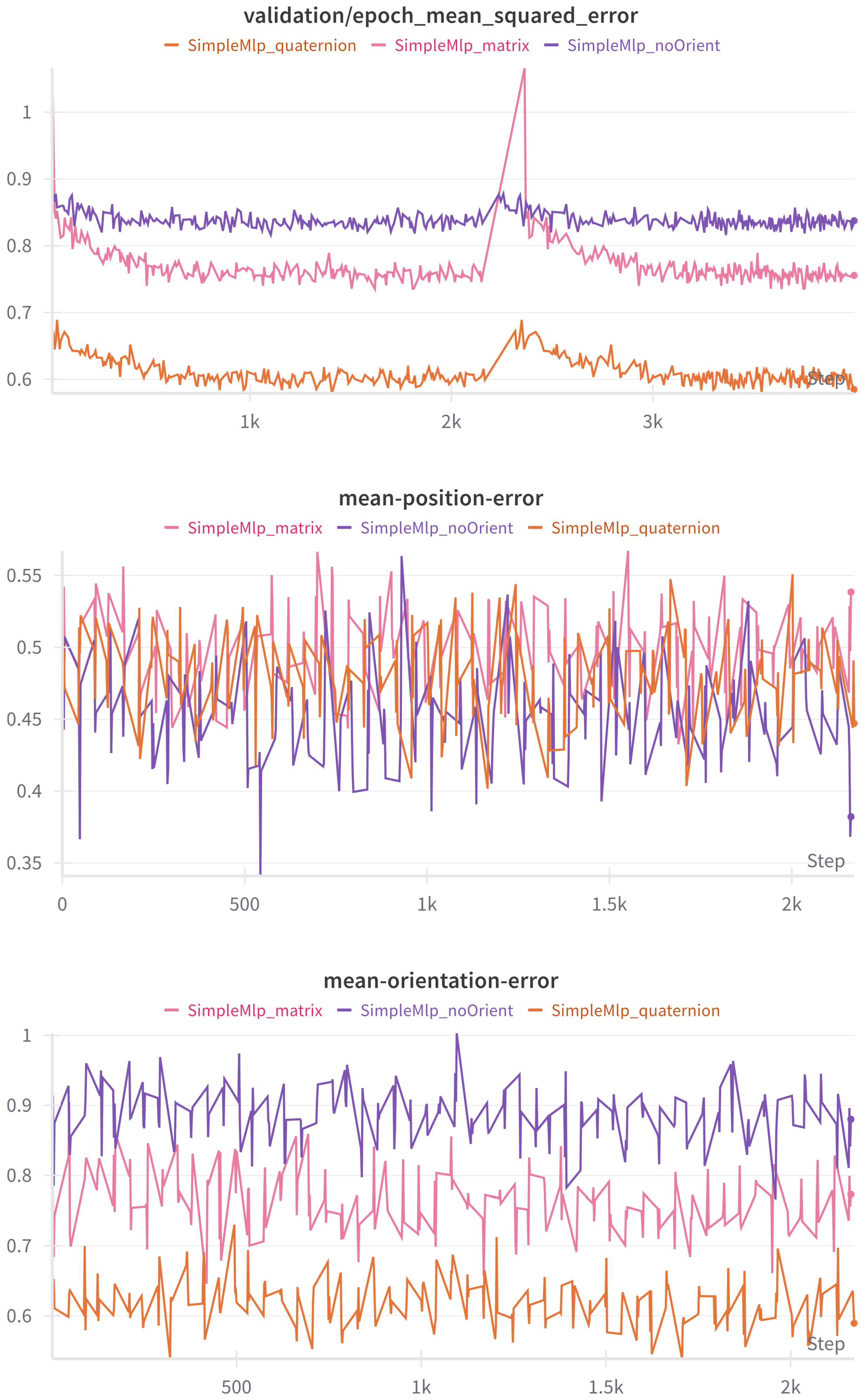
3.2.1. Orientation
First of all, the orientation representation is studied. For this, two custom callbacks are created that compute the position and orientation error. The position error callback takes a batch of validation data, predicts the output from the given input, de-normalizes the ground truth and predicted values, and solves the Forward Kinematics (FK) for the predicted output. With the ground truth and predicted positions, the mean error is stored as the batch mean of the Euclidean distance between the ground truth and predicted values. The orientation error callback proceeds in the same way but solves the FK for both the predicted and ground truth outputs, obtaining the quaternion orientation for both, independently of the input. The error is then computed following Equation (
5).
The results can be seen in
Table 2 and
Figure 10. As expected, when the orientation is not considered, the MSE loss rises. The quaternion representation performs significantly better than its counterparts in every aspect except the position error, where they are all on par. The option with no orientation achieves slightly better results for position. This one, as anticipated, performs worse on the orientation error. The difference in position error is not significant between quaternion and rotation matrix representations; however, the gap in loss and orientation error is noticeable. This is ascribed to the DNNs performing better with fewer input parameters (7 for quaternions, 12 for rotation matrices).
In light of all the above, the quaternion representation is preferred from this moment on. The sudden spikes that can be seen in the first plot are due to no normalization being applied to the dataset, which will be fixed in the next subsection.
3.2.2. Normalization Types
Once the orientation representation has been set, the question of which normalization technique to use, if any, is tackled. Each model was trained and validated with the five possibilities described in
Section 2.3, and the results were mostly similar for all models. For illustration purposes, only the validation results of the SimpleMlp model are presented.
As can be seen in
Table 3 and
Figure 11, the best results are obtained when using max–absolute normalization or robust scaling normalization. The MSE loss fares better for the former; however, the position and orientation error seem to favor the latter. It is, nevertheless, relevant to note that the position and orientation error are not influenced by the normalization in that they are calculated over de-normalized inputs and outputs. The MSE loss, on the other hand, is computed over a normalized dataset. Therefore, as the robust scaling technique yields the lowest position and orientation error, it is preferred over the other options.
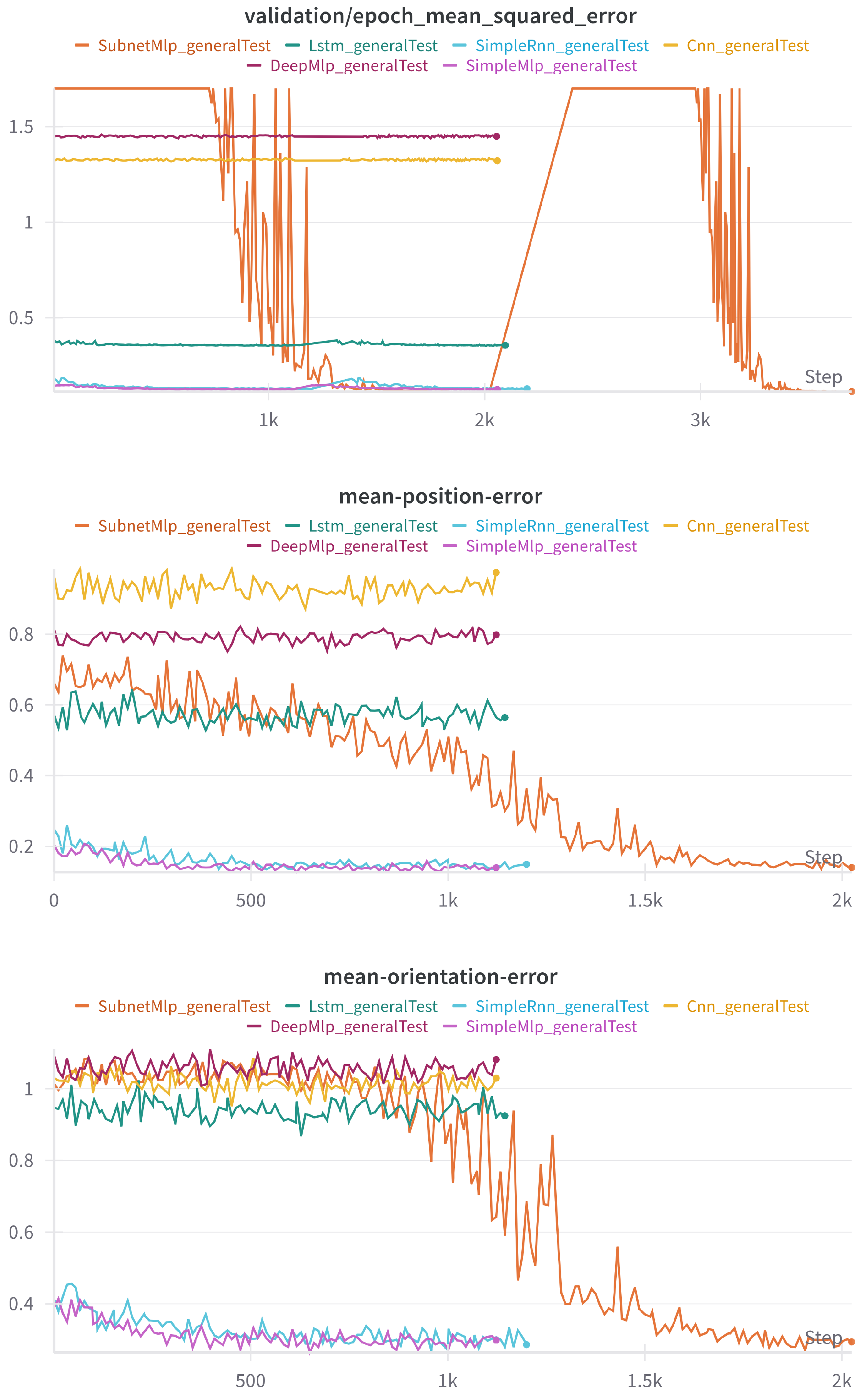
3.2.3. Deep Neural Network Models
To compare the performance of all the proposed models, a dataset is generated with 100,000 samples using quaternions to represent orientation. The dataset is preprocessed and normalized using robust scaling, then fed to all the models for comparison. In every case, the learning rate is reduced using the callback described in Algorithm 1, starting at 0.1 and ending at 0.0001. Only one curriculum is generated. The total data generation time is 1 min and 40 s.
Table 4 collects the results for each metric after training, testing the models on a previously unseen set of data. In
Figure 12, the MSE loss, position error, and orientation error for every model can be seen. For the position error, the Euclidean distance is used, the units being meters. For the quaternion error, the chosen metric is the pseudometric given by Equation (
5), meaning the results are in radians and, in particular, in the
range. All three plots represent metrics evaluated on the dataset apart from validation at the end of each epoch. Rather than attempting to provide statistical relevance, the results intend to be descriptive.
The variance of the output columns in the dataset is 1.2284, which means that most models have an acceptable MSE according to the R2 metric, where R2 is defined as , except for the CNN and DeepMlp models. This, in opposition to the performance of the SimpleMlp and SimpleRnn models, both with only one hidden layer, points to the conclusion that increasing the depth of the DNNs used does not necessarily lead to better performance when dealing with the IK problem.
It can be seen, both in the plot and in the results, that the best-performing model is the SubnetMlp one (
Figure 6). It is additionally the most affected by the learning rate decreasing callback (Algorithm 1), since every other model, although decreasing slightly with the change in learning rate, mostly seems to stabilize quickly, while the descent in this case is steeper.
The performance of both RNNs and the SubnetMlp highlight the importance of considering the dependencies between joints when dealing with the IK problem. In the RNN case, this is implicit in its memory as it takes into account past results while it is learning. In the SubnetMlp, it is explicit in the model architecture, as each subnet takes the results from the previous one as an input.
Regarding training time, it is to be noted that simpler architectures such as SimpleMlp and SimpleRnn took three times less time to train than the more complex models.
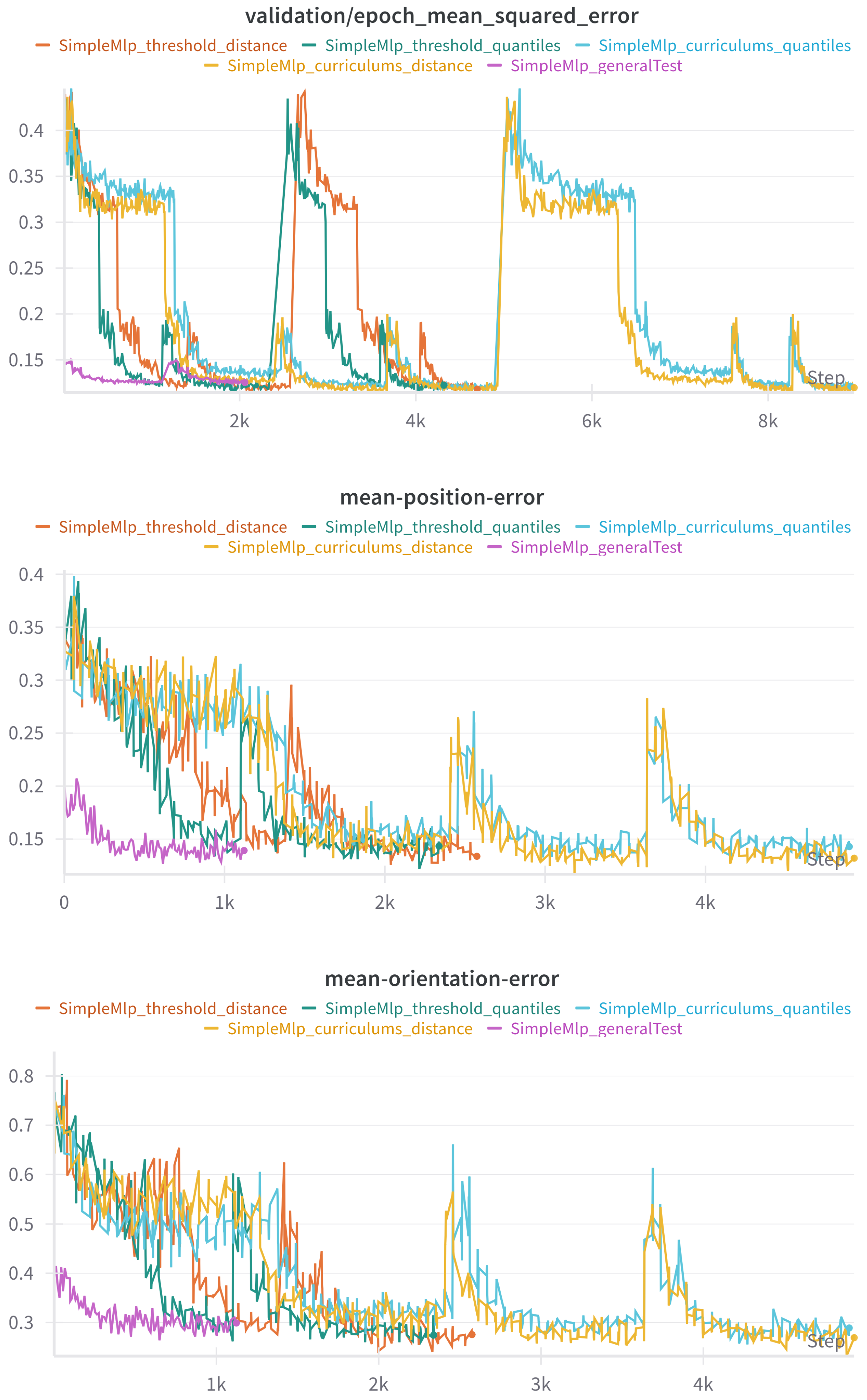
3.2.4. Curriculum Learning
The next step will be to study the effect of curriculums on the training. To perform this, a new dataset is generated, containing 100,000 normalized samples, using quaternions for the orientation. The dataset is then divided into four curriculums, following two different approaches. In the first, the boundaries for each curriculum are distributed so that each slice encompasses the same distance. In the second, the boundaries are chosen so that each slice contains the same number of samples. Each curriculum is then built containing the previous ones.
With the idea of reducing training time and of preventing overfitting, a new version of the UpdateLRCurriculumOnPlateau callback (Algorithm 1) is written. In this case, the change of curriculum occurs when a certain threshold is reached for the validation loss. The threshold starts at 0.3 and decreases every time a new curriculum is loaded.
All possibilities are tested with the SimpleMlp model, and the results can be seen in
Table 5 and
Figure 13. As before, the plots contain measures taken with the validation data during training, and the table contains the metrics tested on a separate dataset.
The best results are obtained when the model is training with curriculums distributed by equal distance, using the version of the callback described in Algorithm 1, where the curriculum is changed once the learning rate is at its minimum. However, the difference between metrics for the difference options is minimal.
This leads to the threefold conclusion that, within the scope of the tests conducted, the changes applied to the training scheme are not relevant to the results. In the first place, the use of curriculums, as opposed to training with only one dataset, makes only a minor impact, barely improving the metrics. Secondly, the choice of boundaries for the curriculum generation is irrelevant. Finally, using a threshold to decide when to change curriculums does not reduce training time or enhance the performance of the models.
To sum up, although curriculum training has been shown to improve other training schemes for IK, such as DRL control, the specific strategies tested here do not seem to affect supervised learning. It remains possible that alternative curriculum designs could yield different outcomes.
3.2.5. Comparison with Classic Methods
To ascertain the practical value of the DNN approach to the IK problem, the results have been compared to those obtained by means of more traditional methods. In this experiment in particular, the best-performing DNN model will be compared against the Orocos KDL IK solvers (See
https://www.orocos.org/wiki/Kinematic_and_Dynamic_Solvers.html, accessed 24 May 2025). To do this, the kinematic chain of the robotic arm is created and the test dataset used to evaluate the DNN models is loaded. The values are de-normalized, and, for each Cartesian pose input, the IK is computed using a classic solver. The resulting joint space positions are compared to the expected ones and the mean squared error is obtained.
The tested options include two position IK solvers based on a numerical approach. The first of them is based on the Newton–Raphson method, an iterative algorithm which produces an approximation to the root of a function by refining an initial guess. The second solver is based on the Levenberg–Marquardt algorithm, used to solve non-linear least squares problems. The initial guess for both solvers places every joint at 0 radians, which approximately sets each one of them halfway through its upper and lower limits. It is the default starting point for many manipulation tasks that employ the TIAGo robot. No sensitivity analysis has been performed.
The results of the comparison can be seen in
Table 6. They include the mean squared error, the number of times a solution could not be found for a given input, and the time needed to process the whole test dataset.
As can be seen, the results suggest that the DNN approach may offer some advantages over the proposed Jacobian-based numerical methods. While the mean squared error favors the DNN method, it might be influenced by the choice of initial guess in the numerical algorithms and should therefore not be deemed as relevant a result. Notably, the numerical methods fail to converge in approximately 13% of the test cases, whereas the DNN consistently provides a solution. Additionally, it takes considerably less computation time. Overall, this experiment indicates that the DNN approach holds promise as an alternative for solving the IK problem. However, further investigation is needed.
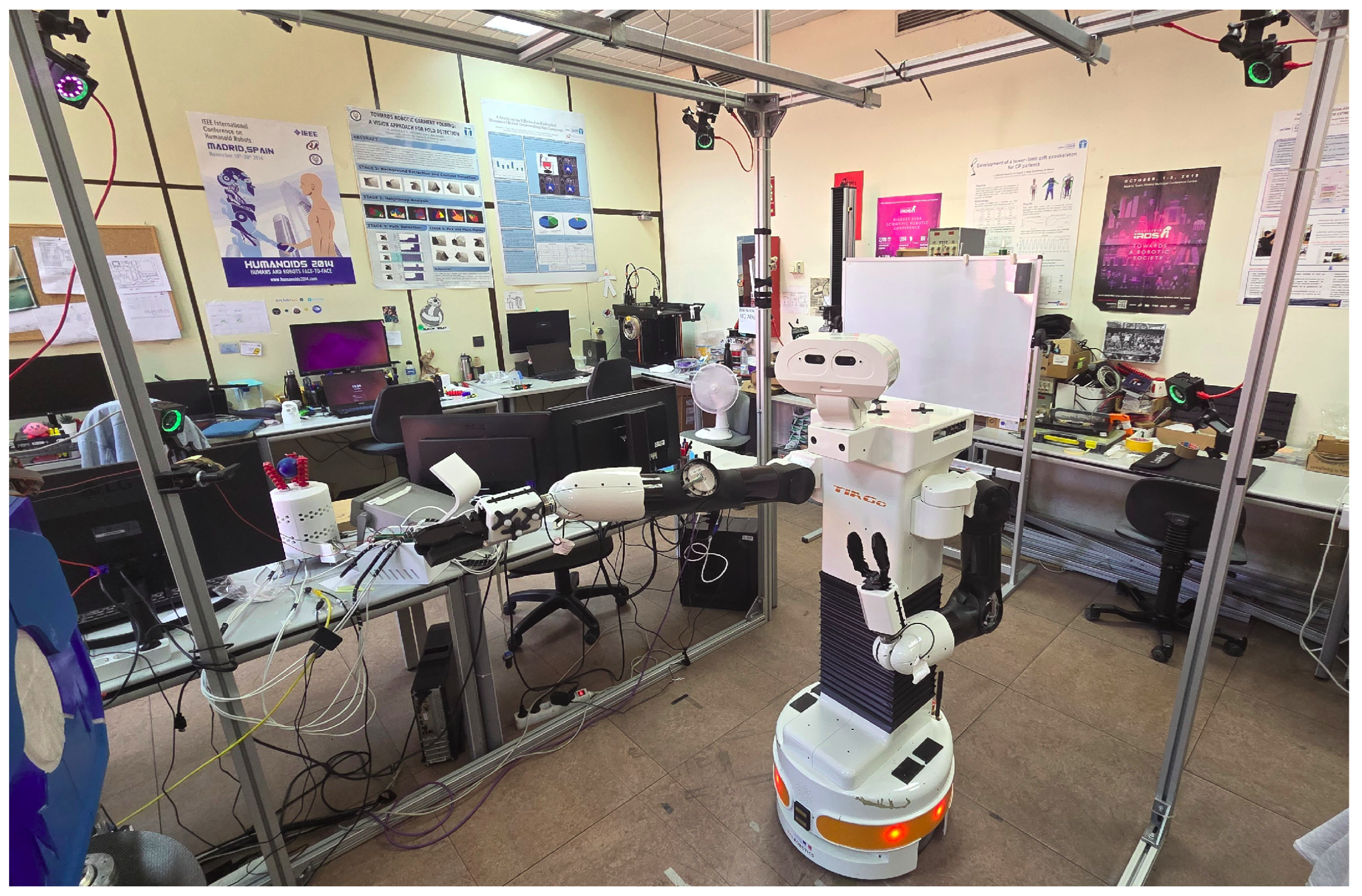
3.2.6. Sim2real Transfer
To test the performance of the presented DNN-based IK solver on the real robot, the following experiment is performed. The robot is placed inside a motion capture structure as can be seen in
Figure 14, with markers placed on its end-effector.
As a technicality, while in simulation, the ROS controller could be bypassed and joint space positions resulting from the inference could be directly commanded to the robot. The real robot requires the actual robot ROS controller, as commanding the resulting joint space positions directly without a low-level controller might result in a crash. Therefore, the inference here is implemented as an ROS package which is a layer of abstraction above the robot ROS controller. It is designed as a software component to allow the user to specify a Cartesian space target and enable the robot’s low-level software controllers to receive a joint space target. As such, once it receives a goal in the shape of a Cartesian 3D position and quaternion orientation, it is normalized and fed to the DNN model, which has been previously loaded. The resulting output is de-normalized and sent to the low-level controller of the robot’s arm. This way, it is the robot’s own planner and controller which execute the movement, and the DNN is exclusively used for IK purposes. Therefore, we can obviate dynamic effects internal to the ROS controller and focus only on the study of the IK transformation, which is static.
The IK solvers transform the Cartesian space target into the joint space target. When transitioning to the real robot, two additional errors are introduced. The first error is at the joint level, which is the discrepancy between the joint space target and the joint space position actually achieved (as read by the encoders).
Table 7 describes this error, both in terms of joint space error, as well as the transformation of each of these two components via Forward Kinematics to depict the magnitude of this error in the Cartesian space.
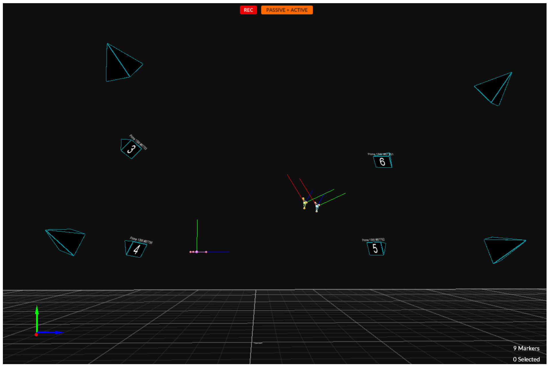
The second error is due to all other mechanical aspects, such as additional tolerances and small mechanical deformations of the links. This kind of error may only be measured by external devices that serve as a ground truth. As presented in the beginning of this section, a motion capture system has been introduced to quantify this source of errors, which is a common design decision when opting for a ground truth. Motion capture markers have been placed on the robot’s tray surface to mark its position with respect to the world coordinate system. To detect the end-effector position, six markers have been placed on the flat surfaces on both sides of the gripper. An illustration of the points detected by the system can be seen in
Figure 15.
Table 8 describes this error, comparing the expected Cartesian space position given the joint space position actually achieved (as read by the encoders) and transformed to this space via Forward Kinematics, versus the motion capture system detected positions, to depict the magnitude of this error in the Cartesian space with respect to the corresponding ground truth.
Finally,
Table 9 includes the summary of results, providing the mean and standard deviation corresponding to both errors. Error 1 refers, as explained, to the distance between the points ideally reached by the desired joint space configuration and the one given by the encoder readings. Error 2 refers to the difference between the ground truth given by the motion capture system and the FK computations performed on the real joint positions achieved by the robot. Finally, the global error corresponding to the difference between the FK transformation of the joint space targets and the motion capture readings is displayed. In position, the global error is more affected by Error 2, which is larger than Error 1, which is visible by orders of magnitude. Errors in position derived for each type of error are similar.
4. Conclusions
In this paper, we have introduced an approach for solving the Inverse Kinematics of the robotic arm of TIAGo using methods based on supervised Deep Learning algorithms (MLP, CNN, and RNN) and putting the focus on static transformations, setting aside joint velocities or trajectories. The complete pipeline has been presented, including data generation and preprocessing, training, and validation. The effect of orientation representation and data normalization has been studied, and different DNN models have been built and evaluated. Finally, the effect of curriculum learning on the training scheme has been studied.
The evaluation of different orientation representations highlights the impact of incorporating orientation as an input to the IK problem to achieve higher precision. Among the methods tested, the quaternion-based definition proved to be the most effective. This approach stands out because it creates fewer input parameters than rotation matrices, while still delivering robust results. These findings suggest that quaternions are a promising and efficient option to represent orientation in DNN-based IK applications.
Based on the findings of this study, it is evident that data normalization appears to play a crucial role in improving the performance of DNNs applied to the IK problem. Various normalization techniques were tested, and the results suggest that preprocessing can be an essential step in the training pipeline. Among the techniques evaluated, robust scaling yielded the best results, performing similarly to max–absolute normalization. This suggests that robust scaling is an effective choice for IK data preprocessing, as datasets representing poses in Cartesian space and joint space positions are prone to contain outliers or varying feature scales.
The testing of various models indicates that even small and simple architectures can achieve position and orientation errors comparable to those of larger models after sufficient training. Notably, Recurrent Neural Networks (RNNs) were among the best-performing models, as they are capable of capturing the temporal dependencies and relationships between joint movements. This ability to consider the sequential nature of joint interactions likely contributes to their superior performance in the IK problem. However, the best performing model consisted of a feed-forward neural network which explicitly takes into account the dependencies between joints by using a subnet to represent each one. The outputs of the preceding subnet are fed as an input for each of these along with the target position and orientation. These findings hint at the importance of joint dependencies for the IK problem. Further research may explore additional enhancements to DNN models, such as incorporating attention mechanisms or hybrid approaches, to further boost their performance.
While curriculum-based training has shown benefits in other contexts, its impact on solving IK problems within the scope of this project using DNNs appears to be minimal. Our experiments show that, in this case, training with evenly distributed curriculums, along with the callback method for curriculum adjustment, yields only slight improvements in performance. Specifically, the choice of curriculum boundaries and the threshold for transitioning between curriculums do not significantly affect the model’s training time or accuracy. Thus, the suggested curriculum training strategies do not provide a substantial advantage in supervised learning for IK problems. Further investigation is needed into alternative curriculum designs, which could yield different outcomes.
The practical value of the DNN approach to the IK problem has been assessed by comparing its performance to that of classic numeric solvers. The results indicate that it is both faster and more reliable, and can compete with classic solvers in terms of precision.
Finally, the possible causes of error when transitioning from a simulated environment to a real-world scenario have been studied. The difference between the commanded joint positions and the ones achieved by the robot is minimal; however, even this small displacement causes orientation errors. The second source of errors, ascribed to mechanical aspects of the real robot that cannot be taken into account in a simulated model, adds an additional inaccuracy between the desired target and the reached pose. All of these factors have to be taken into account when trying to deploy one of the methods presented in this study to real-world manipulation scenarios.
Author Contributions
Conceptualization, A.C.-G., J.G.V., F.J.N.-C. and C.B.; methodology, A.C.-G. and J.G.V.; software, A.C.-G.; validation, A.C.-G. and J.G.V.; formal analysis, A.C.-G.; investigation, A.C.-G. and J.G.V.; resources, A.C.-G. and J.G.V.; data curation, A.C.-G. and J.G.V.; writing—original draft preparation, A.C.-G.; writing—review and editing, J.G.V.; visualization, A.C.-G.; supervision, J.G.V., F.J.N.-C. and C.B.; project administration, J.G.V. and C.B.; funding acquisition, J.G.V. and C.B. All authors have read and agreed to the published version of the manuscript.
Funding
The research leading to these results received funding from “iRoboCity2030-CM Cont” (TEC 2024/TEC-62) of Comunidad de Madrid, “iREHAB” (DTS22/00105) of Instituto de Salud Carlos III, and EU structural funds.
Institutional Review Board Statement
Not applicable.
Informed Consent Statement
Not applicable.
Data Availability Statement
The original contributions presented in this study are included in the article. Further inquiries can be directed to the corresponding author(s).
Acknowledgments
In the process of writing, the artificial intelligence tool ChatGPT was employed as a means of enhancing and verifying the accuracy of orthography and grammar of the introductory sections for each chapter and the conclusions. Its outputs were always reviewed and edited by the authors. The contributions and content of the paper are entirely by the authors.
Conflicts of Interest
The authors declare no conflicts of interest.
Abbreviations
The following abbreviations are used in this manuscript:
| DNN | Deep Neural Network |
| IK | Inverse Kinematics |
| FK | Forward Kinematics |
| MLP | Multilayer Perceptron |
| CNN | Convolutional Neural Network |
| RNN | Recurrent Neural Network |
| DOF | Degree of Freedom |
| LSTM | Long Short-Term Memory |
| BiLSTM | Bilateral Long Short-Term Memory |
| GRU | Gated Recurrent Unit |
| LR | Learning Rate |
| IQR | Interquartile Range |
| MSE | Mean Squared Error |
References
- Kucuk, S.; Bingul, Z. Robot Kinematics: Forward and Inverse Kinematics; INTECH Open Access: London, UK, 2006. [Google Scholar]
- Aristidou, A.; Lasenby, J. Inverse Kinematics: A Review of Existing Techniques and Introduction of a New Fast Iterative Solver; University of Cambridge, Department of Engineering: Cambridge, UK, 2009. [Google Scholar]
- Calzada-Garcia, A.; Victores, J.G.; Naranjo-Campos, F.J.; Balaguer, C. A Review on Inverse Kinematics, Control and Planning for Robotic Manipulators With and Without Obstacles via Deep Neural Networks. Algorithms 2025, 18, 23. [Google Scholar] [CrossRef]
- Aristidou, A.; Lasenby, J.; Chrysanthou, Y.; Shamir, A. Inverse kinematics techniques in computer graphics: A survey. In Computer Graphics Forum; Wiley Online Library: Hoboken, NJ, USA, 2018; Volume 37, pp. 35–58. [Google Scholar]
- Semwal, V.B.; Gupta, Y. Performance analysis of data-driven techniques for solving inverse kinematics problems. In Intelligent Systems and Applications. IntelliSys 2021. Lecture Notes in Networks and Systems; Springer: Berlin/Heidelberg, Germany, 2022; Volume 294, pp. 85–99. [Google Scholar]
- Sharkawy, A.N.; Khairullah, S.S. Forward and Inverse Kinematics Solution of A 3-DOF Articulated Robotic Manipulator Using Artificial Neural Network. Int. J. Robot. Control Syst. 2023, 3, 1017. [Google Scholar] [CrossRef]
- Elkholy, H.A.; Shahin, A.S.; Shaarawy, A.W.; Marzouk, H.; Elsamanty, M. Solving inverse kinematics of a 7-DOF manipulator using convolutional neural network. In Proceedings of the International Conference on Artificial Intelligence and Computer Vision (AICV2020); Advances in Intelligent Systems and Computing; Springer: Berlin/Heidelberg, Germany, 2020; Volume 1153, pp. 343–352. [Google Scholar]
- Kumhar, H.S.; Kukshal, V. Inverse kinematic solution for 6-r industrial robot manipulator using convolution neural network. In Recent Trends in Product Design and Intelligent Manufacturing Systems; Lecture Notes in Mechanical Engineering; Springer: Berlin/Heidelberg, Germany, 2022; pp. 923–930. [Google Scholar]
- Shaar, A.; Ghaeb, J.A. Intelligent Solution for Inverse Kinematic of Industrial Robotic Manipulator Based on RNN. In Proceedings of the 2023 IEEE Jordan International Joint Conference on Electrical Engineering and Information Technology (JEEIT), Amman, Jordan, 22–24 May 2023; pp. 74–79. [Google Scholar]
- Wang, S.; Zhang, Y.; Chen, S.; Xu, M.; Yu, Y.; Liu, P. Inverse Kinematics Analysis of 5-DOF Cooperative Robot Based on Long Short-Term Memory Network. In Proceedings of the 2023 IEEE 3rd International Conference on Software Engineering and Artificial Intelligence (SEAI), Xiamen, China, 16–18 June 2023; pp. 245–249. [Google Scholar]
- Toquica, J.S.; Oliveira, P.S.; Souza, W.S.; Motta, J.M.S.; Borges, D.L. An analytical and a Deep Learning model for solving the inverse kinematic problem of an industrial parallel robot. Comput. Ind. Eng. 2021, 151, 106682. [Google Scholar] [CrossRef]
- Wagaa, N.; Kallel, H.; Mellouli, N. Analytical and deep learning approaches for solving the inverse kinematic problem of a high degrees of freedom robotic arm. Eng. Appl. Artif. Intell. 2023, 123, 106301. [Google Scholar] [CrossRef]
- Lembono, T.S.; Pignat, E.; Jankowski, J.; Calinon, S. Learning constrained distributions of robot configurations with generative adversarial network. IEEE Robot. Autom. Lett. 2021, 6, 4233–4240. [Google Scholar] [CrossRef]
- Ho, C.K.; Chan, L.W.; King, C.T.; Yen, T.Y. A deep learning approach to navigating the joint solution space of redundant inverse kinematics and its applications to numerical IK computations. IEEE Access 2023, 11, 2274–2290. [Google Scholar] [CrossRef]
- Limoyo, O.; Marić, F.; Giamou, M.; Alexson, P.; Petrović, I.; Kelly, J. Generative Graphical Inverse Kinematics. IEEE Trans. Robot. 2024, 41, 1002–1018. [Google Scholar] [CrossRef]
- Kim, J.T.; Park, J.; Choi, S.; Ha, S. Learning robot structure and motion embeddings using graph neural networks. arXiv 2021, arXiv:2109.07543. [Google Scholar]
- Iqdymat, A.; Stamatescu, G. Reinforcement Learning of a Six-DOF Industrial Manipulator for Pick-and-Place Application Using Efficient Control in Warehouse Management. Sustainability 2025, 17, 432. [Google Scholar] [CrossRef]
- Honelign, L.; Abebe, Y.; Jung, Y.S.; Tullu, A.; Jung, S. Deep Reinforcement Learning-Based Enhancement of Robotic Arm Target-Reaching Performance. Algorithms 2025, 14, 165. [Google Scholar] [CrossRef]
- Kumar, V.; Hoeller, D.; Sundaralingam, B.; Tremblay, J.; Birchfield, S. Joint space control via deep reinforcement learning. In Proceedings of the RSJ International Conference on Intelligent Robots and Systems (IROS), Prague, Czech Republic, 27 September–1 October 2021; pp. 3619–3626. [Google Scholar]
- Alkhodary, A.; Gur, B. KineFormer: Solving the Inverse Modeling Problem of Soft Robots Using Transformers. In Proceedings of the International Conference on Robotics and Networks, Nanjing, China, 12–14 May 2023; pp. 31–45. [Google Scholar]
- Bensadoun, R.; Gur, S.; Blau, N.; Wolf, L. Neural inverse kinematic. In Proceedings of the International Conference on Machine Learning, Baltimore, MD, USA, 17–23 July 2022; pp. 1787–1797. [Google Scholar]
- Xing, D.; Xia, W.; Xu, B. Kinematics learning of massive heterogeneous serial robots. In Proceedings of the 2022 International Conference on Robotics and Automation (ICRA), Philadelphia, PA, USA, 23–27 May 2022; pp. 10535–10541. [Google Scholar]
- Pages, J.; Marchionni, L.; Ferro, F. TIAGo: The modular robot that adapts to different research needs. In Proceedings of the International Workshop on Robot Modularity, IROS, Daejeon, Republic of Korea, 9–14 October 2016; Volume 290. [Google Scholar]
- Marchionni, L.; Pages, J.; Adell, J.; Capriles, J.R.; Tomé, H. REEM service robot: How may I help you? In Proceedings of the International Work-Conference on the Interplay Between Natural and Artificial Computation, Mallorca, Spain, 10–14 June 2013; pp. 121–130. [Google Scholar]
- Łukawski, B.; Montesino, I.; Oña, E.D.; Victores, J.G.; Balaguer, C.; Jardon, A. Towards the Development of Telepresence Applications with TIAGo and TIAGo++ Using a Virtual Reality Headset. In Proceedings of the 2025 IEEE International Conference on Autonomous Robot Systems and Competitions (ICARSC), Funchal, Portugal, 2–3 April 2025; pp. 192–197. [Google Scholar]
- Koenig, N.; Howard, A. Design and use paradigms for Gazebo, an open-source multi-robot simulator. In Proceedings of the 2004 IEEE/RSJ International Conference on Intelligent Robots and Systems (IROS) (IEEE Cat. No.04CH37566), Sendai, Japan, 28 September–2 October 2004; Volume 3, pp. 2149–2154. [Google Scholar]
- Chitta, S. ros_control: A generic and simple control framework for ROS. J. Open Source Softw. 2017. [Google Scholar] [CrossRef]
- de Amorim, L.B.; Cavalcanti, G.D.; Cruz, R.M. The choice of scaling technique matters for classification performance. Appl. Soft Comput. 2023, 133, 109924. [Google Scholar] [CrossRef]
- Chan, K.Y.; Abu-Salih, B.; Qaddoura, R.; Ala’M, A.Z.; Palade, V.; Pham, D.S.; Del Ser, J.; Muhammad, K. Deep neural networks in the cloud: Review, applications, challenges and research directions. Neurocomputing 2023, 545, 126327. [Google Scholar] [CrossRef]
- Cagigas-Muñiz, D. Artificial Neural Networks for inverse kinematics problem in articulated robots. Eng. Appl. Artif. Intell. 2023, 126, 107175. [Google Scholar] [CrossRef]
- Huynh, D.Q. Metrics for 3D rotations: Comparison and analysis. J. Math. Imaging Vis. 2009, 35, 155–164. [Google Scholar] [CrossRef]
- Sharf, I.; Wolf, A.; Rubin, M. Arithmetic and geometric solutions for average rigid-body rotation. Mech. Mach. Theory 2010, 45, 1239–1251. [Google Scholar] [CrossRef]
- Moakher, M. Means and averaging in the group of rotations. SIAM J. Matrix Anal. Appl. 2002, 24, 1–16. [Google Scholar] [CrossRef]
- Grassmann, R.; Burgner-Kahrs, J. On the Merits of Joint Space and Orientation Representations in Learning the Forward Kinematics in SE (3). In Proceedings of the Robotics: Science and Systems, Freiburg im Breisgau, Germany, 22–26 June 2019. [Google Scholar]
- Larochelle, P.; Murray, A.; Angeles, J. A Distance Metric for Finite Sets of Rigid-Body Displacements via the Polar Decomposition. J. Mech. Des. 2007, 129, 883–886. [Google Scholar] [CrossRef]
Figure 1.
TIAGo robot and its 7-DOF arm manipulator [
23].
Figure 1.
TIAGo robot and its 7-DOF arm manipulator [
23].
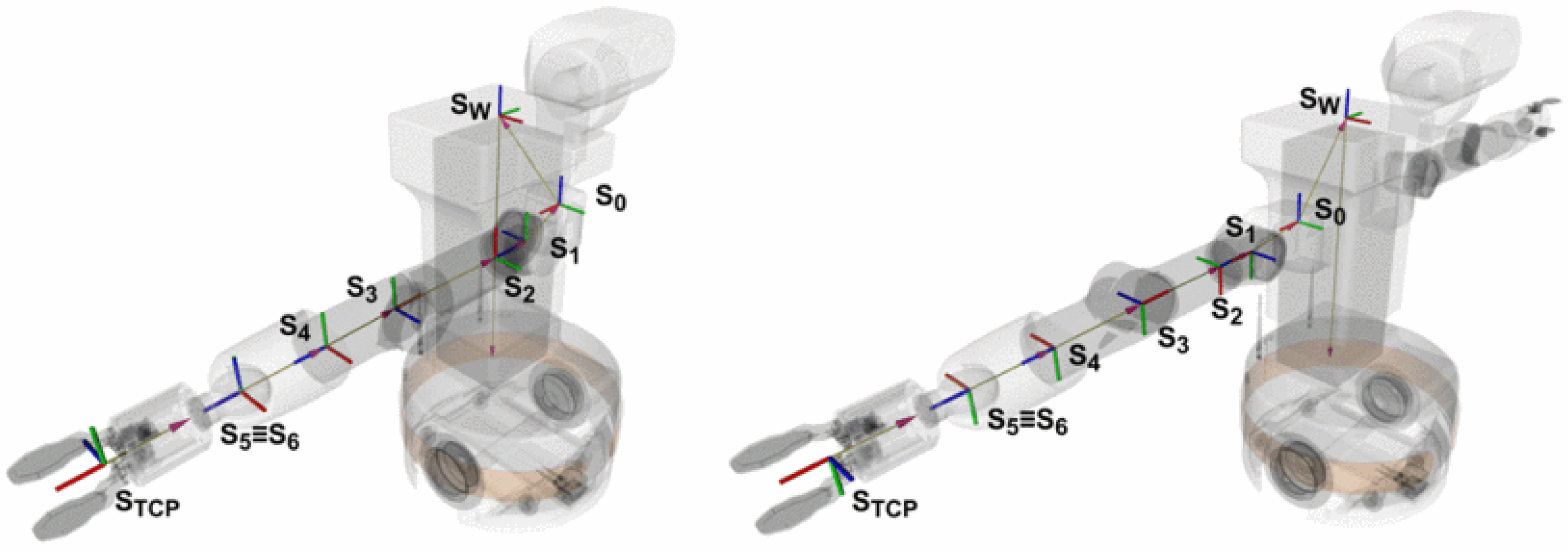
Figure 2.
Denavit–Hartenberg coordinate frames for TIAGo (left) and TIAGo++ right arm (right) [
25]. The color of the axes follows the usual convention (red for
x, green for
y and blue for
z).
Figure 2.
Denavit–Hartenberg coordinate frames for TIAGo (left) and TIAGo++ right arm (right) [
25]. The color of the axes follows the usual convention (red for
x, green for
y and blue for
z).
Figure 3.
Representation of the robot model in the Gazebo robot simulator (left) and pykin (right).
Figure 3.
Representation of the robot model in the Gazebo robot simulator (left) and pykin (right).
Figure 4.
SimpleMlp: Fully connected feed-forward Deep Neural Network for learning Inverse Kinematics. The input size is set for a 3D Cartesian position and quaternion orientation, the hidden layer contains 160 neurons, and the output size corresponds to the 7 DOFs of TIAGo’s arm.
Figure 4.
SimpleMlp: Fully connected feed-forward Deep Neural Network for learning Inverse Kinematics. The input size is set for a 3D Cartesian position and quaternion orientation, the hidden layer contains 160 neurons, and the output size corresponds to the 7 DOFs of TIAGo’s arm.
Figure 5.
DeepMlp: Fully connected feed-forward Deep Neural Network for learning Inverse Kinematics. The input size is set for a 3D Cartesian position and quaternion orientation, it contains 80 hidden layers of 128/256 neurons, and the output size corresponds to the 7 DOFs of TIAGo’s arm.
Figure 5.
DeepMlp: Fully connected feed-forward Deep Neural Network for learning Inverse Kinematics. The input size is set for a 3D Cartesian position and quaternion orientation, it contains 80 hidden layers of 128/256 neurons, and the output size corresponds to the 7 DOFs of TIAGo’s arm.
Figure 6.
SubnetMlp: Fully connected feed-forward Deep Neural Network for learning Inverse Kinematics. It contains a subnet with one hidden layer for each joint.
Figure 6.
SubnetMlp: Fully connected feed-forward Deep Neural Network for learning Inverse Kinematics. It contains a subnet with one hidden layer for each joint.
Figure 7.
CNN: Convolutional Deep Neural Network for learning Inverse Kinematics. It contains 2 convolutional layers, 1 pooling layer, and fully connected layers.
Figure 7.
CNN: Convolutional Deep Neural Network for learning Inverse Kinematics. It contains 2 convolutional layers, 1 pooling layer, and fully connected layers.
Figure 8.
SimpleRnn: Recurrent Neural Network for learning Inverse Kinematics. It contains one hidden recurrent layer.
Figure 8.
SimpleRnn: Recurrent Neural Network for learning Inverse Kinematics. It contains one hidden recurrent layer.
Figure 9.
LSTM: Recurrent Deep Neural Network for learning Inverse Kinematics. It contains LSTM layers, dense layers, and dropout layers in between.
Figure 9.
LSTM: Recurrent Deep Neural Network for learning Inverse Kinematics. It contains LSTM layers, dense layers, and dropout layers in between.
Figure 10.
Test run on sets of 10,000 non-normalized samples, using different representations for the orientation. The first plot depicts the validation loss given by the mean squared error.
Figure 10.
Test run on sets of 10,000 non-normalized samples, using different representations for the orientation. The first plot depicts the validation loss given by the mean squared error.
Figure 11.
Test run on the same set of 10,000 samples, using different preprocessing normalization techniques.
Figure 11.
Test run on the same set of 10,000 samples, using different preprocessing normalization techniques.
Figure 12.
Test run on the same set of 100,000 normalized samples, using different models. In the first image, the y-axis is limited to 1.7 to reduce the effects of the SubnetMlp outliers.
Figure 12.
Test run on the same set of 100,000 normalized samples, using different models. In the first image, the y-axis is limited to 1.7 to reduce the effects of the SubnetMlp outliers.
Figure 13.
Comparison of the different metrics for the SimpleMlp model trained with a dataset with and without curriculums.
Figure 13.
Comparison of the different metrics for the SimpleMlp model trained with a dataset with and without curriculums.
Figure 14.
TIAGo robot placed inside the motion capture structure.
Figure 14.
TIAGo robot placed inside the motion capture structure.
Figure 15.
Motion capture markers as detected by the system.
Figure 15.
Motion capture markers as detected by the system.
Table 1.
Denavit–Hartenberg parameters for TIAGo and TIAGo++ right arm [
25].
Table 1.
Denavit–Hartenberg parameters for TIAGo and TIAGo++ right arm [
25].
| DOF | | D | A | | | D | A | |
|---|
| 1 | 0 | −31 | 125 | | 0 | −31 | 125 | |
| 2 | | −21 | 0 | | | −21 | 0 | |
| 3 | 0 | −311.5 | −20 | | 0 | −311.5 | −20 | |
| 4 | 0 | 0 | 20 | | 0 | 0 | 20 | |
| 5 | | 312 | 0 | | | 312 | 0 | |
| 6 | 0 | 0 | 0 | | 0 | 0 | 0 | |
| 7 | 0 | 46 | 0 | 0 | 0 | 46 | 0 | 0 |
Table 2.
Comparison of the different metrics obtained on testing for the SimpleMlp model after training with different orientation representations on a dataset with 10,000 non-normalized samples.
Table 2.
Comparison of the different metrics obtained on testing for the SimpleMlp model after training with different orientation representations on a dataset with 10,000 non-normalized samples.
| Orientation | MSE | Position Error | Orientation Error |
|---|
| Quaternion | 0.5964 | 0.4847 | 0.6157 |
| Rotation matrix | 0.7476 | 0.4855 | 0.7356 |
| None | 0.8269 | 0.4433 | 0.8954 |
Table 3.
Comparison of the different metrics obtained on testing for the SimpleMlp model after training with different normalization techniques on the same dataset with 10,000 samples.
Table 3.
Comparison of the different metrics obtained on testing for the SimpleMlp model after training with different normalization techniques on the same dataset with 10,000 samples.
| Normalization | MSE | Position Error | Orientation Error |
|---|
| None | 0.6163 | 0.4770 | 0.6295 |
| Standardization | 0.7297 | 0.3351 | 0.7630 |
| Min–max | 0.3111 | 0.4740 | 0.9439 |
| Max–absolute | 0.1074 | 0.1750 | 0.3352 |
| Robust scaling | 0.1292 | 0.1470 | 0.3081 |
Table 4.
Comparison of the different metrics for each model, obtained from the test set split from the same 100,000 samples dataset, normalized using robust scaling.
Table 4.
Comparison of the different metrics for each model, obtained from the test set split from the same 100,000 samples dataset, normalized using robust scaling.
| Model | MSE | Position Error | Orientation Error |
|---|
| SimpleMlp | 0.1286 | 0.1395 | 0.2992 |
| DeepMlp | 1.4451 | 0.7872 | 1.0508 |
| SubnetMlp | 0.1155 | 0.1429 | 0.2949 |
| CNN | 1.3380 | 0.9288 | 1.0193 |
| SimpleRnn | 0.1308 | 0.1468 | 0.3048 |
| LSTM | 0.3578 | 0.5711 | 0.9405 |
Table 5.
Comparison of the different metrics for the SimpleMlp model trained with a dataset with and without curriculums.
Table 5.
Comparison of the different metrics for the SimpleMlp model trained with a dataset with and without curriculums.
| Curriculum Division | Threshold | MSE | Position Error | Orientation Error | Time |
|---|
| None | No | 0.1286 | 0.1395 | 0.2992 | 19 m 39 s |
| By equal distance | No | 0.1212 | 0.1351 | 0.2753 | 17 m 34 s |
| By equal distance | Yes | 0.1232 | 0.1400 | 0.2764 | 17 m 17 s |
| By equal number of samples | No | 0.1222 | 0.1443 | 0.2889 | 16 m 47 s |
| By equal number of samples | Yes | 0.1229 | 0.1432 | 0.2745 | 17 m 1 s |
Table 6.
Comparison of the different metrics for the SubnetMlp model and classic solvers.
Table 6.
Comparison of the different metrics for the SubnetMlp model and classic solvers.
| Method | MSE | Failures | Time |
|---|
| SubnetMlp | 0.6901 | 0 | 0.91 s |
| Newton–Raphson | 2.9338 | 9456 | 27.76 s |
| Levenberg–Marquardt | 27,560.6995 | 9416 | 12.89 s |
Table 7.
Example of the values extracted after the sim2real experiment. Values are in meters.
Table 7.
Example of the values extracted after the sim2real experiment. Values are in meters.
| | Joint Target | Joint Reached | | FK (Joint Targets) | FK (Joint Reached) |
|---|
| 1.3630 | 1.3631 | X | −0.1582 | −0.1580 |
| 0.4001 | 0.4002 | Y | 0.1291 | 0.1290 |
| −0.5982 | −0.5982 | Z | 0.5531 | 0.5530 |
| 0.1366 | 0.1362 | x | −0.2670 | −0.0805 |
| 0.7321 | 0.732 | y | −0.3292 | 0.3326 |
| 0.3664 | 0.3666 | z | −0.7417 | −0.1420 |
| 1.5843 | 1.5844 | w | 0.5196 | 0.9288 |
Table 8.
Example of the values extracted after the sim2real experiment. Values are in meters.
Table 8.
Example of the values extracted after the sim2real experiment. Values are in meters.
| | Joint Reached | | FK (Joint Reached) | Motion Capture Pose |
|---|
| 1.3631 | X | −0.1580 | −0.2065 |
| 0.4002 | Y | 0.1290 | 0.0203 |
| −0.5982 | Z | 0.5530 | 0.5239 |
| 0.1362 | x | −0.0805 | 0.7464 |
| 0.732 | y | 0.3326 | −0.6497 |
| 0.3666 | z | −0.1420 | −0.1098 |
| 1.5844 | w | 0.9288 | −0.0922 |
Table 9.
Final errors for sim2real experiment.
Table 9.
Final errors for sim2real experiment.
| | Mean Position Error | Standard Deviation | Mean Orientation Error | Standard Deviation |
|---|
| Error 1 | 0.000093 | 0.000061 | 1.3049 | 0.3609 |
| Error 2 | 0.1382 | 0.0733 | 1.4296 | 0.2276 |
| Global | 0.1382 | 0.0733 | 1.2765 | 0.3430 |
| Disclaimer/Publisher’s Note: The statements, opinions and data contained in all publications are solely those of the individual author(s) and contributor(s) and not of MDPI and/or the editor(s). MDPI and/or the editor(s) disclaim responsibility for any injury to people or property resulting from any ideas, methods, instructions or products referred to in the content. |
© 2025 by the authors. Licensee MDPI, Basel, Switzerland. This article is an open access article distributed under the terms and conditions of the Creative Commons Attribution (CC BY) license (https://creativecommons.org/licenses/by/4.0/).


