


The Design, Creation, Implementation, and Study of a New Dataset Suitable for Non-Intrusive Load Monitoring


Abstract
1. Introduction
- Robust and scalable solutions: Many algorithms perform well in laboratory settings but fail in real-world applications. This is due to the need to adapt to different conditions and usage patterns in the real world [19];
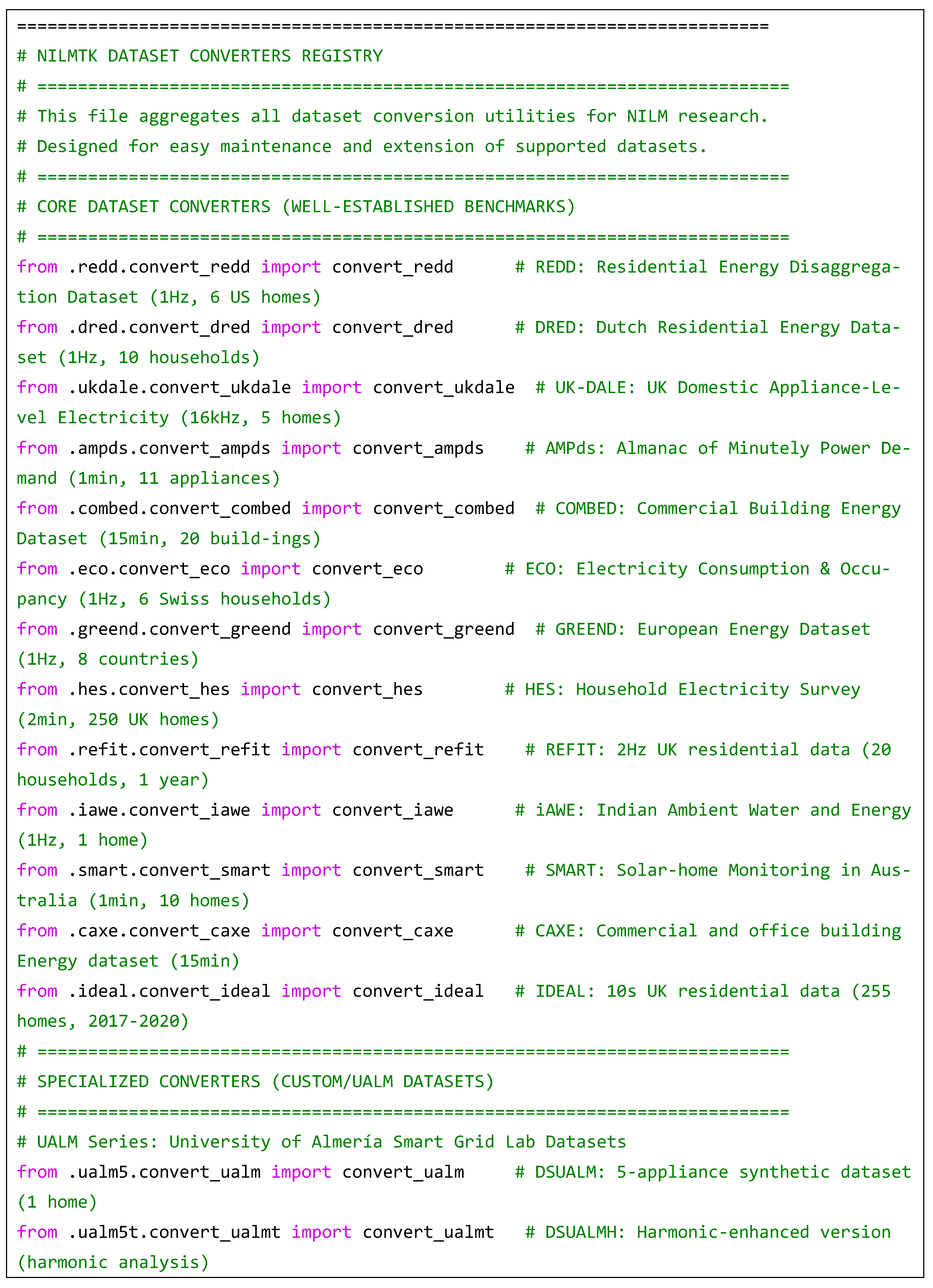
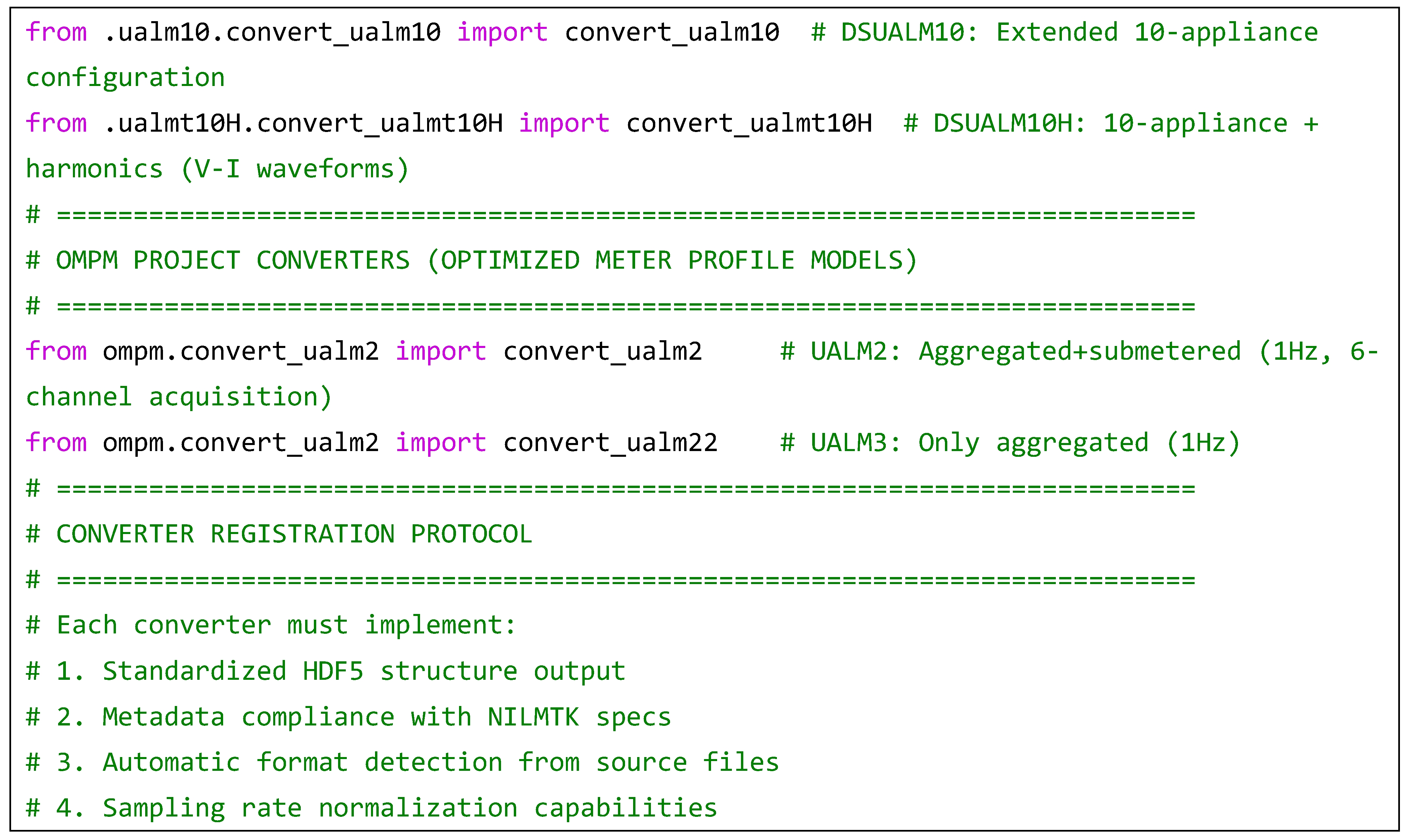
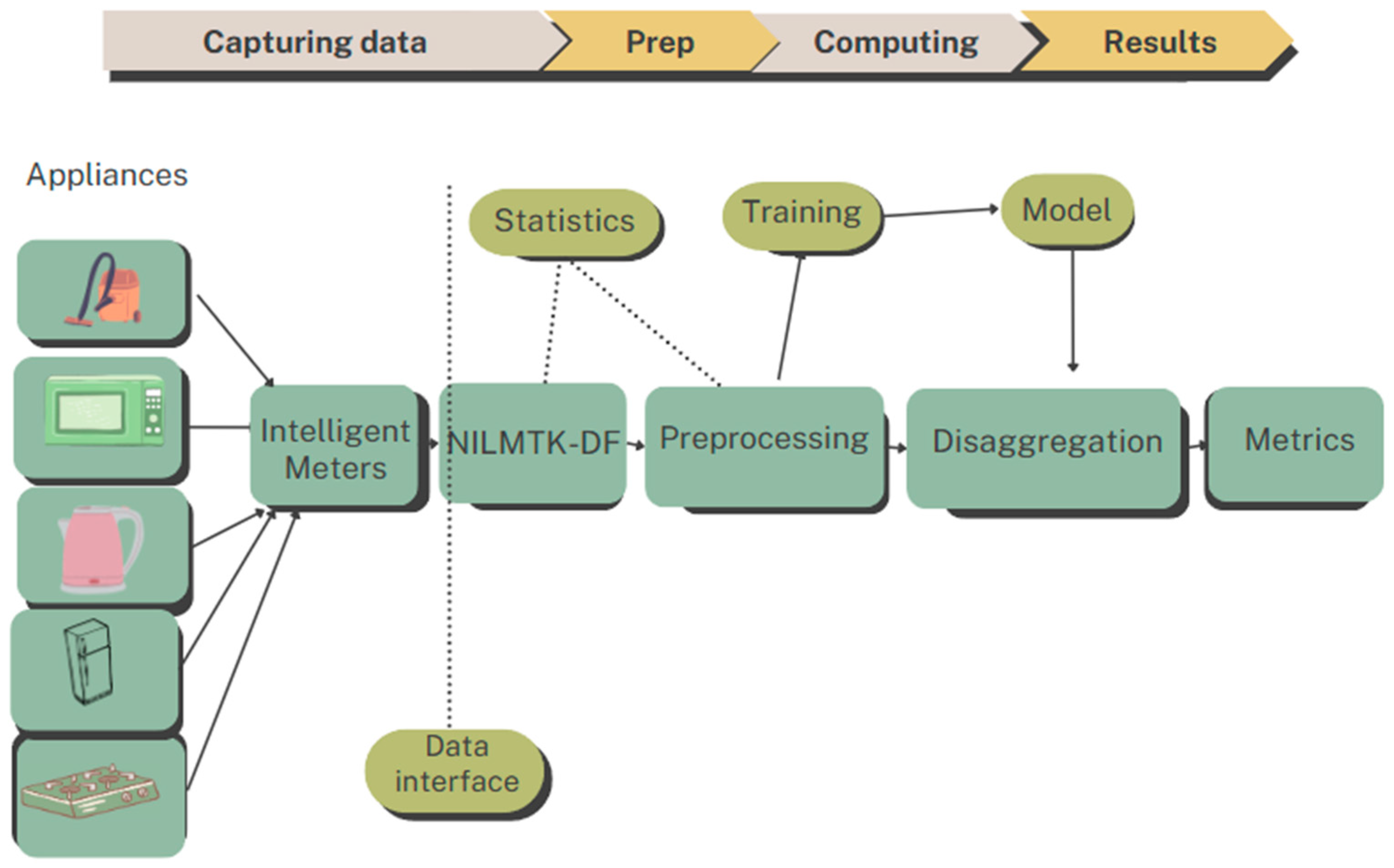
2. NILMTK
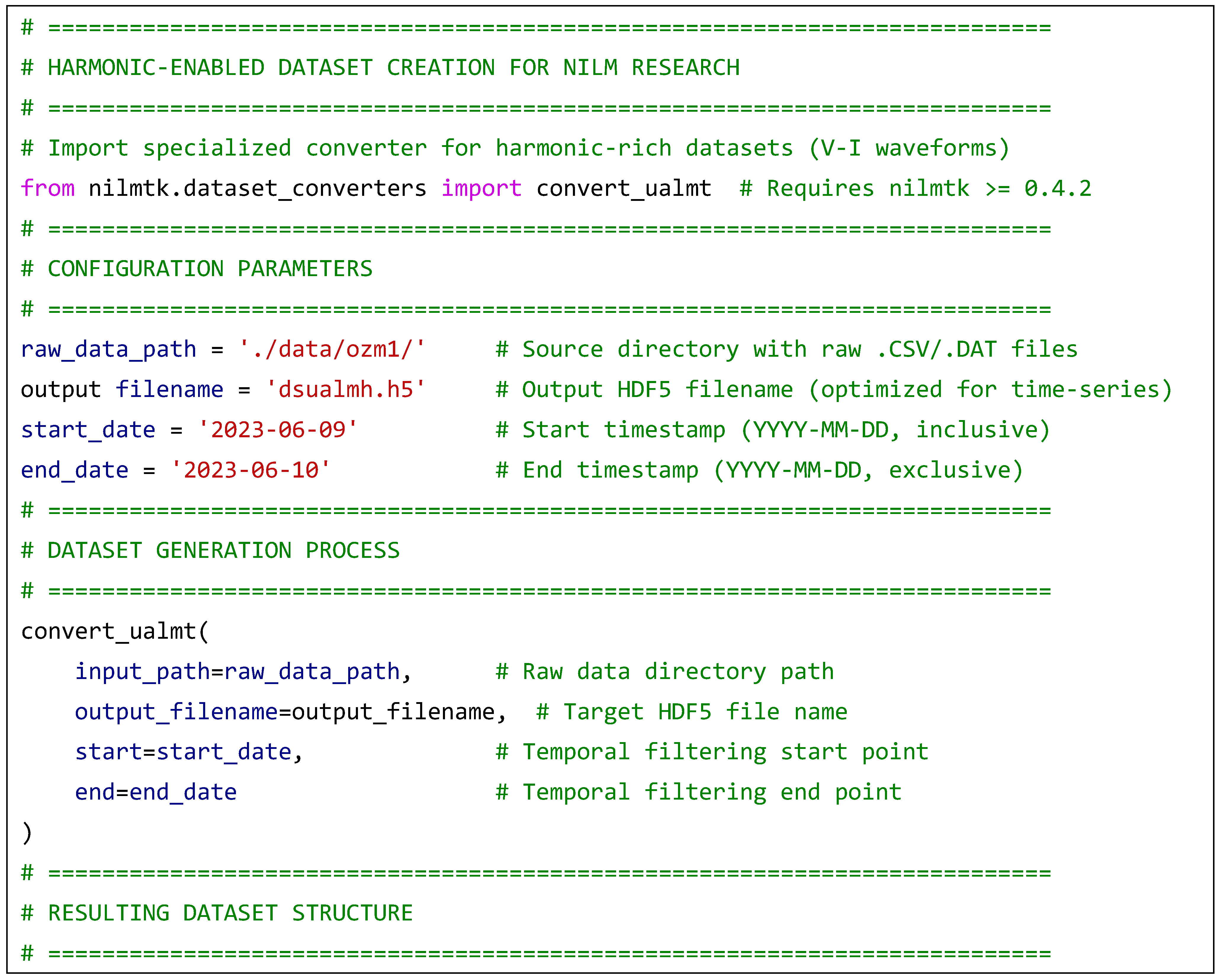
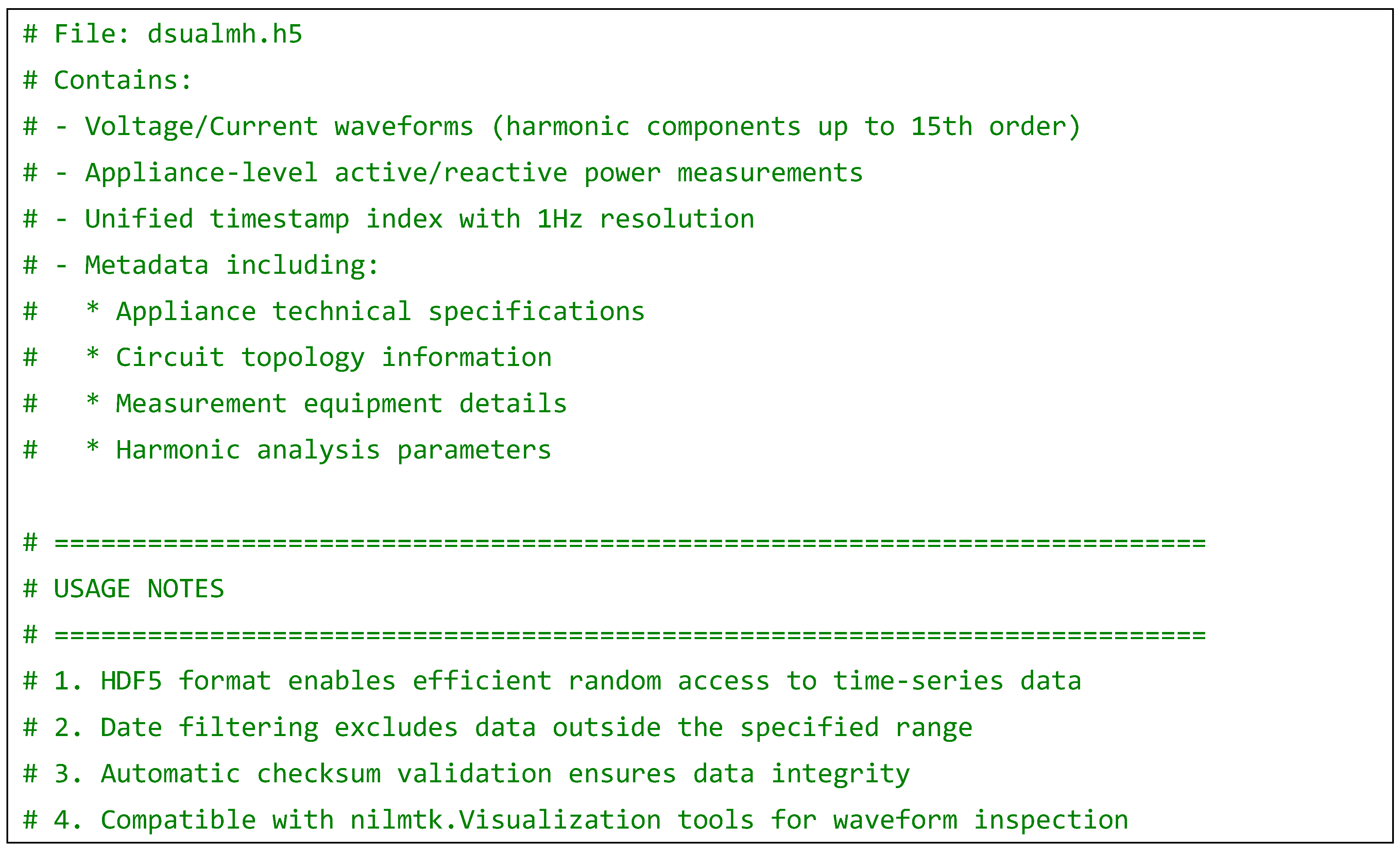
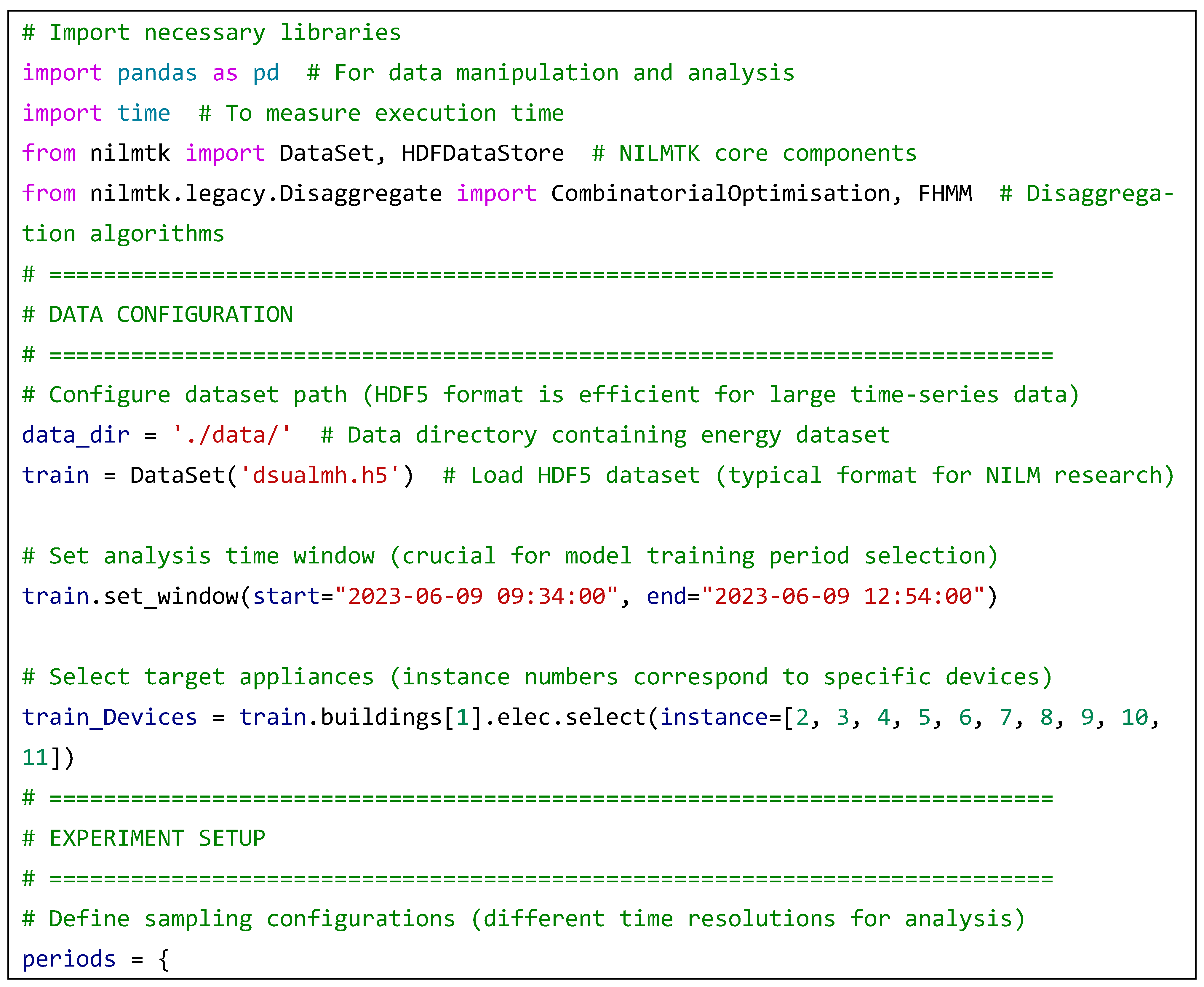
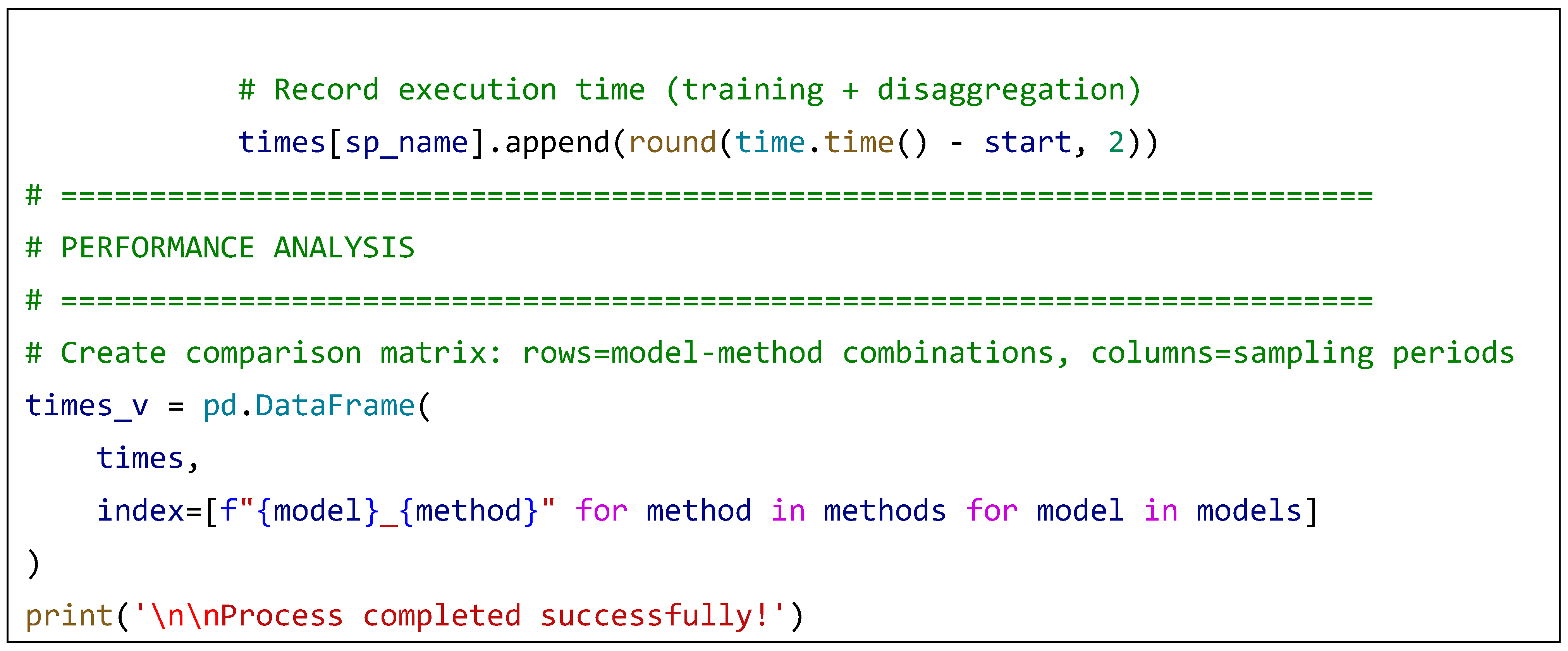
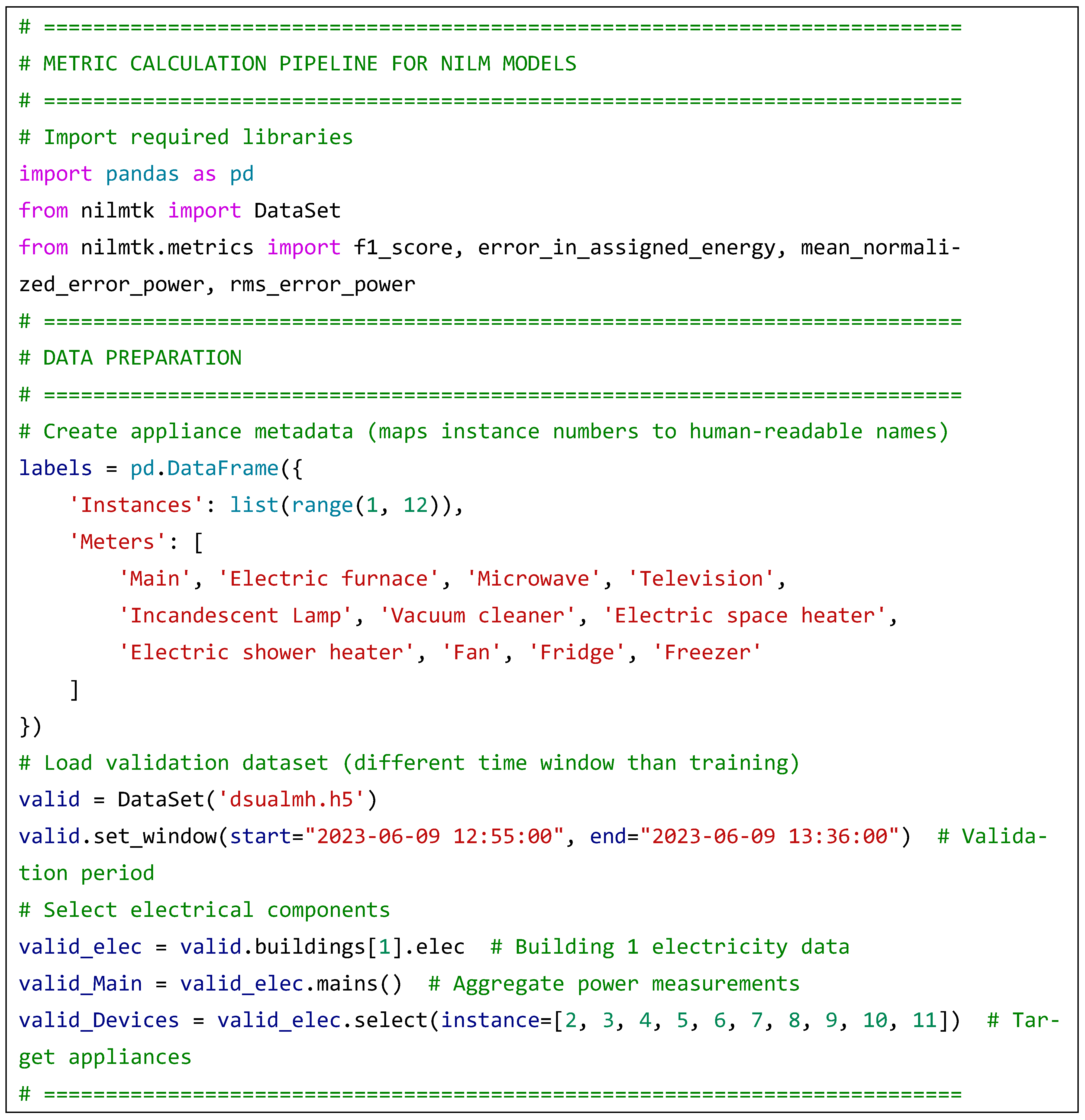
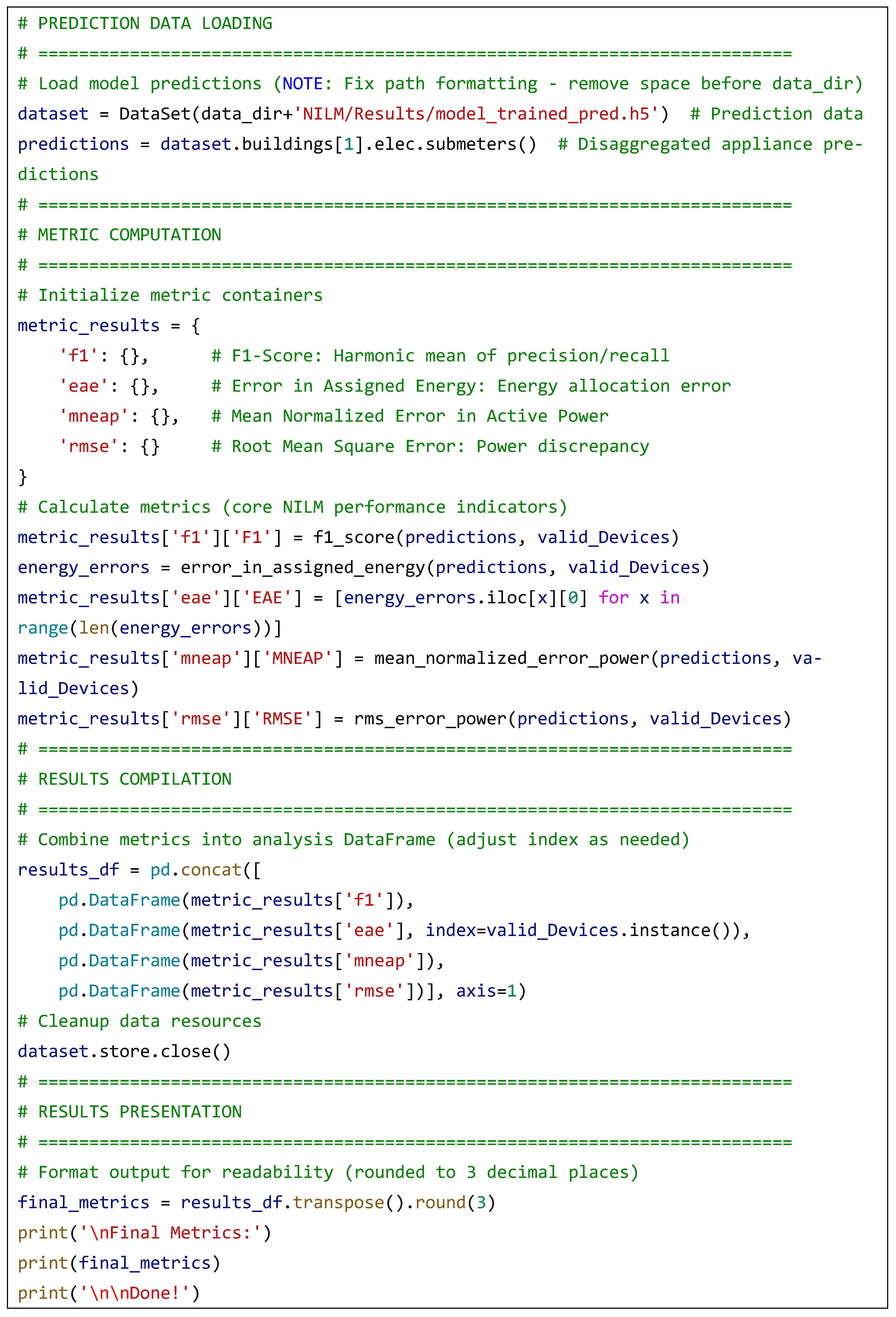
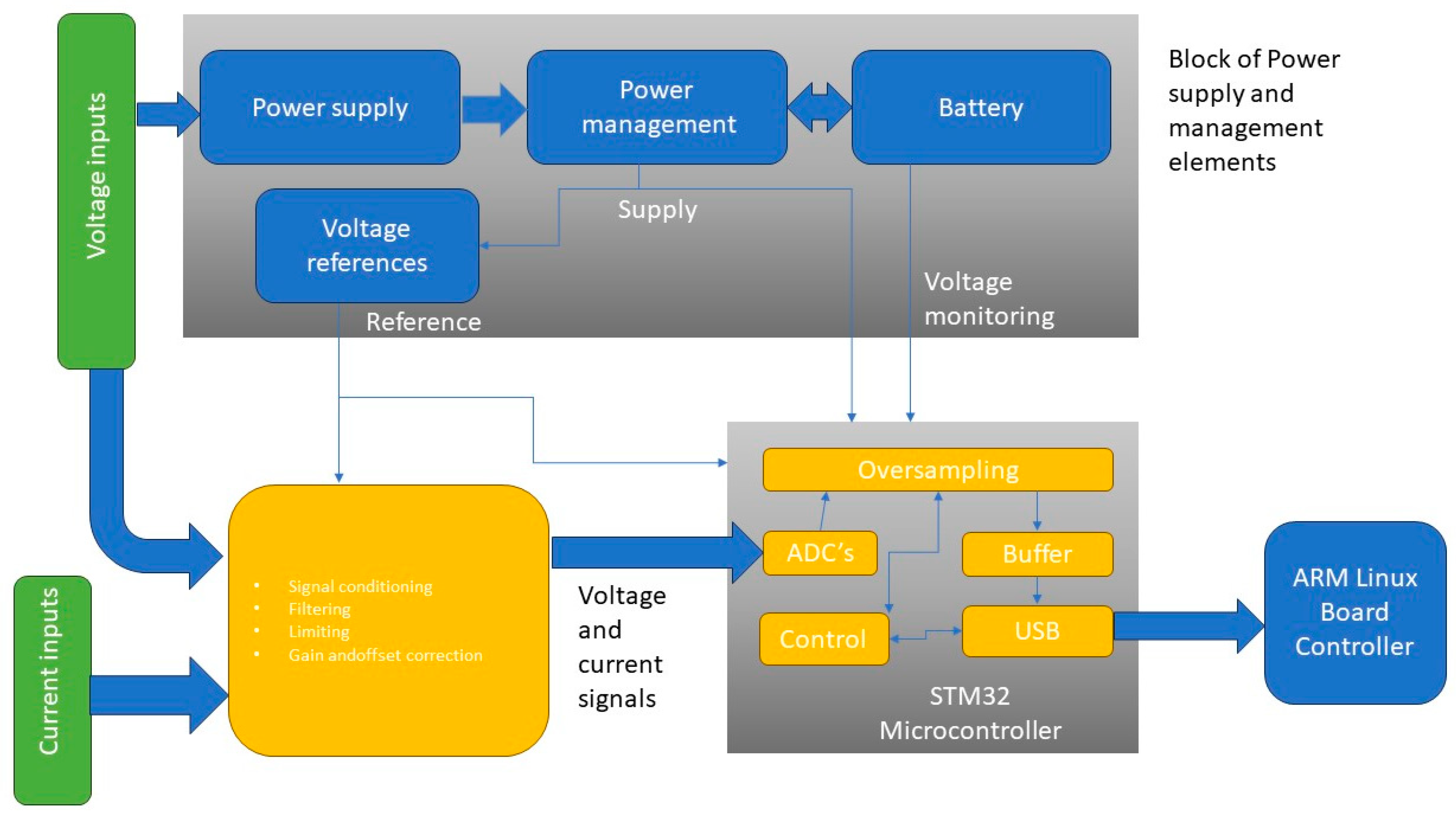
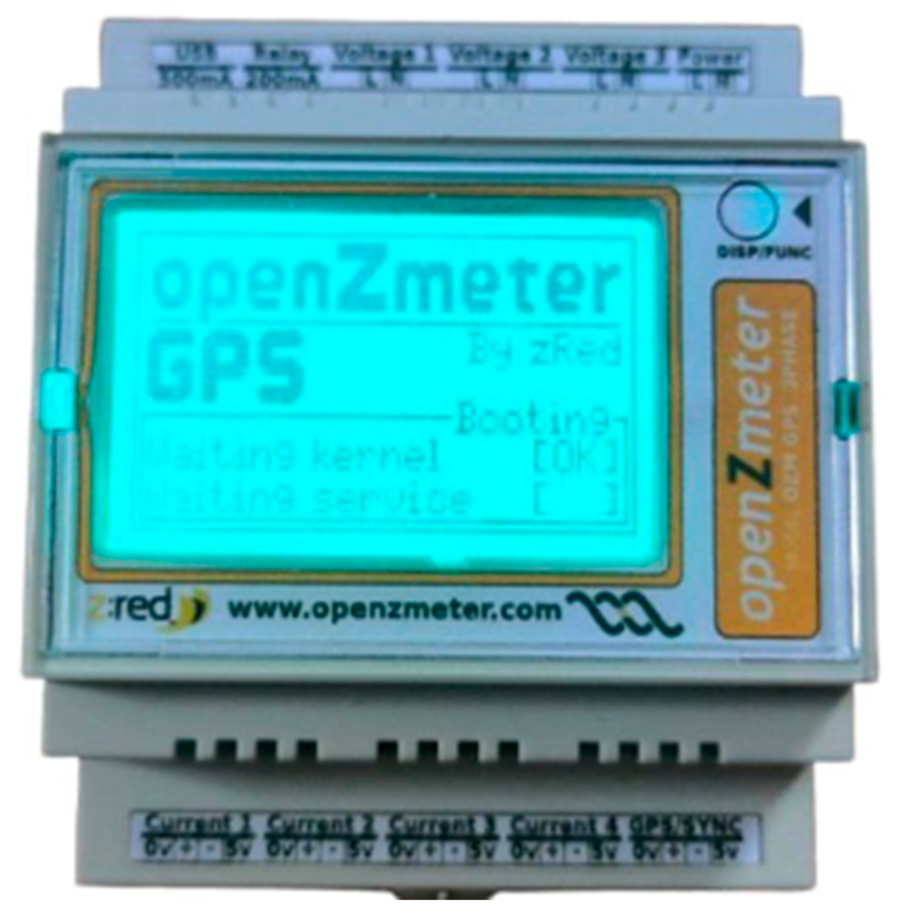
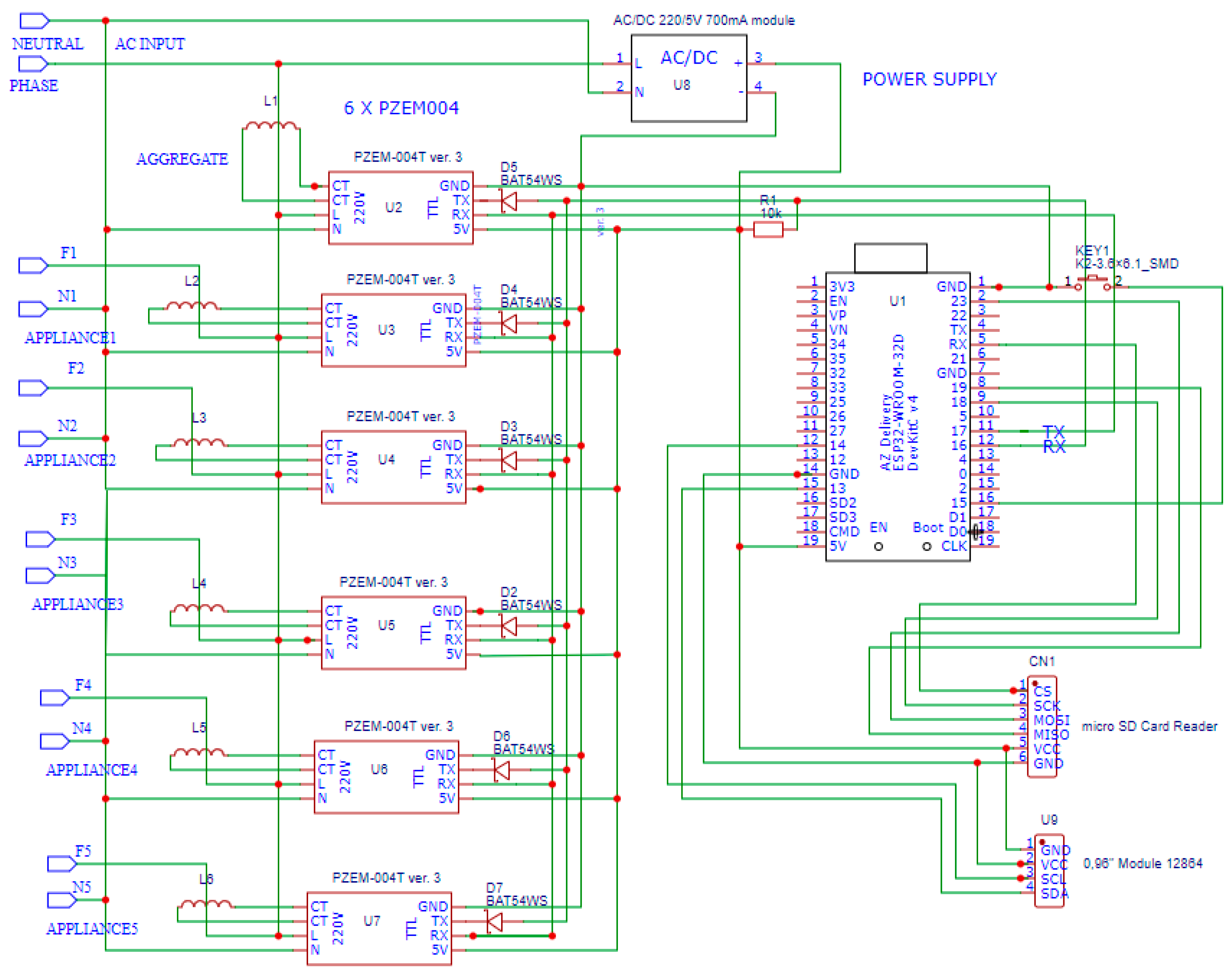
3. Materials and Methods
4. Results and Discussion
4.1. Metrics Obtained from the Different Datasets Generated with Open Hardware
4.1.1. DSUALM and DSUALMH
4.1.2. UALM2
4.1.3. DSUALM10H and DSUALM10
4.2. Comparative Performance Between Datasets
4.2.1. F1-Score
4.2.2. EAE
4.2.3. MNEAP
4.2.4. RMSE
4.2.5. The Summary of the Main Findings
5. Conclusions
6. Limitations and Future Directions
Author Contributions
Funding
Institutional Review Board Statement
Informed Consent Statement
Data Availability Statement
Conflicts of Interest
Abbreviations
| CO | Combinatorial Optimization |
| DAE | Denoising Autoencoder |
| DSUALM | Dataset of the University of Almeria |
| DSUALMH | Dataset of the University of Almeria with harmonics |
| DSUALM10 | Dataset of the University of Almeria 10 appliances |
| DSUALM10H | Dataset of the University of Almeria 10 appliances with harmonics |
| FHMM | Factorial Hidden Markov Model |
| MAE | Mean Absolute Error |
| NDE | Normalized Disaggregation Error |
| NILM | Non-Intrusive Load Monitoring |
| OMPM | Open Multi Power Meter |
| oZm | OpenZmeter |
| RMSE | Root Mean Squared Error |
| RNN | Recurrent Neural Network |
| UAL | University of Almeria |
| UALM2 | University of Almeria Dataset 2 |
| WindowGRU | Windowed Gated Recurrent Unit |
Appendix A

References
- Francou, J.; Calogine, D.; Chau, O.; David, M.; Lauret, P. Expanding Variety of Non-Intrusive Load Monitoring Training Data: Introducing and Benchmarking a Novel Data Augmentation Technique. Sustain. Energy Grids Netw. 2023, 35, 101142. [Google Scholar] [CrossRef]
- Aydin, E.; Brounen, D.; Kok, N. Information Provision and Energy Consumption: Evidence from a Field Experiment. Energy Econ. 2018, 71, 403–410. [Google Scholar] [CrossRef]
- Hart, G.W. Nonintrusive Appliance Load Monitoring. Proc. IEEE 1992, 80, 1870–1891. [Google Scholar] [CrossRef]
- Kelly, J.; Knottenbelt, W. Neural NILM: Deep Neural Networks Applied to Energy Disaggregation. In Proceedings of the BuildSys 2015—Proceedings of the 2nd ACM International Conference on Embedded Systems for Energy-Efficient Built, Seoul, Republic of Korea, 4 November 2015; Association for Computing Machinery, Inc.: New York, NY, USA; pp. 55–64. [Google Scholar]
- Holweger, J.; Dorokhova, M.; Bloch, L.; Ballif, C.; Wyrsch, N. Unsupervised Algorithm for Disaggregating Low-Sampling-Rate Electricity Consumption of Households. Sustain. Energy Grids Netw. 2019, 19, 100244. [Google Scholar] [CrossRef]
- Shin, C.; Rho, S.; Lee, H.; Rhee, W. Data Requirements for Applying Machine Learning to Energy Disaggregation. Energies 2019, 12, 1696. [Google Scholar] [CrossRef]
- Çavdar, I.H.; Faryad, V. New Design of a Supervised Energy Disaggregation Model Based on the Deep Neural Network for a Smart Grid. Energes 2019, 12, 1217. [Google Scholar] [CrossRef]
- Shabbir, N.; Vassiljeva, K.; Nourollahi Hokmabad, H.; Husev, O.; Petlenkov, E.; Belikov, J. Comparative Analysis of Machine Learning Techniques for Non-Intrusive Load Monitoring. Electronics 2024, 13, 1420. [Google Scholar] [CrossRef]
- Irani Azad, M.; Rajabi, R.; Estebsari, A. Nonintrusive Load Monitoring (NILM) Using a Deep Learning Model with a Transformer-Based Attention Mechanism and Temporal Pooling. Electronics 2024, 13, 407. [Google Scholar] [CrossRef]
- Zeng, W.; Han, Z.; Xie, Y.; Liang, R.; Bao, Y. Non-Intrusive Load Monitoring through Coupling Sequence Matrix Reconstruction and Cross Stage Partial Network. Measurement 2023, 220, 113358. [Google Scholar] [CrossRef]
- Athanasiadis, C.; Doukas, D.; Papadopoulos, T.; Chrysopoulos, A. A Scalable Real-Time Non-Intrusive Load Monitoring System for the Estimation of Household Appliance Power Consumption. Energies 2021, 14, 767. [Google Scholar] [CrossRef]
- Yang, C.C.; Soh, C.S.; Yap, V.V. A Non-Intrusive Appliance Load Monitoring for Efficient Energy Consumption Based on Naive Bayes Classifier. Sustain. Comput. Inform. Syst. 2017, 14, 34–42. [Google Scholar] [CrossRef]
- Yan, L.; Tian, W.; Wang, H.; Hao, X.; Li, Z. Robust Event Detection for Residential Load Disaggregation. Appl. Energy 2023, 331, 120339. [Google Scholar] [CrossRef]
- Rafiq, H.; Manandhar, P.; Rodriguez-Ubinas, E.; Ahmed Qureshi, O.; Palpanas, T. A Review of Current Methods and Challenges of Advanced Deep Learning-Based Non-Intrusive Load Monitoring (NILM) in Residential Context. Energy Build 2024, 305, 113890. [Google Scholar] [CrossRef]
- Souza, J. Non-Intrusive Load Monitoring (NILM): An Introduction and Practical Example. Available online: https://www.linkedin.com/pulse/non-intrusive-load-monitoring-nilm-introduction-practical-souza-rpy4f/ (accessed on 11 March 2025).
- Parson, O.; Fisher, G.; Hersey, A.; Batra, N.; Kelly, J.; Singh, A.; Knottenbelt, W.; Rogers, A. Dataport and NILMTK: A Building Data Set Designed for Non-Intrusive Load Monitoring. In Proceedings of the 2015 IEEE Global Conference on Signal and Information Processing (GlobalSIP), Orlando, FL, USA, 14–16 December 2015; IEEE: Piscataway, NJ, USA. [Google Scholar]
- Liu, Q.; Lu, M.; Liu, X.; Linge, N. Non-Intrusive Load Monitoring and Its Challenges in a NILM System Framework. Int. J. High Perform. Comput. Netw. 2019, 14, 102–111. [Google Scholar] [CrossRef]
- Vavouris, A.; Garside, B.; Stankovic, L.; Stankovic, V. Low-Frequency Non-Intrusive Load Monitoring of Electric Vehicles in Houses with Solar Generation: Generalisability and Transferability. Energies 2022, 15, 2200. [Google Scholar] [CrossRef]
- Sykiotis, S.; Kaselimi, M.; Doulamis, A.; Doulamis, N. Electricity: An Efficient Transformer for Non-Intrusive Load Monitoring. Sensors 2022, 22, 2926. [Google Scholar] [CrossRef]
- Lakshmi Ravi, D. Non-Intrusive Load Monitoring (NILM): A Comprehensive Review. Int. J. Innov. Res. Technol. 2024, 11, 853–858. [Google Scholar]
- Nipun, B.; Jack, K.; Oliver, P.; Haimonti, D.; William, K. NILMTK: An Open Source Toolkit for Non-Intrusive Load Monitoring. In Proceedings of the 5th International Conference on Future Energy Systems, Cambridge, UK, 11–13 June 2014. [Google Scholar] [CrossRef]
- Makonin, S.; Popowich, F. Nonintrusive Load Monitoring (NILM) Performance Evaluation. Energy Effic. 2015, 8, 809–814. [Google Scholar] [CrossRef]
- Kukunuri, R.; Batra, N.; Pandey, A.; Malakar, R.; Kumar, R.; Krystalakos, O.; Zhong, M.; Meira, P.; Parson, O. NILMTK-Contrib: Towards Reproducible State-of-the-Art Energy Disaggregation. In Proceedings of the 6th ACM International Conference on Systems for Energy-Efficient Buildings, Cities, and Transportation, New York, NY, USA, 13–14 November 2019. [Google Scholar]
- Kolter, J.Z.; Johnson, M.J. REDD: A Public Data Set for Energy Disaggregation Research. In Proceedings of the 1st KDD Workshop on Data Mining Applications in Sustainability, San Diego, CA, USA, 21 August 2011. [Google Scholar]
- Kelly, J.; Knottenbelt, W. The UK-DALE Dataset, Domestic Appliance-Level Electricity Demand and Whole-House Demand from Five UK Homes. Sci. Data 2015, 2, 150007. [Google Scholar] [CrossRef]
- Beckel, C.; Kleiminger, W.; Cicchetti, R.; Staake, T.; Santini, S. The ECO Data Set and the Performance of Non-Intrusive Load Monitoring Algorithms. In Proceedings of the BuildSys 2014—Proceedings of the 1st ACM Conference on Embedded Systems for Energy-Efficient Buildings, Memphis, TN, USA, 3 November 2014; Association for Computing Machinery: New York, NY, USA; pp. 80–89. [Google Scholar]
- Certification, L. Pecan Street Dataport. Available online: https://www.pecanstreet.org/dataport/ (accessed on 17 June 2025).
- Berrettoni, G.; Ferrigno Fabrizio Marignetti, L. Resilience of the Italian Electricity Grid: Objectives and Future Challenges; University of Cassino: Cassino, Italy, 2024. [Google Scholar]
- Bonfigli, R.; Principi, E.; Fagiani, M.; Severini, M.; Squartini, S.; Piazza, F. Non-Intrusive Load Monitoring by Using Active and Reactive Power in Additive Factorial Hidden Markov Models. Appl. Energy 2017, 208, 1590–1607. [Google Scholar] [CrossRef]
- Gawin, B.; Małkowski, R.; Rink, R. Will NILM Technology Replace Multi-Meter Telemetry Systems for Monitoring Electricity Consumption? Energies 2023, 16, 2275. [Google Scholar] [CrossRef]
- Rodríguez-Navarro, C.; Portillo, F.; Martínez, F.; Manzano-Agugliaro, F.; Alcayde, A. Development and Application of an Open Power Meter Suitable for NILM. Inventions 2023, 9, 2. [Google Scholar] [CrossRef]
- Rodriguez-Navarro, C. Datasets of Almeria University. Available online: https://zenodo.org/records/13739113 (accessed on 27 February 2025).
- Rodriguez-Navarro, C. DSUALMH. Available online: https://zenodo.org/records/13739563 (accessed on 17 June 2025).
- Viciana, E.; Alcayde, A.; Montoya, F.; Baños, R.; Arrabal-Campos, F.; Zapata-Sierra, A.; Manzano-Agugliaro, F. OpenZmeter: An Efficient Low-Cost Energy Smart Meter and Power Quality Analyzer. Sustainability 2018, 10, 4038. [Google Scholar] [CrossRef]
- Rodriguez_Navarro, C. OMPM. Available online: https://zenodo.org/records/13740059 (accessed on 17 June 2025).
- Rodriguez-Navarro, C. DSUALM10H. Available online: https://zenodo.org/records/13740027 (accessed on 17 June 2025).
- Rodriguez-Navarro, C. Performance Analysis of Nine Disaggregation Algorithms on the DSUALM10 Dataset: A Notebook Study. Available online: https://zenodo.org/records/15575404 (accessed on 17 June 2025).


| Methods | Advantages | Disadvantages | Practical Applications |
|---|---|---|---|
| Traditional models (HMM, FHMM, and decision trees) | Interpretable; requires less training data | Lower accuracy in scenarios with high consumption variability | Used in early NILM implementations, such as energy monitoring systems in research projects like REDD and UK-DALE datasets |
| Neural networks (CNN, RNN, and deep learning) | High accuracy, can capture complex patterns | Require large amounts of data and high computational power | Applied in smart home energy management platforms like Google’s Nest and Sense Energy Monitor |
| Advanced techniques (CSPNet and Coupled Sequence Matrix Reconstruction) | Improved performance by leveraging temporal variations | Still in experimental stages; lack of standardized metrics | Being tested in advanced NILM research for industrial and smart grid applications |
| Edge computing-based NILM | Lower latency, enhanced privacy, and reduced bandwidth usage | Hardware limitations and energy consumption constraints | Used in IoT-enabled smart meters to provide real-time feedback in smart homes and microgrid management |
| MAE (W) | RMSE (W) | F1-Score | NDE | Runtime (s) | ||||||
|---|---|---|---|---|---|---|---|---|---|---|
| Harmonics | No | Yes | No | Yes | No | Yes | No | Yes | No | Yes |
| CO | 457.39 | 455.3 | 511.08 | 510.48 | 0.57 | 0.56 | 108.38 | 107.95 | 1.22 | 1.33 |
| Mean | 387.05 | 241.29 | 389.42 | 242.32 | 0.56 | 0.56 | 108.11 | 54.17 | 0.49 | 0.76 |
| Hart85 | 238.64 | 238.63 | 405.68 | 405.68 | 0.45 | 0.45 | 41.39 | 41.39 | 1.11 | 1.25 |
| FHMM | 14.87 | 13.99 | 25.09 | 25.92 | 0.56 | 0.57 | 2.61 | 2.64 | 0.93 | 1.03 |
| DAE | 4.09 × 10¹² | 3.1 × 10¹² | 1.43 × 10¹³ | 1.08 × 10¹³ | 0.20 | 0.29 | 2.52 × 10¹⁰ | 1.93 × 10¹⁰ | 27.07 | 21.28 |
| RNN | 368.1 | 368.1 | 468.33 | 468.33 | 0.32 | 0.32 | 65.15 | 65.15 | 682.77 | 682.77 |
| Seq2Point | 4.31 × 10¹² | 4.54 × 10¹² | 1.58 × 10¹³ | 1.67 × 10¹³ | 0.03 | 0.28 | 3.00 × 10¹¹ | 1.75 × 10¹¹ | 208.38 | 237.83 |
| Seq2Seq | 3.26 × 10¹² | 3.17 × 10¹² | 1.61 × 10¹³ | 1.30 × 10¹³ | 0.19 | 0.17 | 8.43 × 10¹⁰ | 9.10 × 10¹⁰ | 34.67 | 30.01 |
| WindowGRU | 3.09 × 10¹² | 3.12 × 10¹² | 2.46 × 10¹³ | 2.34 × 10¹³ | 0.30 | 0.33 | 7.34 × 10¹² | 5.23 × 10¹² | 1321.34 | 970.98 |
| Algorithm | MAE (W) | RMSE (W) | F1-Score | NDE | Runtime (s) |
|---|---|---|---|---|---|
| CO | 9.49 | 12.26 | 0.7 | 0.43 | 1.49 |
| Mean | 13.19 | 12.88 | 0.17 | 0.48 | 0.58 |
| FHMM | 12.71 | 15.53 | 0.66 | 0.5 | 1.7 |
| DAE | 4.01 × 10¹² | 2.10 × 10¹³ | 0.2 | 3.54 × 10¹⁰ | 27.07 |
| RNN | 13.36 | 14.53 | 0.17 | 0.51 | 2723.48 |
| Seq2Point | 11.6 | 12.65 | 0.17 | 0.56 | 841.65 |
| Seq2Seq | 6.04 × 10¹¹ | 1.52 × 10¹³ | 0.2 | 9.06 × 10¹⁰ | 34.67 |
| WindowGRU | 8.73 | 10.55 | 0.51 | 0.43 | 3869.17 |
| Algorithm | Harmonics | NDE | F1-Score | RMSE (W) | MAE (W) | Runtime (s) |
|---|---|---|---|---|---|---|
| CO | No | 1.853 | 0.463 | 376.207 | 208.329 | 3.25 |
| Yes | 1.859 | 0.445 | 383.763 | 216.945 | 2.61 | |
| Mean | No | 0.827 | 0.499 | 295.45 | 241.034 | 1.31 |
| Yes | 0.827 | 0.499 | 295.45 | 241.034 | 1.22 | |
| Hart85 | No | 0.92 | 0.114 | 282.7 | 144.046 | 8.54 |
| FHMM | No | 1.101 | 0.419 | 405.841 | 224.72 | 66.31 |
| Yes | 0.984 | 0.39 | 322.955 | 158.119 | 61.76 | |
| DAE | No | 0.743 | 0.529 | 242.217 | 169.454 | 310.57 |
| Yes | 0.736 | 0.522 | 234.881 | 154.166 | 138.07 | |
| RNN | No | 0.652 | 0.593 | 191.057 | 112.596 | 5456.35 |
| Yes | 0.619 | 0.558 | 180.981 | 111.258 | 1880.32 | |
| Seq2Ppoint | No | 0.633 | 0.555 | 189.776 | 111.629 | 1431.18 |
| Yes | 0.629 | 0.528 | 203.484 | 132.55 | 754.77 | |
| Seq2Seq | No | 0.619 | 0.526 | 188.774 | 121.387 | 524.77 |
| Yes | 0.689 | 0.495 | 225.348 | 142.535 | 8613.56 | |
| WindowGRU | No | 0.714 | 0.5 | 232.156 | 150.051 | 6982.46 |
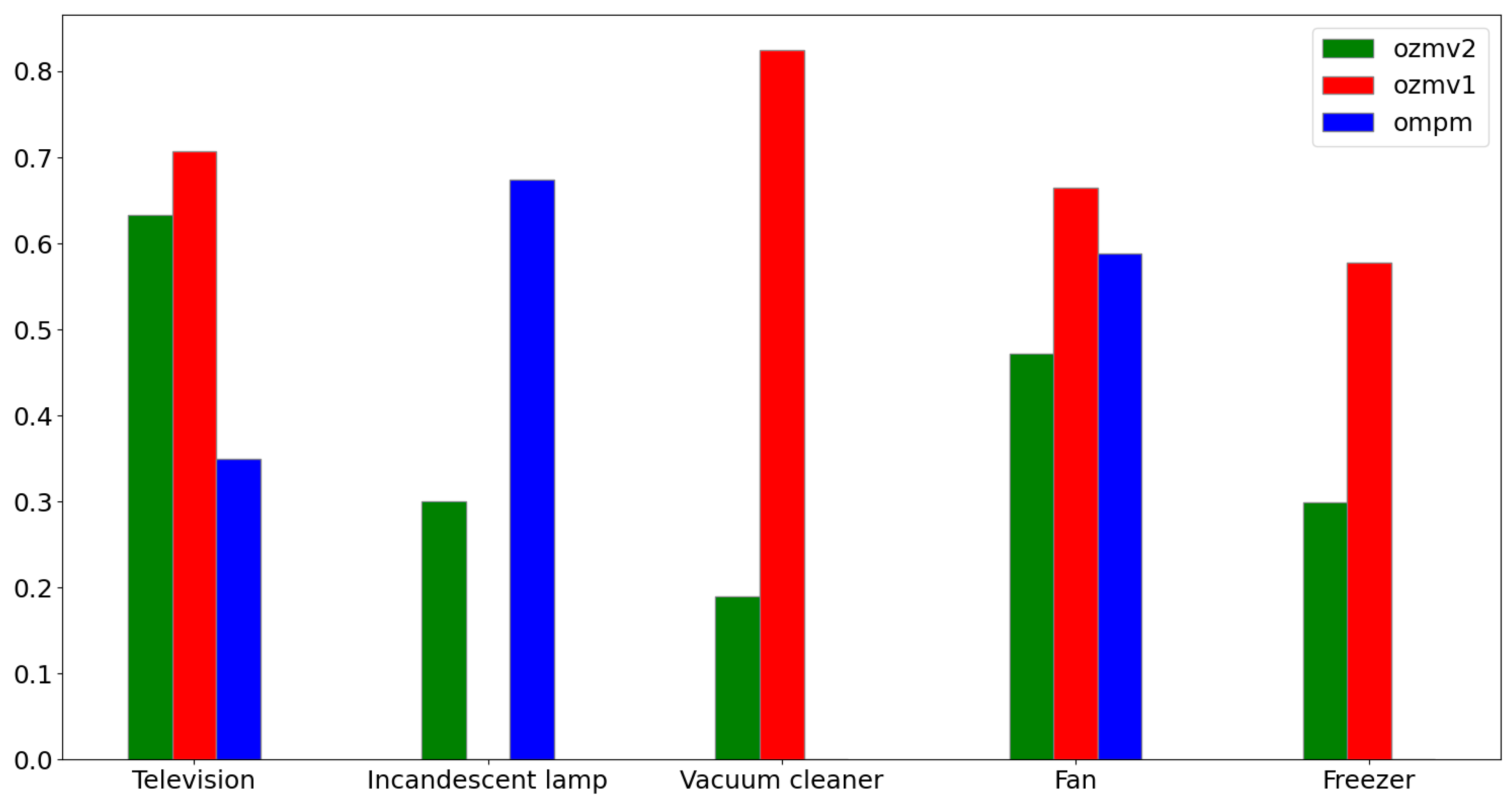
| TV | Lamp | Vac. Cleaner | Fan | Freezer | ||
|---|---|---|---|---|---|---|
| DSUALM10H (oZm v3) | Mean | 0.609 | 0.289 | 0.182 | 0.453 | 0.287 |
| SD | 0.248 | 0.202 | 0.109 | 0.232 | 0.165 | |
| DSUALMH (oZm v1) | Mean | 0.707 | No data | 0.825 | 0.664 | 0.578 |
| SD | 0.154 | No data | 0.125 | 0.128 | 0.126 | |
| UALM2 (OMPM) | Mean | 0.350 | 0.675 | No data | 0.589 | No data |
| SD | 0.275 | 0.254 | No data | 0.254 | No data |
Disclaimer/Publisher’s Note: The statements, opinions and data contained in all publications are solely those of the individual author(s) and contributor(s) and not of MDPI and/or the editor(s). MDPI and/or the editor(s) disclaim responsibility for any injury to people or property resulting from any ideas, methods, instructions or products referred to in the content. |
© 2025 by the authors. Licensee MDPI, Basel, Switzerland. This article is an open access article distributed under the terms and conditions of the Creative Commons Attribution (CC BY) license (https://creativecommons.org/licenses/by/4.0/).
Share and Cite
Rodriguez-Navarro, C.; Portillo, F.; Montoya, F.G.; Alcayde, A. The Design, Creation, Implementation, and Study of a New Dataset Suitable for Non-Intrusive Load Monitoring. Appl. Sci. 2025, 15, 7200. https://doi.org/10.3390/app15137200
Rodriguez-Navarro C, Portillo F, Montoya FG, Alcayde A. The Design, Creation, Implementation, and Study of a New Dataset Suitable for Non-Intrusive Load Monitoring. Applied Sciences. 2025; 15(13):7200. https://doi.org/10.3390/app15137200
Chicago/Turabian StyleRodriguez-Navarro, Carlos, Francisco Portillo, Francisco G. Montoya, and Alfredo Alcayde. 2025. "The Design, Creation, Implementation, and Study of a New Dataset Suitable for Non-Intrusive Load Monitoring" Applied Sciences 15, no. 13: 7200. https://doi.org/10.3390/app15137200
APA StyleRodriguez-Navarro, C., Portillo, F., Montoya, F. G., & Alcayde, A. (2025). The Design, Creation, Implementation, and Study of a New Dataset Suitable for Non-Intrusive Load Monitoring. Applied Sciences, 15(13), 7200. https://doi.org/10.3390/app15137200