A Multi-Scale Unsupervised Feature Extraction Network with Structured Layer-Wise Decomposition

Abstract

Recent developments in deep learning have underscored prizing effective feature extraction in scenarios with limited or unlabeled data. This study introduces a novel unsupervised multi-scale feature extraction framework based on a multi-branch auto-encoder architecture. The proposed method decomposes input images into smooth, detailed and residual components, using variational loss functions to ensure that each branch captures distinct and non-overlapping representations. This decomposition enhances the information richness of input data while preserving its structural integrity, making it especially beneficial for grayscale or low-resolution images. Experimental results on classification and image segmentation tasks show that the proposed method enhances model performance by enriching input representations. Its architecture is scalable and adaptable, making it applicable to a wide range of machine learning tasks beyond image classification and segmentation. These findings highlight the proposed method’s utility as a robust, general-purpose solution for unsupervised feature extraction and multi-scale representation learning.

1. Introduction

In recent years, rapid technological advances have led to a dramatic increase in the volume of accessible data. This surge in data availability has contributed significantly to the development of computer-based systems designed for a wide range of purposes, particularly those that aim to improve human well-being through intelligent decision making, automation, and data-driven optimization. Moreover, the growing abundance of data and the increasing computational power have sped up the progress of artificial intelligence research, especially in deep learning, enhancing its capabilities and enabling its widespread adoption in almost all domains, such as image classification [1,2], denoising [3], object detection [4,5], image segmentation [6,7], decision support systems [8,9], medical imaging [10,11], facial expression recognition [12,13], and remote sensing [14,15]. However, the diverse range of problems addressed by machine learning models often introduces significant complexity and analytical challenges, with model performance still dependent on the quality and relevance of features extracted from raw data. The performance of the model remains dependent on the quality and relevance of the features extracted from the raw data. Moreover, real-world data are rarely perfect and often contain issues such as noise, missing values, or low resolution. Limited data, such as grayscale images, low-quality signals, or abbreviated text, constrains the extractable features in some situations. These limitations make it more difficult for machine learning models to perform, as the quality of input features plays a crucial role in the learning process. Consequently, robust and effective feature extraction is important for improving the performance and success of machine learning models.

Researchers have developed many traditional feature extraction techniques based on mathematical descriptors to derive meaningful information from data. Notable examples include Histogram of Oriented Gradients (HOG) [16], Scale-Invariant Feature Transform (SIFT) [17], Gabor filters [18], Gaussian filters [19], and Local Binary Patterns (LBP) [20]. These methods are computationally efficient and well-suited for scenarios with limited computational resources or small-scale datasets. However, their performance is often constrained by their reliance on manually designed features, which may not generalize well across diverse tasks or data modalities.

With the advent of deep learning, feature extraction has undergone a major transformation. Modern approaches now enable models to automatically learn hierarchical and task-specific representations directly from raw data. Among the most widely used architectures are Convolutional Neural Networks (CNNs) [21], which use convolutional filters to learn spatial features and are widely applied to image, video, and speech data; Transformers [22], which utilize self-attention mechanisms to model long-range dependencies and have demonstrated impressive performance in various vision tasks; and Autoencoders [23], which compress input data into low-dimensional embeddings through unsupervised encoder–decoder frameworks.

Within these deep learning paradigms, multi-scale feature extraction has emerged as a critical strategy, especially for visual tasks that require a simultaneous understanding of both global structures and local fine-grained patterns. The hierarchical architecture of CNNs naturally supports multi-scale analysis, enabling the model to learn feature representations at different levels of abstraction. Liu et al. [24] demonstrated the value of this approach in medical image classification, while Ranjbarzadeh et al. [25] proposed a deep learning multi-route feature extraction architecture for improved breast tumor segmentation.

Domain-specific implementations of multi-scale methods further emphasize their practical effectiveness. Barburiceanu et al. [26] introduced a texture-aware CNN for plant disease classification in agricultural images. Ma et al. [27] developed a superpixel-wise, multi-scale model for hyperspectral image classification, enhancing robustness to noise. Likewise, Zhang et al. [28] improved traffic sign recognition by integrating multi-scale mechanisms that enriched spatial representations across object classes.

The conceptual roots of multi-scale learning trace back to classical computer vision techniques, such as Gaussian and Laplacian pyramids, which inspired modern hierarchical models. For instance, Feature Pyramid Networks (FPNs) [29] integrate features across multiple resolutions to improve object detection and segmentation. These strategies have since evolved and been adapted to multimodal and temporal data contexts. Lu et al. [30] proposed a fusion framework for Visual Question Answering (VQA) that integrates multi-scale linguistic features at the word, phrase, and sentence levels. Lei et al. [31] developed a spatio-temporal fusion method based on multi-scale feature extraction to capture structural features in dynamic visual data. Zhang et al. [32] developed an attention-guided multi-scale approach for lung cancer detection in CT scans. In image denoising, Jia et al. [33] introduced a residual-based multi-scale network that effectively suppresses noise in CT imagery. For image fusion tasks, Liu et al. [34] employed deep networks to learn shared multi-scale representations from multimodal images, facilitating more coherent and accurate fusion. In geophysical imaging, the SR-RDFAN-LOG network [35] used residual dense and attention-based multi-scale modules to enhance ultrasonic logging image resolution, an essential component in oil and gas exploration.

The benefits of multi-scale processing are not limited to the visual domain. In speech emotion recognition, Liu et al. [36] multi-scale CNN blocks to extract richer temporal patterns, resulting in improved classification performance. Text detection in complex environments has also benefited from multi-scale strategies. EMANet [37], for example, achieved high accuracy and speed in digitizing ancient texts for IoT systems through enhanced feature extraction and scale fusion.

In medical imaging, multi-scale methods continue to play a pivotal role. MEF-UNet [38] addressed challenges such as low contrast and blurred boundaries in ultrasound image segmentation through selective feature extraction and multi-scale fusion. A more recent vessel segmentation method [39] for retinal fundus images combined multi-scale feature learning with disentangled representation techniques, leveraging dilated convolutions, channel attention at skip connections, and an image reconstruction branch to separate informative content from background noise. This approach achieved state-of-the-art performance on several benchmarks, further underscoring the power of multi-scale processing in clinical diagnostics.

In the domain of remote sensing change detection, a novel framework [40] combined multi-scale feature extraction with specialized interaction and guidance modules to enhance edge preservation and semantic difference detection between bitemporal images—effectively addressing issues like seasonal variation and limited ground truth. For urban structure analysis, ME-FCN [41] incorporated tailored multi-scale fusion modules to improve building footprint extraction in complex cityscapes. Additionally, probabilistic Latent Semantic Hashing (pLSH) [42] leveraged multi-scale representations to learn topic-aware binary encodings for large-scale remote sensing image retrieval, demonstrating superior performance in unsupervised settings. Similarly, in Earth observation, a multi-scale feature extraction network [43] was designed to exploit complementary spatial, directional, and spectral cues from multi-source remote sensing data, improving classification accuracy in heterogeneous landscapes.

Collectively, these studies demonstrate the breadth and versatility of multi-scale feature extraction, highlighting its transformative impact across disciplines such as medical imaging, geospatial analysis, speech recognition, and image processing.

Building on these foundations, this study introduces a novel, unsupervised feature extraction framework based on autoencoders to construct multi-scale representations from grayscale image data. The proposed model decomposes each input into three distinct components:

• A smooth layer that captures coarse structural features,
• A detail layer preserving fine textures and high-frequency information,
• A residual layer isolating remaining, often less informative, content.

This decomposition is achieved through an encoding stage using convolutional filters, followed by three parallel decoding branches—each responsible for reconstructing one of the components. To ensure each branch captures distinct, non-overlapping features, dedicated variational loss functions are applied independently. The reconstructed components are then summed to recover the original image, thereby validating the effectiveness of the decomposition strategy.

A key advantage of this approach lies in its fully unsupervised training paradigm, which removes the dependency on labeled data. Moreover, the model enhances grayscale input by generating expressive three-channel outputs, which are more compatible with existing pre-trained convolutional networks requiring three channel input.

In contrast to many task-specific feature extractors embedded within custom model architectures, the proposed framework operates as a general-purpose preprocessing step. It can be seamlessly integrated with a wide array of downstream machine learning models and tasks, providing richer, multi-scale representations without necessitating architectural changes.

In summary, this study offers the following key contributions:

• Introduction of a novel unsupervised feature extraction framework based on an autoencoder structure that decomposes input data into smooth, detailed, and residual layers without requiring labeled data.
• Design of a multi-branch autoencoder architecture that enables transforming single-channel inputs into rich, multi-scale representations to enhance machine learning task performance.
• Implementation of a layer-specific variational loss strategy to preserve semantic consistency across decomposed components while ensuring accurate reconstruction of the original input.
• Demonstration that the proposed method can be used as a flexible preprocessing step for various models, particularly pre-trained networks that require three-channel input.

We organized the rest of the paper as follows. We provide a comprehensive description of the proposed method in Section 2. Section 3 outlines the experimental setup along with the datasets used for the evaluation and presents and analyzes the experimental results, highlighting the effectiveness of the proposed approach. Section 4 discusses the experimental results of the proposed method. Section 5 concludes the study by summarizing the key findings and offering directions for future research.

2. Materials and Methods

In this section, we present a detailed explanation of the proposed unsupervised multi-scale feature extraction method.

2.1. Proposed Model Architecture

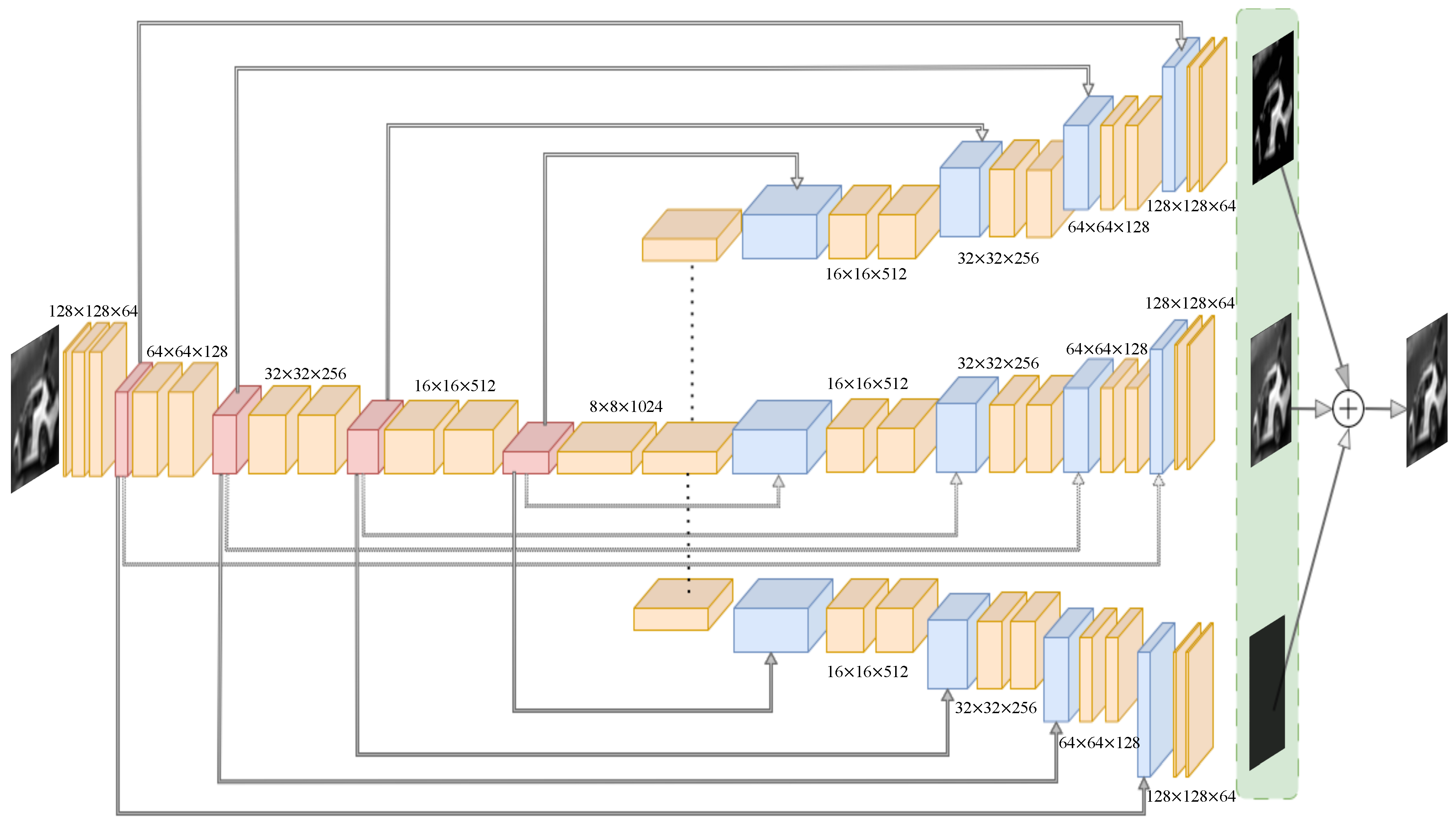
The methodology is based on an autoencoder architecture that uses images as input and is specifically designed to decompose the input data into three distinct layers: a smooth layer capturing coarse structural information, a detail layer representing fine-grained features, and a residual layer containing the remaining, often irrelevant, information as shown in Figure 1. This layer-wise decomposition aligns naturally with the autoencoder’s core objective of reconstructing the input from a compact and structured representation. Unlike standard CNNs, which are typically optimized for classification and lack explicit reconstruction mechanisms, or Transformers, which are computationally intensive and less suited for localized spatial decomposition, the autoencoder enables interpretable, additive reconstruction with dedicated branches for each type of structural component. This makes it a particularly suitable choice for our goal of semantically meaningful image separation and reconstruction.

The model first applies convolutional operations to compress the input and after it splits into three branches responsible for reconstructing each of the target layers. To ensure that these layers represent the different aspects of the input data in a meaningful way, specific variational loss functions are applied. These losses enforce the separation of information across layers while preserving the overall fidelity of the reconstruction. The sum of these three outputs is expected to closely approximate the original input, allowing for effective unsupervised decomposition without the need for labeled data. This approach enables the generation of multi-scale representations even from single-channel images, potentially increasing the amount of usable information for downstream machine learning tasks.

2.2. Loss Functions

To guide the network branches to learn distinct yet complementary feature representations, we select loss functions grounded in well-established theory and practice from image processing and deep learning. Because of its simplicity and effectiveness in penalizing overall reconstruction error, as described in the foundational deep learning literature [44], researchers widely adopt the pixel-wise Mean Squared Error (MSE) loss of image reconstruction tasks. To encourage spatial smoothness in the smooth layer and reduce high-frequency noise, we employ a squared gradient penalty that approximates the Total Variation (TV) regularization principle, which has proven effective for noise removal while preserving edges in images [45]. Conversely, the detail layer directly uses the L1 norm of the gradient to impose a first-order TV loss, thus preserving important edges and fine structures through sharp transitions [46]. These complementary norms balance smoothness and edge preservation. Lastly, residual layer loss uses a logarithmic penalty that controls the scale of activations robustly, promoting sparsity and suppressing unstructured noise components. Together, this set of loss functions enables the multi-branch auto-encoder to disentangle smooth, detailed, and residual features effectively.

$$Loss\left(\widehat{f}\right)=MSE+{\mathcal{L}}_{\mathrm{smooth}}+{\mathcal{L}}_{\mathrm{detail}}+{\mathcal{L}}_{\mathrm{residual}}$$

(1)

This formulation includes a pixel-wise mean squared error (MSE) between the reconstructed image and the ground truth, along with three specialized regularization terms for smooth, detail, and residual layers, respectively, in the corresponding decoder branches.

The general form of the loss is expanded as follows:

$$Loss\left(\widehat{f}\right)=\sum _{i,j}{(\widehat{f_{i,j}}-f_{i,j})}^2+{\lambda }_1\sum _{i,j}{\left(\nabla f_{i,j}^{\left(1\right)}\right)}^2+{\lambda }_2\sum _{i,j}\left|\nabla f_{i,j}^{\left(2\right)}\right|+{\lambda }_3\sum _{i,j}log(1+f_{i,j}^{\left(3\right)})$$

(2)

Here, $\widehat{f}$ is the reconstructed image composed of the three branches $f^{\left(1\right)}$, $f^{\left(2\right)}$, and $f^{\left(3\right)}$, which correspond to the smooth, detail, and residual layers, respectively. The first term penalizes reconstruction errors. The second term enforces spatial smoothness using the squared gradient magnitude of the smooth layer $f^{\left(1\right)}$. The third term uses the $L_1$ norm of the gradient to preserve fine structures and edges in the detail layer $f^{\left(2\right)}$. The final term encourages sparsity in the residual branch $f^{\left(3\right)}$ to separate noise and unstructured information.

We begin by defining the continuous form of the smoothness loss based on the squared 2D spatial gradient:

$$\begin{array}{cc}\hfill Loss(f^{\left(1\right)},f^{\left(2\right)},f^{\left(3\right)})& =\sum _{i,j}{\left((f_{i,j}^{\left(1\right)}+f_{i,j}^{\left(2\right)}+f_{i,j}^{\left(3\right)})-f_{i,j}\right)}^2\hfill \\ \hfill & +{\lambda }_1\sum _{i,j}\left[{\left({\displaystyle \frac{\partial f_{i,j}^{\left(1\right)}}{\partial x}}\right)}^2+{\left({\displaystyle \frac{\partial f_{i,j}^{\left(1\right)}}{\partial y}}\right)}^2\right]\hfill \\ \hfill & +{\lambda }_2\sum _{i,j}\left[\left|{\displaystyle \frac{\partial f_{i,j}^{\left(2\right)}}{\partial x}}\right|+\left|{\displaystyle \frac{\partial f_{i,j}^{\left(2\right)}}{\partial y}}\right|\right]\hfill \\ \hfill & +{\lambda }_3\sum _{i,j}log(1+f_{i,j}^{\left(3\right)})\hfill \end{array}$$

(3)

To encourage spatial coherence in the output feature maps, we introduce smooth layer loss, which penalizes sharp variations between neighboring activations. This regularization is particularly beneficial in tasks such as image synthesis, segmentation, or depth estimation, where the output is expected to vary smoothly over space.

In Equation (3), $f_{i,j}^{\left(1\right)}$ represents the activation at spatial location $(i,j)$ on a given feature map, and the terms ${\displaystyle \frac{\partial f_{i,j}^{\left(1\right)}}{\partial x}}$ and ${\displaystyle \frac{\partial f_{i,j}^{\left(1\right)}}{\partial y}}$ denote the partial derivatives of the activation values in the horizontal and vertical directions, respectively. This expression corresponds to the squared norm of the 2D gradient vector, which serves to penalize large changes in the feature map between adjacent positions.

In practice, neural networks operate on discrete grid-based data, so we approximate the continuous partial derivatives using forward finite differences:

$${\displaystyle \frac{\partial f_{i,j}^{\left(1\right)}}{\partial x}}\approx f_{i+1,j}^{\left(1\right)}-f_{i,j}^{\left(1\right)},{\displaystyle \frac{\partial f_{i,j}^{\left(1\right)}}{\partial y}}\approx f_{i,j+1}^{\left(1\right)}-f_{i,j}^{\left(1\right)}$$

(4)

These approximations in Equation (4) estimate the local change in activation values by computing the difference between a pixel and its immediate neighbor in the corresponding direction. Forward difference usage is computationally efficient and is widely used in discrete image processing.

Substituting these approximations into Equation (2), we obtain the discretized version of the smooth layer loss in Equation (5).

$${\mathcal{L}}_{\mathrm{smooth}}\approx {\lambda }_1\sum _{i,j}\left[{\left(f_{i+1,j}^{\left(1\right)}-f_{i,j}^{\left(1\right)}\right)}^2+{\left(f_{i,j+1}^{\left(1\right)}-f_{i,j}^{\left(1\right)}\right)}^2\right]$$

(5)

This formulation penalizes high-frequency components in the spatial structure of the feature map by minimizing the squared differences between adjacent pixels. As a result, it promotes locally smooth outputs and reduces visual artifacts such as noise. The hyperparameter ${\lambda }_1$ controls the relative strength of this regularization term in the total loss function.

The entire loss term is differentiable and compatible with automatic differentiation frameworks. In the implementation, it can be computed efficiently using convolutional filters or element-wise operations on tensor slices.

In addition to encouraging global smoothness, it is often desirable to preserve important local details such as edges and texture boundaries. To this end, we introduce a detail layer loss, which penalizes the absolute magnitude of the spatial gradients. This formulation aligns with the concept of total variation (TV) regularization, a well-known technique in signal processing and computer vision.

In Equation (3), the loss of detail layer computes the total variation by summing the absolute values of the first-order derivatives across both spatial directions. It encourages the solution to be smooth in part while allowing for sudden changes when necessary. As in the previous section, we approximate the partial derivatives on a discrete grid using forward finite differences in Equation (6).

$${\displaystyle \frac{\partial f_{i,j}^{\left(2\right)}}{\partial x}}\approx f_{i+1,j}^{\left(2\right)}-f_{i,j}^{\left(2\right)},{\displaystyle \frac{\partial f_{i,j}^{\left(2\right)}}{\partial y}}\approx f_{i,j+1}^{\left(2\right)}-f_{i,j}^{\left(2\right)}$$

(6)

Substituting these into Equation (3) yields the discretized form of the loss of detail layer in Equation (7).

$${\mathcal{L}}_{\mathrm{detail}}\approx {\lambda }_2\sum _{i,j}\left[\left|f_{i+1,j}^{\left(2\right)}-f_{i,j}^{\left(2\right)}\right|+\left|f_{i,j+1}^{\left(2\right)}-f_{i,j}^{\left(2\right)}\right|\right]$$

(7)

This discretized formulation corresponds to the first-order total variation in two dimensions. It is widely used to preserve structure while reducing minor variations and noise. The hyperparameter ${\lambda }_2$ controls the strength of the regularization. Higher values increase edge preservation and denoising at the potential cost of over-smoothing fine textures.

To further regulate the scale and dynamics of the output values, we introduce a residual layer loss based on a logarithmic penalty. This function discourages large magnitudes in the output activations while maintaining numerical stability, particularly for small values.

The residual loss is defined as:

$${\mathcal{L}}_{\mathrm{residual}}={\lambda }_3\sum _{i,j}log(1+f_{i,j}^{\left(3\right)})$$

(8)

In Equation (8), $x_{i,j}$ denotes the activation value at position $(i,j)$, and ${\lambda }_3$ is a regularization coefficient. The logarithmic function applies a sublinear penalty that is growing more slowly than linear or quadratic penalties so that it is useful when it is desirable to compress the influence of larger activation values while still penalizing them.

The use of $log(1+x_{i,j})$ ensures that the function remains well-defined for non-negative $x_{i,j}$, and avoids singularities or instability near zero. This form is related to robust cost functions used in statistics and optimization. The hyperparameter ${\lambda }_3$ controls the strength of the regularization.

2.3. Model Description

In our multi-scale feature extraction framework, we propose a novel approach that enables neural networks to distinguish between different layers of information in spatial resolutions while filtering out redundant data. This methodology aims to progressively expand the depth and capacity of the network while maintaining a consistent architectural pattern across all scales.

We begin by feeding the input data into the encoder component of our model. Within the encoder, each feature extraction block consists of convolutional layers, batch normalization, and ReLU activation functions. These blocks are designed to extract features on multiple spatial scales. As the network progresses deeper, the receptive fields of the convolutional layers expand, enabling the capture of increasingly abstract representations. The encoder part, in particular, is responsible for capturing contextual information through repeated convolutional operations and downsampling via max-pooling operations. The details of the encoding part of the model are shown in

Table 1. The details of encoder part of the model.

Layer	Type	Input Channels	Output Channels	Kernel Size	Stride	Padding
Conv1	Conv2d	1	64	3 × 3	1	1
Conv2	Conv2d	64	64	3 × 3	1	1
Pool1	MaxPool2d	-	-	2 × 2	2	0
Conv3	Conv2d	64	128	3 × 3	1	1
Conv4	Conv2d	128	128	3 × 3	1	1
Pool2	MaxPool2d	-	-	2 × 2	2	0
Conv5	Conv2d	128	256	3 × 3	1	1
Conv6	Conv2d	256	256	3 × 3	1	1
Pool3	MaxPool2d	-	-	2 × 2	2	0
Conv7	Conv2d	256	512	3 × 3	1	1
Conv8	Conv2d	512	512	3 × 3	1	1
Pool4	MaxPool2d	-	-	2 × 2	2	0
Conv9	Conv2d	512	1024	3 × 3	1	1
Conv10	Conv2d	1024	1024	3 × 3	1	1

.

Following the encoding phase, as shown in

Table 2. The details of each layer for the decoder part of the model.

Layer	Type	Input Channels	Output Channels	Kernel Size	Stride	Padding
ConvTrans1	ConvTrans2d	1024	512	3 × 3	2	1
Conv1	Conv2d	512	512	3 × 3	1	1
ConvTrans2	ConvTrans2d	512	256	3 × 3	2	1
Conv2	Conv2d	256	256	3 × 3	1	1
ConvTrans3	ConvTrans2d	256	128	3 × 3	2	1
Conv3	Conv2d	128	128	3 × 3	1	1
ConvTrans4	ConvTrans2d	128	64	3 × 3	2	1
Conv4	Conv2d	61	64	3 × 3	1	1
Conv5	Conv2d	64	1	3 × 3	1	1

, the decoder component of our model, composed of expanding paths, facilitates the reconstruction of high-resolution features from the encoded representations. Skip connections are used to bridge the encoder and decoder pathways, allowing for the integration of low-level spatial information from earlier layers with high-level semantic features learned in deeper layers. Our architecture includes three symmetric expanding paths, each designed to extract and reconstruct different levels of information from the encoded data. At the end of each path, distinct loss functions are applied to guide the reconstruction process. The first path aims to recover a smooth approximation of the original data, the second emphasizes the preservation of fine details, and the third is structured to capture redundant or residual information. The fusion of these three outputs is intended to accurately reconstruct the input data, ensuring both structural coherence and representational richness.

3. Experiments

In this section, we examine the effectiveness of the proposed unsupervised multi-scale feature extraction technique, which decomposes input images into smooth, detail, and residual layers using an autoencoder architecture. We also provide comprehensive information on the datasets, tasks, and experimental setup.

3.1. Dataset and Task

To evaluate the performance of the proposed method, two tasks were conducted: a multiclass classification task on the CIFAR-10 dataset [47] and an image segmentation task on a medical CT dataset [48]. CIFAR-10, a widely recognized benchmark developed by the Canadian Institute for Advanced Research, contains 60,000 colored images with a resolution of 32 × 32 pixels, equally distributed across 10 diverse classes. All CIFAR-10 images were preprocessed by resizing to 128 × 128 pixels using bicubic interpolation, converting them to single-channel grayscale, and transforming them into tensor format. The training set was used to train the model, while the test set was reserved for performance evaluation. The diverse nature of CIFAR-10 helps expose the model to various visual patterns, improving feature learning. Although hyperspectral and RGB image datasets provide richer information, practical constraints such as computational resources and hardware limitations restricted their use in this study. Therefore, CIFAR-10 was selected as a computationally efficient dataset to demonstrate the method’s capabilities.

In addition, to demonstrate the effectiveness of the proposed method in a more complex and practical application, an image segmentation task was performed using a high-resolution medical CT dataset [49] focused on lung segmentation. This dataset consists of 267 manually segmented CT scans with a resolution of 512 × 512 pixels. Accurate lung segmentation is a critical preprocessing step in tasks such as lesion detection and disease classification. Including this dataset provides additional validation of the applicability of the proposed method in real-world medical imaging scenarios, highlighting its robustness in higher-resolution grayscale data.

3.2. Experimental Settings

The proposed method was developed using the Python 3.11.5 programming language, which offers extensive support for scientific computing and deep learning research. The PyTorch 2.0.1 deep learning library was selected for the implementation of the proposed deep learning model. The implementation was carried out in an environment equipped with an AMD Ryzen 9 7950X 16-core processor, 32 GB of RAM, and an 8 GB GeForce RTX 3080 Ti GPU. To evaluate the performance of the model, several key metrics were used, including precision, recall, F1 score, test set accuracy for the classification and confusion matrices. Together, these metrics offer a comprehensive view of the model’s classification performance.

3.3. Experimental Configurations

To evaluate the proposed method, several pre-trained network architectures that accept three-channel inputs were used. The ResNet-18 [50], ResNet-50 [51], and MobileNetV2 [52] architectures were used to analyze the impact of newly generated features on classification performance. ResNet-18 and ResNet-50 are deep residual networks designed to address the problem of vanishing gradient through residual connections, which allows the training of deep networks. ResNet-18 consists of 18 layers, while ResNet-50, with 50 layers, enables more complex feature extraction. MobileNetV2 is a lightweight architecture optimized for efficient performance on mobile and embedded devices. Using separable convolutions to reduce computational complexity while maintaining high classification accuracy.

The evaluation process began with the extraction of the residual layer from the output of the proposed method. The smooth and detailed components were then merged with the original input to form a new three-channel representation, which served as input for the ResNet-18, ResNet-50, and MobileNetV2 networks to evaluate the classification performance. In addition, a separate test was conducted using the same networks, where no pre-preprocessing was applied to the input images. Instead, a grayscale version of each image was replicated across all three channels to form the input. The details of the hyperparameters used in the training process of the proposed model are shown in

Table 3. Hyperparameter details of the proposed method.

Parameters	Values
Input Size	128 × 128
Initial Learning Rate	0.00001
Optimizer	Adam
Batch Size	16
Cost Function	MSE + ${\mathcal{L}}_{\mathrm{smooth}}+{\mathcal{L}}_{\mathrm{detail}}+{\mathcal{L}}_{\mathrm{residual}}$
${\lambda }_1$ (Smoothness Loss Weight)	1
${\lambda }_2$ (Detail Loss Weight)	4
${\lambda }_3$ (Residual Loss Weight)	3
Epoch	100

.

In our experiments, ${\lambda }_1$, ${\lambda }_2$, and ${\lambda }_3$ values for proposed loss functions were assigned fixed values to maintain consistency and ensure stable convergence during training. These values were empirically determined through preliminary experiments in a validation subset of the training data. The aim was to balance the influence of each branch so that the smooth and detail layers capture meaningful structural information while the residual layer suppresses noise or irrelevant patterns. Improper tuning of the regularization coefficients can lead to ineffective decomposition of the image features across the respective layers. In such cases, most of the image information can be gathered in a single layer, causing the other layers to become redundant or uninformative. This undermines the model’s ability to decompose the image into smooth, detailed, and residual components as intended. This parameter tuning represents a challenging aspect of the proposed method. Therefore, careful adjustment of these parameters is essential to ensure that each layer captures distinct and meaningful features, ultimately enhancing the quality of feature extraction and improving model performance.

Besides classification, the proposed method was further evaluated on an image segmentation task using a lung CT dataset. The pre-trained multibranch autoencoder model, originally trained on CIFAR-10, was used to decompose each CT image into smooth, detailed, and residual components. For this experiment, the residual layer was excluded, which is typically the source of redundant information and noise, and the original image was used in its place. These components were then combined and used as input to a U-Net [53] segmentation model. In addition, we performed an ablation study by training the segmentation network in different combinations of smooth layer, detail layer, and original image to validate the contribution of each component.

These experiments assessed the impact of the proposed method on the extractable information from the data and evaluated how these newly generated representations influence the performance of machine learning models built upon them.

3.4. Experimental Results

The performance of the proposed model was evaluated using the CIFAR-10 test dataset. To assess its effectiveness, standard classification metrics are used, including precision, recall, F1-score, accuracy, and confusion matrix. Precision and recall were calculated using Equations (10) and (11), where TP denotes true positives, TN denotes true negatives, FP denotes false positives, and FN denotes false negatives. The F1-score was calculated using Equation (12).

$$\mathrm{Accuracy}={\displaystyle \frac{\mathrm{TP}+\mathrm{TN}}{\mathrm{TP}+\mathrm{TN}+\mathrm{FP}+\mathrm{FN}}}$$

(9)

$$\mathrm{Precision}={\displaystyle \frac{\mathrm{TP}}{\mathrm{TP}+\mathrm{FP}}}$$

(10)

$$\mathrm{Recall}={\displaystyle \frac{\mathrm{TP}}{\mathrm{TP}+\mathrm{FN}}}$$

(11)

$$\mathrm{F}1=2\ast {\displaystyle \frac{\mathrm{Precision}\ast \mathrm{Recall}}{\mathrm{Precision}+\mathrm{Recall}}}$$

(12)

The outputs of the proposed method are used as inputs for the specified deep learning models and compared with the models’ performance when using grayscale images as input. Across all models, the proposed method consistently outperforms the grayscale baseline. ResNet50 achieves an accuracy of 86.32% when using the proposed method, compared to 85.45% with grayscale inputs. Similarly, ResNet18 shows an improvement from 85.43% to 86.02%, and MobileNetV2 shows the most pronounced gain, increasing from 83.02% to 85.57%. These results suggest that the proposed method provides a more informative input representation, leading to better classification performance across different architectures, as shown in

Table 4. Classification performance on CIFAR-10 test dataset.

Model	Proposed Method				Grayscale Images
	Accuracy (%)	Precision	Recall	F1-Score	Accuracy (%)	Precision	Recall	F1-Score
ResNet18	86.02	0.86	0.8602	0.86	85.43	0.8561	0.8563	0.8560
ResNet50	86.32	0.8631	0.8632	0.8629	85.45	0.8541	0.8545	0.8540
MobileNetv2	85.57	0.8567	0.8557	0.8559	83.02	0.8331	0.8302	0.8308

.

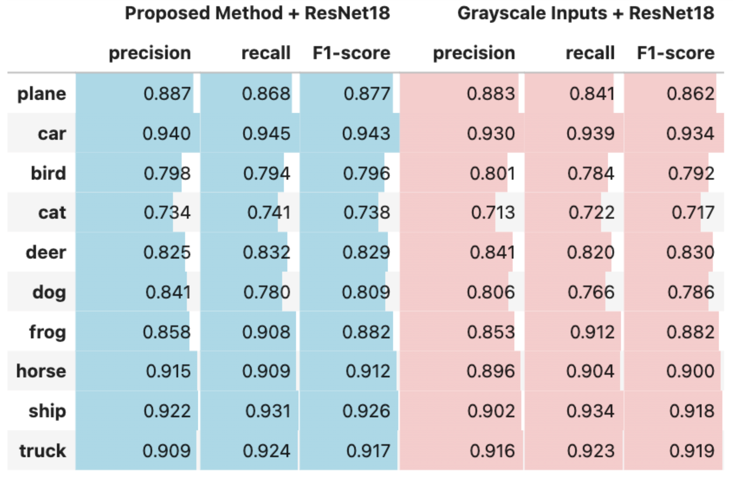
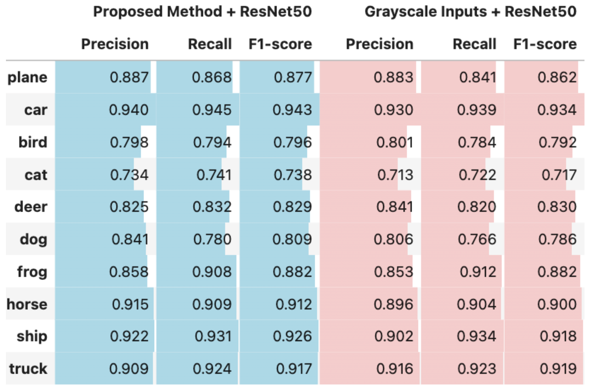
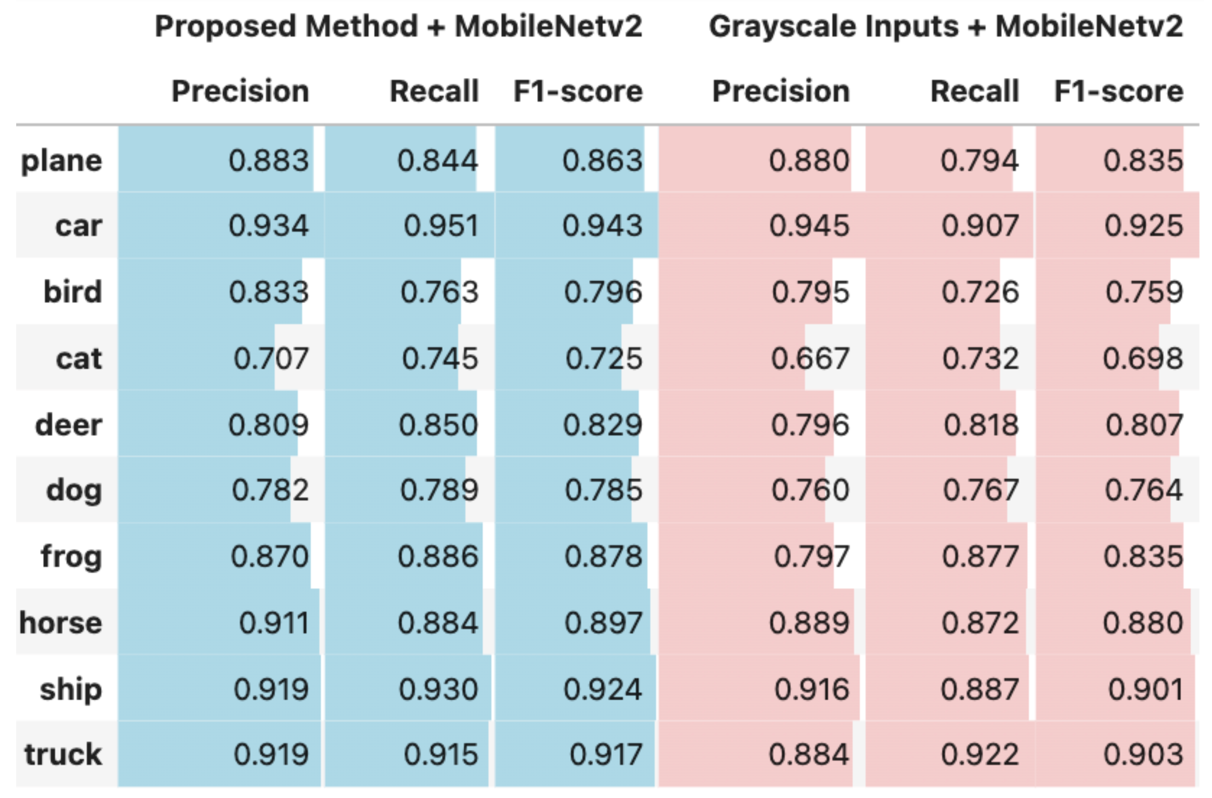
Figure 2, Figure 3 and Figure 4 present comparative analyses of precision, recall, and F1-score. These comparisons illustrate the performance differences between using the output of the proposed method as input to deep learning models and using grayscale images as input to the same models ResNet18, ResNet50, and MobileNetV2.

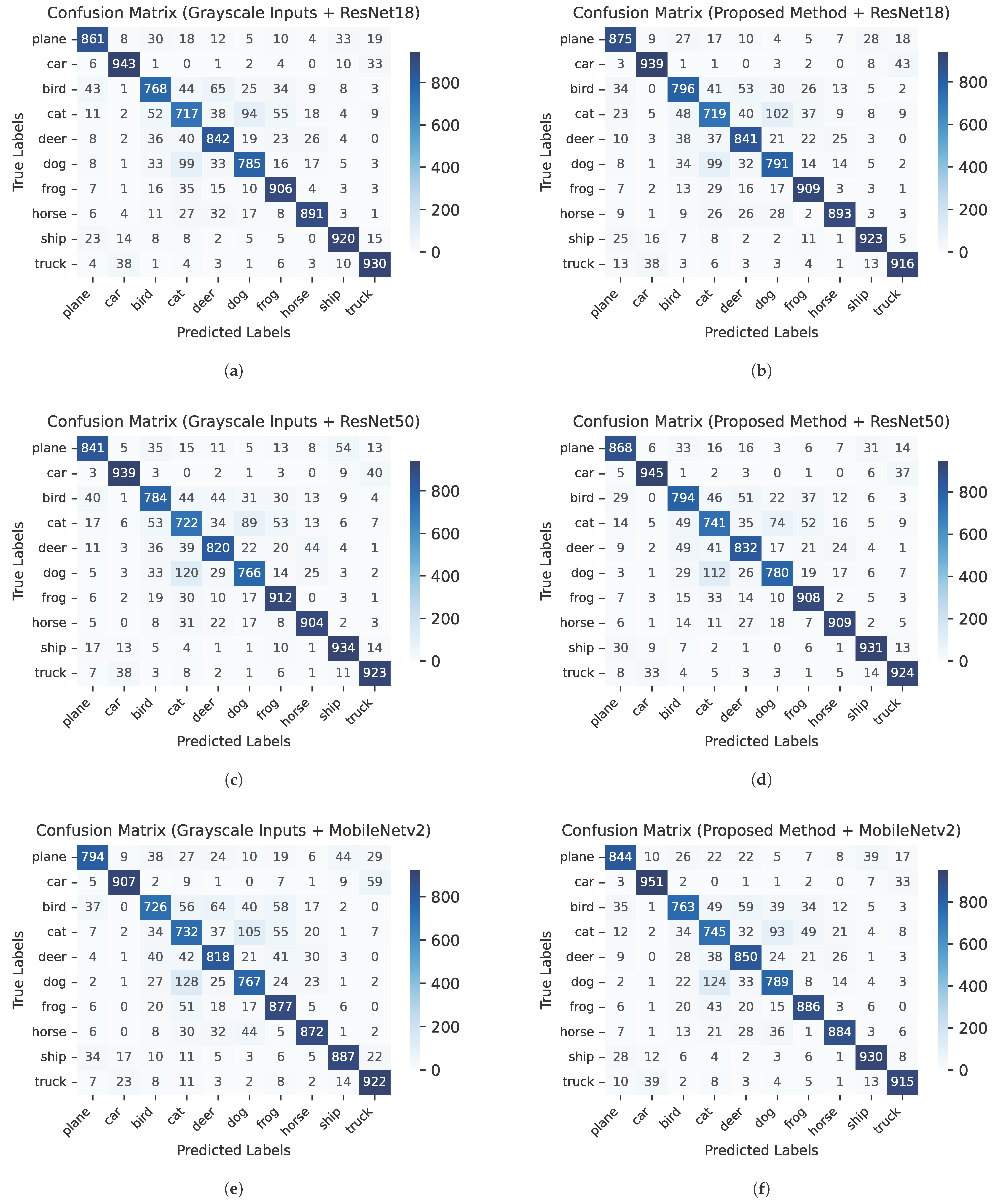
Figure 5 illustrates the confusion matrices for each experimental configuration, highlighting the impact of the proposed method compared to grayscale image inputs across three deep learning architectures: ResNet18, ResNet50, and MobileNetV2. A comparative analysis reveals that the proposed feature extraction approach consistently enhances classification performance. With ResNet18, for example, the number of correctly classified samples increased significantly in classes such as plane (from 861 to 875) and bird (from 768 to 796). Similarly, ResNet50 demonstrated improvements in the classifications of plane (841 to 868), deer (820 to 832), and cat (722 to 741). MobileNetV2 exhibited particularly more gains, with correct predictions increasing in the car (907 to 951), plane (794 to 844), deer (818 to 850), and ship (887 to 930) classes. When aggregated across all classes, the total number of correctly classified samples increased by 67 for ResNet18 (from 8683 to 8750), 69 for ResNet50 (from 8717 to 8786), and 132 for MobileNetV2 (from 8597 to 8729). These results underscore the effectiveness of the proposed representation in providing more discriminative features, thereby enhancing model performance across a variety of architectures and particularly in categories where inter-class confusion is typically higher, such as car and truck or cat and dog.

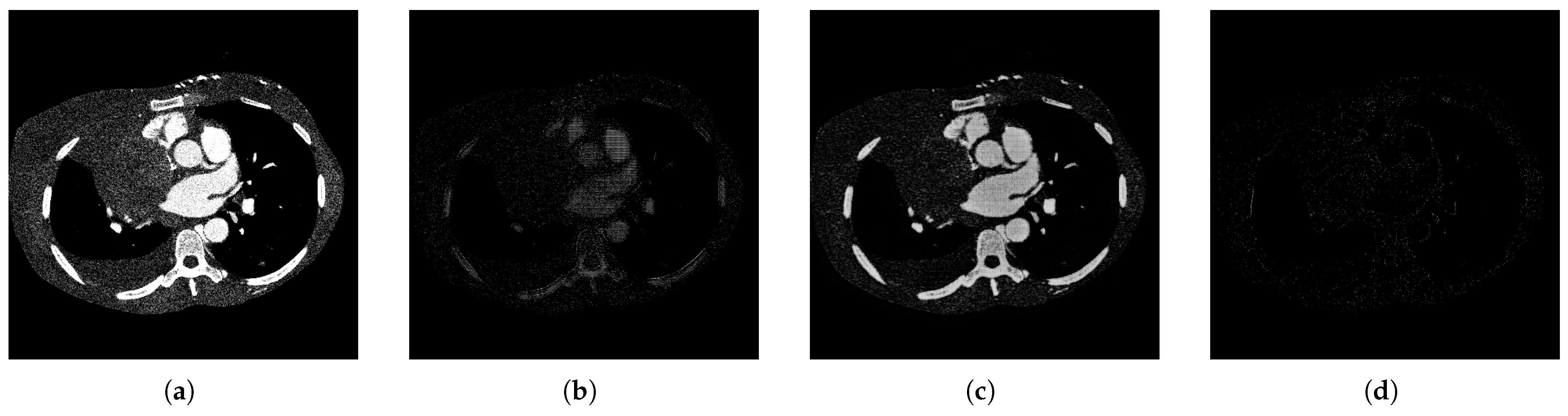
The qualitative performance of the proposed decomposition process is illustrated in Figure 6, which shows how the original image is separated into three semantically meaningful layers: a smooth layer capturing coarse structural information, a detail layer emphasizing fine textures and edges, and a residual layer isolating noise and unstructured content. As expected, the residual layer appears mostly sparse, confirming that most relevant information is effectively captured by the first two layers.

The results presented in

Table 5. Segmentation performance comparison with different input combinations.

Model	Dice Score	IoU	Pixel Accuracy
U-Net (Original Image)	0.8276	0.7646	0.9412
U-Net (Original + Smooth Layer)	0.7931	0.7417	0.9360
U-Net (Original + Detail Layer)	0.9778	0.9600	0.9897
U-Net (Original + Smooth + Detail)	0.9636	0.9355	0.9834

illustrate the impact of different input combinations on segmentation performance using the U-Net architecture. Among all configurations, the U-Net model that utilized the original image together with the detail layer achieved the highest performance across all metrics, with a Dice score of 0.9778, IoU of 0.9600, and pixel accuracy of 0.9897. This indicates that the detail component significantly enhances the model’s ability to capture fine-grained structures critical for accurate medical image segmentation.

$$\mathrm{Dice}={\displaystyle \frac{2\times |A\cap B|}{\left|A\right|+\left|B\right|}}={\displaystyle \frac{2\mathrm{TP}}{2\mathrm{TP}+\mathrm{FP}+\mathrm{FN}}}$$

(13)

$$\mathrm{IoU}={\displaystyle \frac{|A\cap B|}{|A\cup B|}}={\displaystyle \frac{\mathrm{TP}}{\mathrm{TP}+\mathrm{FP}+\mathrm{FN}}}$$

(14)

In comparison, the baseline model using only the original image achieved moderate performance (Dice: 0.8276, IoU: 0.7646, Pixel Accuracy: 0.9412), while adding only the smooth layer slightly degraded performance. Interestingly, when both the smooth and detail layers were combined with the original image, performance remained high (Dice: 0.9636), though still slightly lower than using the detail layer alone. These findings suggest that while smooth features may dilute fine details when used in isolation, they can still complement high-frequency detail features in multi-scale representations. Ultimately, the detail layer is the most influential factor in improving segmentation quality, and its integration into the input representation leads to significant gains in accuracy and robustness.

4. Discussion

The primary contribution of this study is the introduction of an unsupervised multi-scale feature extraction model inspired by scale-space theory. Rather than targeting state-of-the-art performance, the goal is to offer a modular and interpretable preprocessing technique that enriches feature representations and improves downstream task performance.

Our experiments on classification and segmentation tasks demonstrated the model’s ability to enhance both the diversity and relevance of extracted features. In segmentation, the decomposed layers—particularly the detail and smooth components—proved effective in isolating structural details and suppressing irrelevant variations.

Despite using relatively small datasets and conventional models, the architecture is inherently scalable. Its fully convolutional design allows seamless operation on various image sizes that are multiple of 16 (e.g., 512 × 512) without structural modification. This flexibility enables re-training, fine-tuning, or plug-and-play use with pre-trained weights, making the model suitable for broader applications in medical imaging, remote sensing, and other domains requiring multi-scale analysis.

5. Conclusions

In this study, we proposed an unsupervised multi-scale feature extraction mechanism capable of decomposing image content into smooth, detailed, and redundant components. The proposed approach demonstrated promising results in improving classification performance by increasing the representational capacity of the input data. Specifically, on a 10-class dataset, our method led to accuracy improvements of up to 3 percent, underscoring its potential to support and strengthen downstream tasks.

Beyond classification, we evaluated the model on an image segmentation task using 512 × 512 resolution medical images. The decomposed layers, particularly the detail component proved effective in capturing fine structures essential for accurate boundary delineation, while the smooth layer helped suppress irrelevant background information. These results highlight the model’s utility in tasks where spatial precision is critical, such as biomedical or remote sensing image analysis.

In addition to its quantitative benefits, the model offers several practical advantages: it preserves the structural integrity of the input, enriches feature representations without requiring supervision, and remains adaptable to datasets and architectures of varying complexity. Its fully convolutional design enables the straightforward deployment of inputs with compatible dimensions, enhancing its flexibility in real-world applications.

Future work will focus on assessing the model’s effectiveness across broader domains beyond classification and segmentation, including anomaly detection, image synthesis, and remote sensing. Furthermore, investigating the sensitivity and robustness of the model to different hyperparameter settings, such as regularization weights and architectural configurations will be crucial to ensure stability across varied datasets and tasks.