Cumulative Failure Rate Prediction of EDCU in Subway Vehicles Based on RF–CNN–LSTM Model

Abstract

Based on the current research status of fault prediction in rail transit reliability, this paper proposes a cumulative failure rate prediction method for key components of subway vehicles based on the RF-CNN-LSTM model. The article describes the prediction method based on cumulative failure rate data and takes the subway EDCU as an example of cumulative failure rate prediction. Three models, ARIMA, MLP, and LSTM, are introduced and compared with the RF–CNN–LSTM model by R² and adjusted R² index. The results show that the RF–CNN–LSTM model can predict the failure rate of the underground door controller well, with accuracy rates of 99.78% and 97.88%. Based on the prediction results, the cumulative failure rate of the EDCU peaks in about 10 years at 4.5% and 10.6%, respectively; the maintenance strategies can be adjusted through the actual situation of the EDCU to reduce maintenance costs and optimize maintenance plans.

1. Introduction

Subway vehicles contain many key systems and key components. The reliability of key systems and key components directly affects the travel safety of most passengers and provides an important basis for the maintenance of subway vehicles. At present, urban rail transit metro vehicle failure prediction research mainly focuses on subsystems and passenger flow, while in the actual maintenance process, the failure rate of key components is an important indicator of vehicle maintenance. At the same time, there will be excessive maintenance and under repair in maintenance. Therefore, it is very important to carry out a prediction study on the failure rate of the key components of metro vehicles, which can provide data to support the safety of metro vehicle maintenance as well as the accuracy of the maintenance plan, thus reducing maintenance cost.

Su Hang et al. [1] established a reliable BP neural network by choosing appropriate network parameters and realized a subway signal equipment fault prediction system through the MATLAB v7.0 visual graphical interface GUI; based on the prediction of the BP neural network, Wei Qianzhou et al. [2] combined the particle swarm algorithm with the BP neural network to form a new prediction model, and predicted the failure of subway shield doors; Xiang Ling et al. [3], since the particle swarm algorithm and bp neural network were prone to algorithmic instability problems, proposed combining the ant colony algorithm with the BP neural network, constructed a new model of PSD residual life prediction, and effectively proved the stability and accuracy of the proposed GA–BP algorithm through experimental examples; Li Bowen et al. [4] proposed an improved BP neural network algorithm for predicting faults in rail circuits with a dragonfly algorithm to optimize and improve the weights and thresholds of the initial BP neural network, used track voltage data collected by the electric workshop to train the improved BP neural network, and predicted and analyzed the rail out 1 and rail out 2 voltage values of the track circuit to obtain the probability of the occurrence of the red band and the trend of the track circuit; Burak Kizilöz et al. [5] proposed a serial (STDM) and artificial neural network (ANN) combination model for the daily failure rate of the water distribution network, which can improve prediction accuracy; Qingfu Li et al. [6] proposed a back-propagation neural network based on the optimization of genetic algorithms to simulate and predict pipeline failures, so as to improve the accuracy of pipeline failure prediction; Zhiru Wang et al. [7] applied the theory of task-driven behaviors and the theory of the system to reveal the general framework of MRTS applied the task-driven behavioral theory and system theory to reveal a general framework for escalator accident mechanisms and used Lasso-Logistic Regression (LLR) for escalator damage prediction; Wang Hao [8] proposed a two-stage train delay prediction method based on data smoothing and multi-model fusion, which is effective in predicting train delays; Wang Lei et al. [9] built a model combining analytical ripple and GM(2,1) for online aging monitoring and life prediction of electrolytic capacitors for power supply in urban rail transit systems; Dong Xianguang et al. [10] built a Weibull distribution combined with ratio–ratio to construct a prediction model with Bayesian assurance of data accuracy to predict the number of meter faults; Du Ying et al. [11] came up with a novel model based on the Bayesian neural network (BNN) for predicting the number of distribution faults for predicting weather-related failures in distribution systems caused by wind, rain and lightning, through which confidence intervals for the prediction results can be obtained, providing sufficient information to guide the risk management of utility companies; Yingjie Tian et al. [12,13] proposed a Bayesian and hyperellipsoid-based brake system reliability analysis, by which the accuracy of brake system reliability analysis can be improved; Rodney Kizito et al. [14] proposed an LSTM model based on the PdM background for predicting equipment failures, estimating the probability of failure and the RUL, and compared it with the random forest model to obtain a method that performs relatively well in fault classification and outperforms RF in RUL prediction.

There are still some problems with the above fault prediction methods; for example, the problems with machine learning methods are mainly the high cost of prediction and the large amount of data needed for support. The BP neural network and Bayesian method has the problem of high requirements for initial data and parameter selection and is prone to the problem of gradient explosion. The LSTM method can deal with the problem of gradient explosion, but it has limitations for the processing of long sequence data. In the subway vehicle overhaul process, failure rate [15] is an important indicator in the reliability assessment, which cannot be ignored, and is often combined with time series in the prediction process. Time series [16] analysis is a statistical method used to analyze and process dynamic data for predicting future trends by analyzing and mining the previous development of specific data, which, after being combined with the failure rate, will lead to a relatively small amount of data and relatively short time sequences, making it difficult to make accurate predictions using the above model.

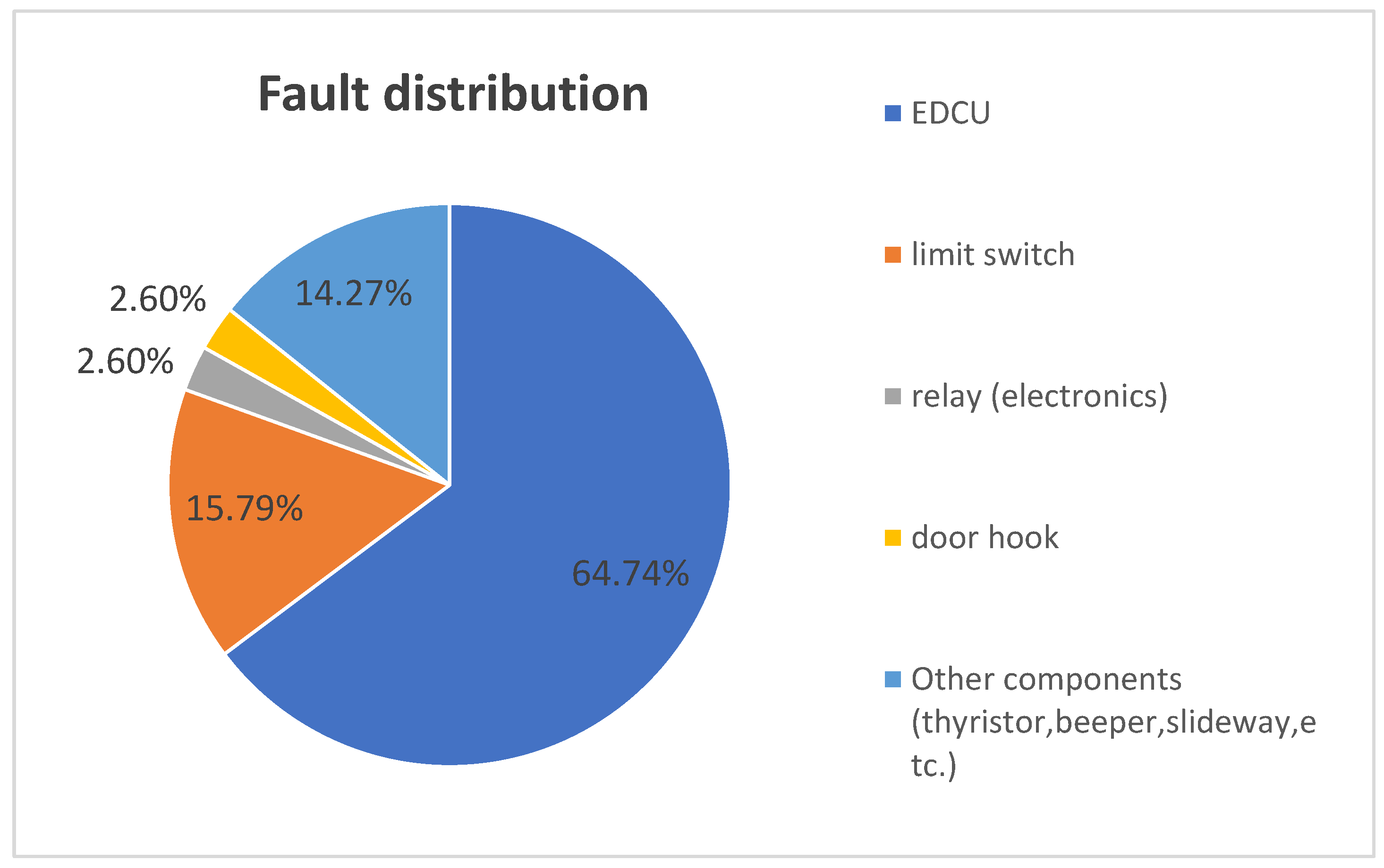
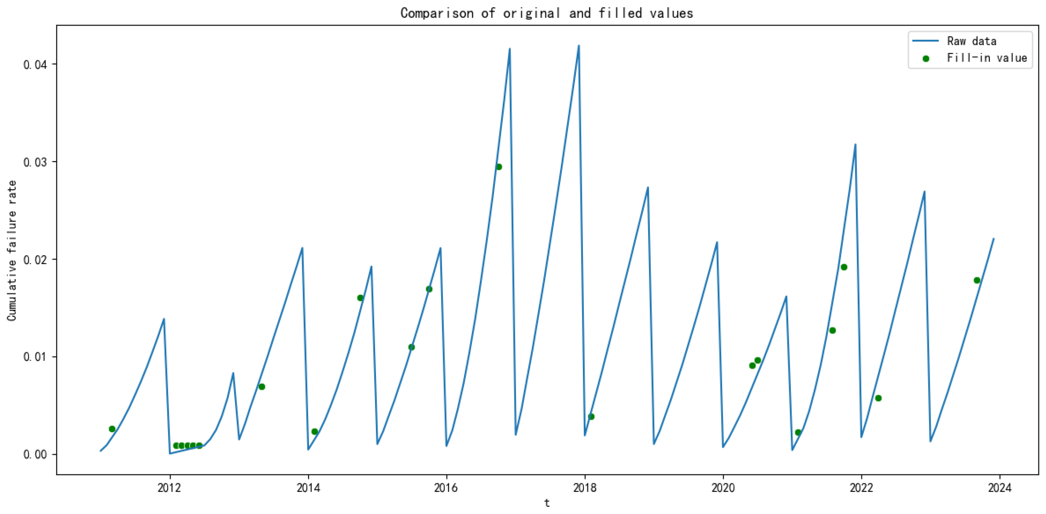
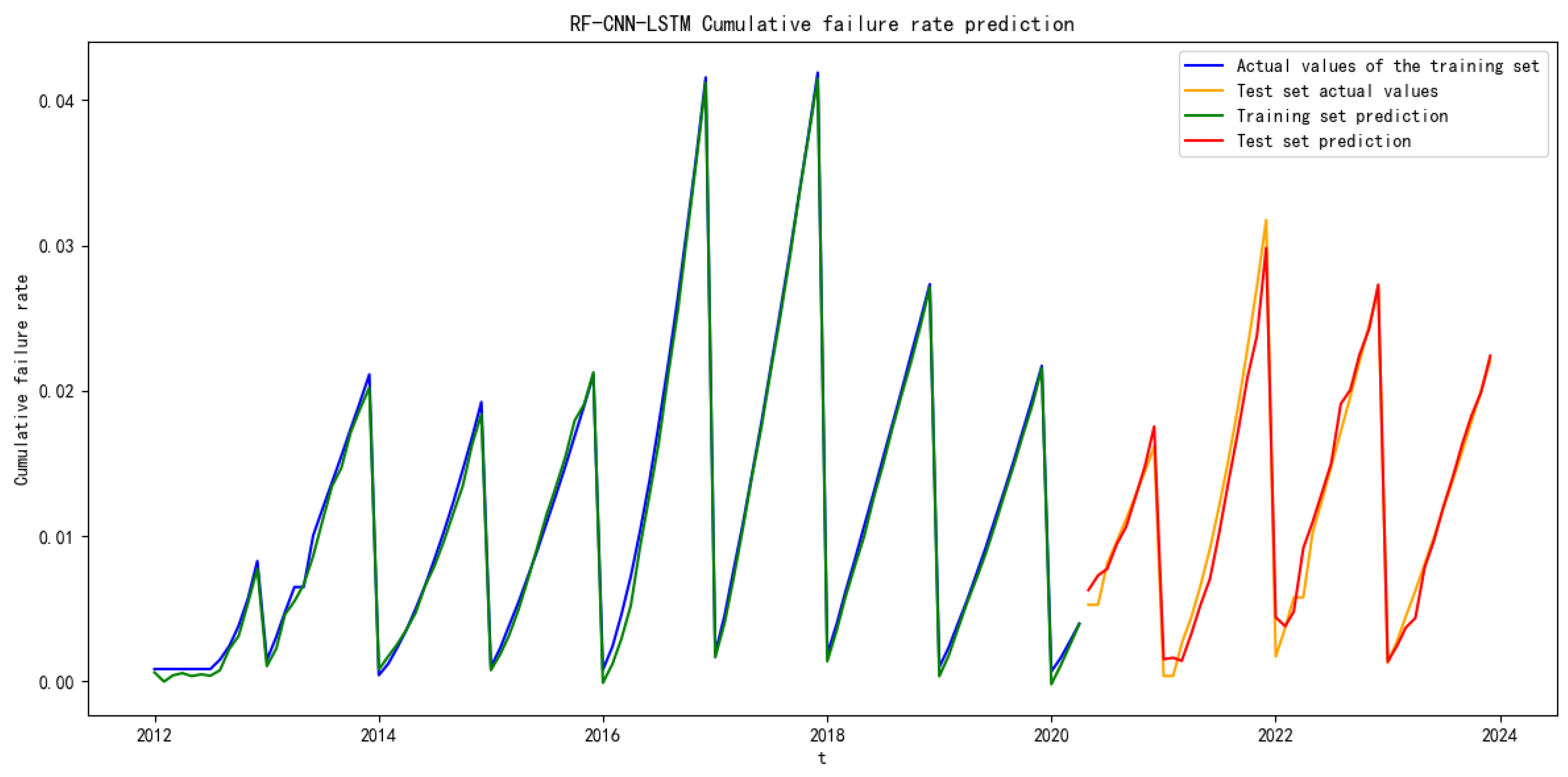
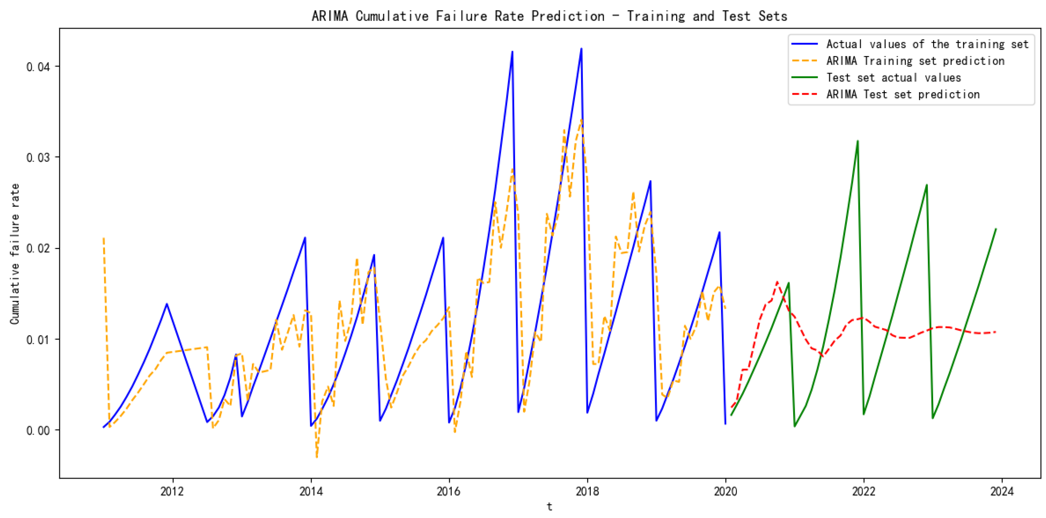
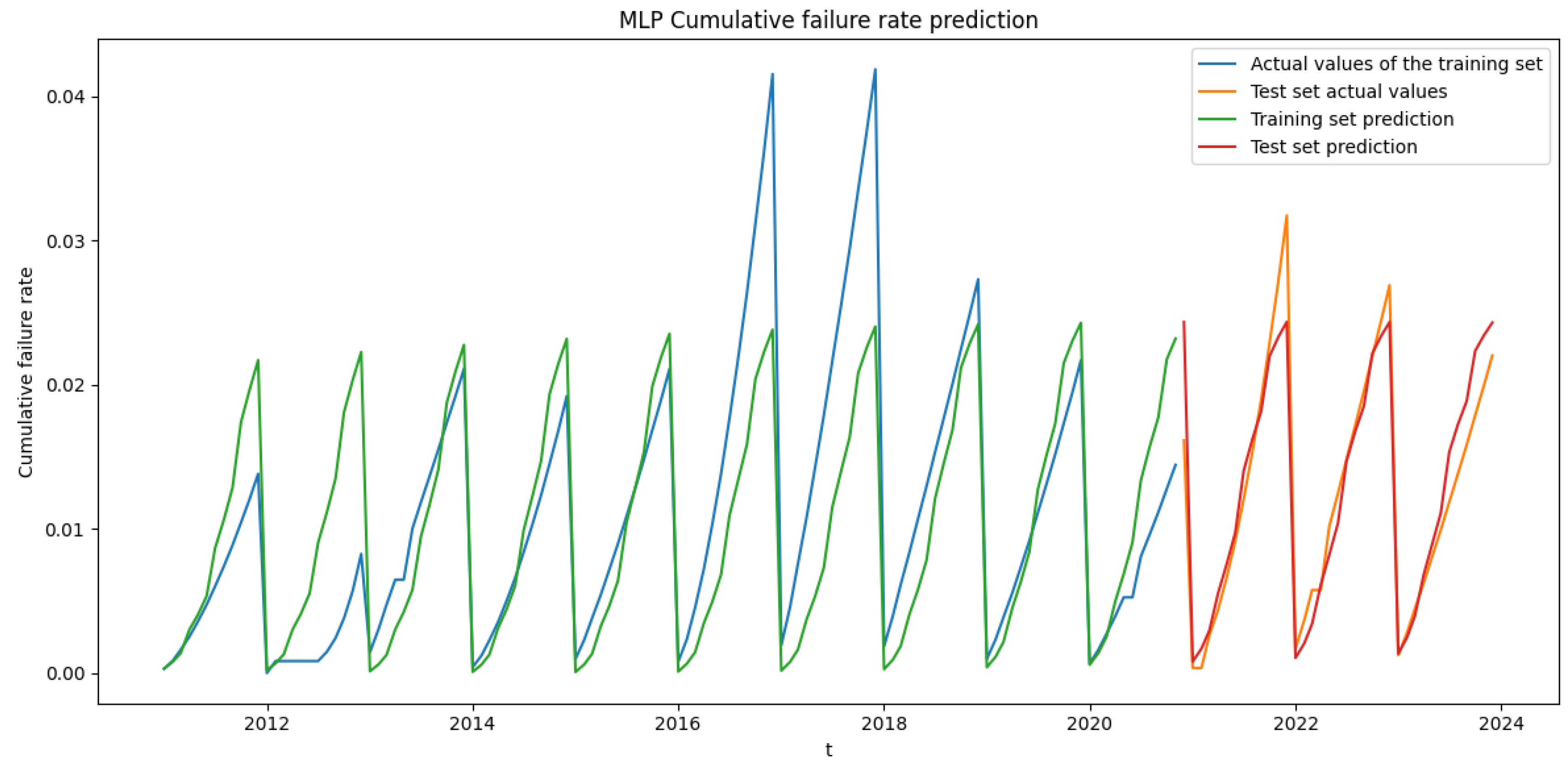
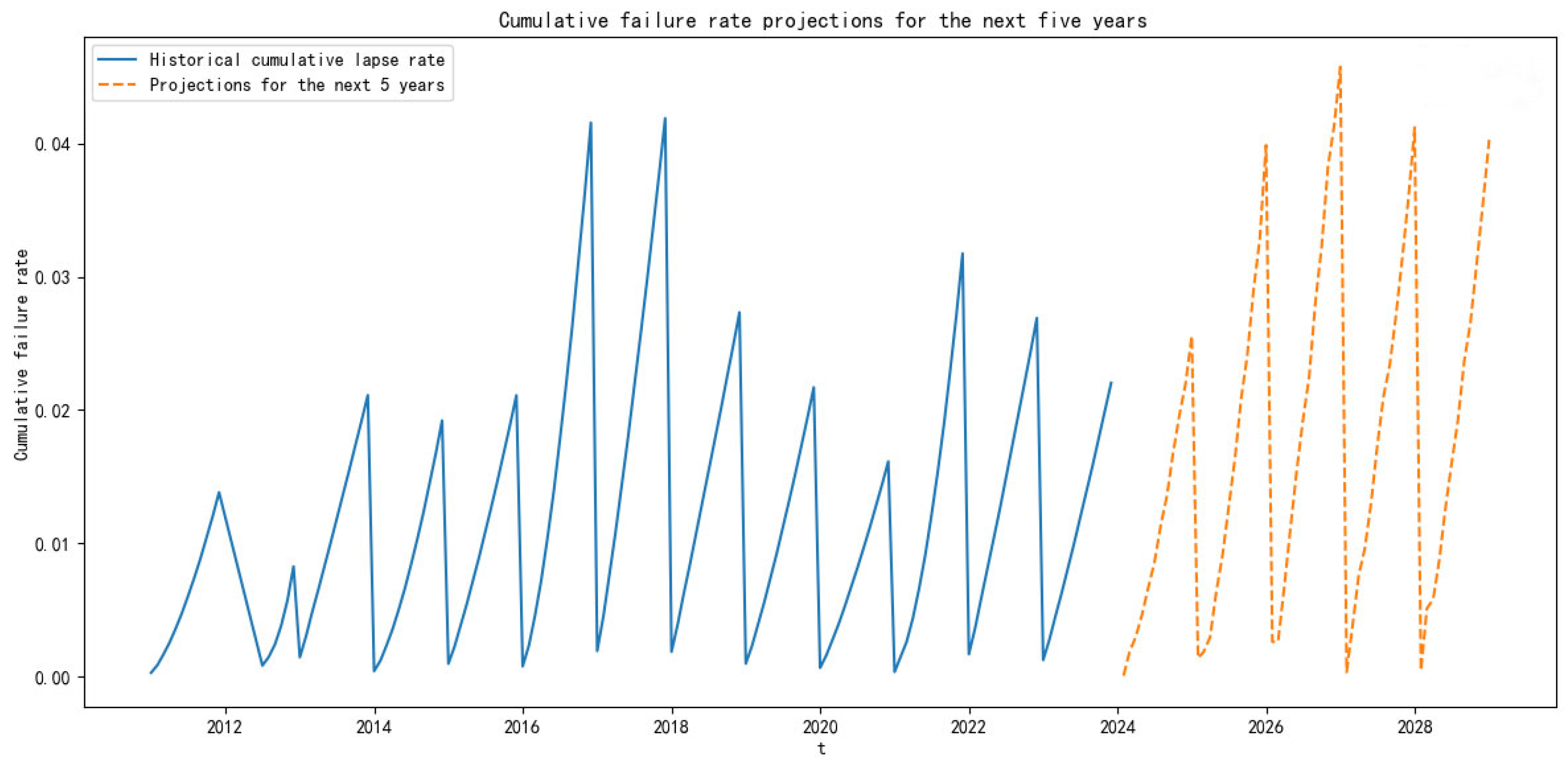
This paper proposes a combination model based on Random Forest (RF), Convolutional Neural Networks (CNN), and Long Short-Term Memory (LSTM) to predict the failure rate of the key components of subway vehicles. Based on the actual subway failure rate data, Random Forest is applied to check for missing values in the data to ensure the quality of the prediction data, then CNN is used to extract the data features, and finally LSTM is used to predict the failure rate of key subway components. The ARIMA model, multilayer perceptron neural network model, LSTM model and the proposed RF–CNN–LSTM model are compared, and the R-squared accuracy and adjusted R-squared accuracy are introduced to evaluate the model’s prediction accuracy. Taking the door controller of the door system, a key component of the subway, as an example, the RF–CNN–LSTM model is used to predict failure rate and provide support for the preventive maintenance of EDCUs.

2. Basic Theory

This paper will use the RF–CNN–LSTM model to predict the failure rate of the subway door system EDCU. In the process of subway vehicle operation and maintenance, there may be a situation where maintenance time is too long due to the untimely supply of spare parts, and the failure data cannot truly reflect the changes in component reliability, which affects the prediction results. Therefore, this paper proposes to use Random Forest (RF) to check and fill in the missing values of the failure rate data and ensure the completeness of the data. CNN–LSTM combines the Convolutional Neural Network (CNN) with the Long Short-Term Memory Network (LSTM) for processing the sequence data with spatial–temporal characteristics. CNN is used to extract spatial features from the input data, and LSTM is used to capture temporal dependencies for more comprehensive understanding and prediction of sequence data. The model prediction results are finally evaluated by R-squared accuracy and adjusted R-squared accuracy. The specific process is shown in Figure 1:

2.1. Random Forest Model

Random Forest [17] is an integrated classification method. This paper defines a strategy for filling in missing values in time series data using Random Forest. It is assumed that a value in a time series (e.g., ‘cumulative failure rate’) is affected not only by its intrinsic trend, but also by the time (year, month) in which it occurs. The relationship between time and this value is learned by constructing a Random Forest regression model that uses the temporal characteristics corresponding to known values to predict this value at the point in time corresponding to the missing value.

The method uses temporal information as a predictor to estimate the value at the missing point in the time series through the powerful nonlinear fitting ability of Random Forest and improves the reasonableness of the filled value through simple constraints. It captures the complex patterns that may exist in the time series better than simple linear interpolation or mean interpolation.

2.2. Introduction to CNN Principles

CNN [18] is a representative deep learning network that is usually used in fields such as image recognition for processing two-dimensional signals, and its central role is to extract local features from data automatically. It is especially good at processing data with a grid structure. For time series data, CNNs can extract local patterns or trends in time through convolution operations.

2.2.1. Normalization and Training Test Splitting

Before applying CNN for feature extraction, the data needs to be normalized to the interval [−1, 1] with the formula:

$$X_{norm}={\displaystyle \frac{X-X_{\min }}{X_{\max }-X_{\min }}}\times (b-a)+a$$

(1)

where a = −1, b = 1, and X_min and X_max are the minimum and maximum values of the data, respectively.

After that the data is split into a training set and a test set.

2.2.2. CNN Section

The CNN model in this paper mainly extracts the local features of the data and reduces data dimensionality through multi-layer convolution and pooling.

Convolutional Layers

The convolution operation is performed by multiplying each element of the convolution kernel with the corresponding region of the input data and then summing up these products to obtain the value of the corresponding position on the output feature map. The convolution operation can be visualized as the kernel sliding over the input data and performing a weighted sum operation at each position to generate a pixel value for the output feature map. This process is repeated over the entire input data until all positions are covered, ultimately generating the complete output feature map. The formula is as follows:

$$(W\ast X)[i,j]=m\sum n\sum W[m,n]\cdot X[i+m,j+n]$$

(2)

where W is the convolution kernel, X is the input data, (W∗X)[i, j] denotes the pixel value at position (i, j) on the output feature map (i.e., the result of the convolution operation), W[m, n] denotes the weight of the convolution kernel W at position (m, n), X[i + m, j + n] denotes the pixel value of the input data X at position (i + m, j + n), m and n are the indexes of the convolution kernel throughout all positions of the convolution kernel, and i and j are the indexes of the output feature map, indicating the output position currently being calculated.

After each convolutional layer, an activation function is also introduced to provide nonlinear features to the data. The formula is as follows:

$$f(x)=max(0,x)$$

(3)

where x denotes the input value of the activation function, usually the sum of the weighted input and bias of a neuron.

Pooling Layer

MaxPooling is a downsampling technique used to reduce the size of the feature map while retaining the most important features. It mainly consists of three parts: dividing the region, taking the maximum value, and generating a new matrix. Dividing the region is to divide the input matrix X into multiple non-overlapping regions (pooling windows) of pool size; taking the maximum value is to take the maximum value of all the elements of each pooling window as the pooled value; generating a new matrix is to combine the maximum values of all the pooling windows into a new matrix, i.e., the pooled matrix, which is the matrix after pooling. The formula is as follows:

$$MaxPool(X)[i,j]=m,n\in poolsizemaxX[i+m,j+n]$$

(4)

where MaxPool(X)[i, j] denotes the value of the element located at position (i, j) after applying the maximum pooling operation on the input matrix X, X denotes the input matrix that usually denotes the feature or activation maps, i and j are the rows and columns indexes of the matrix after pooling; and m and n are the row and column offsets within the pooling window.

By pooling the data, the feature dimensions can be reduced, reducing the amount of computation and the number of parameters while retaining important features and increasing the model generalization capability.

2.3. Introduction to LSTM Principles

LSTM is a time [19] recursive neural network with the ability to process and predict key information in a time series, which can avoid the problems of gradient vanishing and gradient explosion and thus, capture long-term dependencies more efficiently. The LSTM cell consists of five parts: input gate, forgetting gate, output gate, cell state, and hidden state. The details are as follows:

2.3.1. LSTM Section

Input gate: determines how much of the current input is written to the cell state. The formula is as follows:

$$i_t=\sigma (W_i\cdot [h_{\mathrm{t}-1},x_t]+b_i)$$

(5)

where i_t denotes the input gate vector at the moment t, which controls the amount of information in the new input; σ denotes the sigmoid activation function, which compresses the value between 0 and 1; W_i denotes the weight matrix of the input gate; h_t−1 denotes the hidden state vector at the moment t − 1; x_t denotes the input vector at the moment t; and b_i denotes the deviation of the input gate vector.

Forgetting gate: based on the current input and the previous hidden state, it is decided which information in the cell state needs to be forgotten. The formula is as follows:

$$f_t=\sigma (W_f\cdot [h_{t-1},x_t]+b_f)$$

(6)

where f_t denotes the forgetting gate vector at the moment t, which controls the degree of retention of past information; W_f denotes the weight matrix of the forgetting gate; and b_f denotes the bias vector of the forgetting gate.

Cell state: Divided into candidate cell state and cell update state, the candidate cell state provides possible new information for cell state updating, while the cell update state is responsible for storing and transmitting long-term dependent information. The formula is as follows:

$${\tilde{C}}_t=tanh(W_C\cdot [h_{t-1},x_t]+b_C)$$

(7)

$$C_t=f_t\cdot C_{t-1}+i_t\cdot {\tilde{C}}_t$$

(8)

where ${\tilde{C}}_t$ denotes the candidate cell state vector at the moment t for updating the cell state, tanh denotes the hyperbolic tangent activation function that compresses the value between −1 and 1, W_C denotes the weight matrix of the cell state, b_C denotes the bias vector of the cell state, C_t denotes the cell state vector at the moment t that stores the long-term information, and C_t−1 denotes the moment t − 1 of the cell state vector.

Output gate: determines which parts of the cell state are output. The formula is as follows:

$$o_t=\sigma (W_o\cdot [h_{t-1},x_t]+b_o)$$

(9)

$$h_t=o_t\cdot tanh(C_t)$$

(10)

where o_t denotes the output gate vector at the moment t, which controls the amount of output information; W_o denotes the weight matrix of the output gate; b_o denotes the bias vector of the output gate; and h_t denotes the hidden state vector at the moment t, which is also the output of the LSTM unit.

Fully Connected Layer: the LSTM outputs are converted to predictions through the fully connected layer. The formula is as follows:

$$y=Wx+b$$

(11)

where W is the weight matrix, x is the input, and b is the bias.

2.3.2. Optimization Algorithms and Inverse Normalization

After setting up the model parameters, the model needs to be trained, and, at this time, the model parameters need to be updated by an optimization algorithm. This paper chooses to apply Adam as the optimization algorithm so that the learning rate in the model is adaptively adjusted according to the historical gradient of the parameters. After, the prediction data becomes back-normalized output.

Adam Optimization Algorithm

Adam Optimizer is an optimization algorithm with an adaptive learning rate that combines the advantages of the RMSprop and Momentum methods. Adam Optimizer maintains a learning rate for each parameter, which is adaptively adjusted according to the historical gradient of the parameter. The main formulas of the algorithm are:

1

Gradient first-order matrix estimation

$$m_t={\beta }_1\cdot m_{t-1}+(1-{\beta }_1)\cdot g_t$$

(12)

where m_t is the first-order moment estimate of the gradient at the moment t; β₁ is the decay rate of the first-order moment, which is usually set to 0.9; g_t is the gradient at the moment t; and m_t−1 is the first-order moment estimate of the previous moment.

2

Gradient second-order matrix estimation

$$v_t={\beta }_2\cdot v_{t-1}+(1-{\beta }_2)\cdot {g_t}^2$$

(13)

where v_t is the second-order moment estimate of the gradient at the moment t; β₂ is the decay rate of the second-order moments, which is usually set to 0.999; g²_t is the square of the gradient at the moment t; and v_t−1 is the second-order moment estimate at the previous moment.

3

Deviation correction

$${\hat{\mathrm{m}}}_t={\displaystyle \frac{m_t}{1-{\mathrm{\beta }}_1^t}}$$

(14)

$${\hat{\mathrm{v}}}_t={\displaystyle \frac{v_t}{1-{\mathrm{\beta }}_2^t}}$$

(15)

where t is the current iteration step.

4

Parameter update

$${\theta }_t={\theta }_{t-1}-\eta \cdot {\displaystyle \frac{m_t}{\sqrt{{\widehat{v}}_t}+\epsilon }}$$

(16)

where θ_t is the value of the parameter at the moment t, θ_t−1 is the value of the parameter at the previous moment, η is the learning rate, and ϵ is a very small constant to prevent division by zero.

By optimizing the algorithm, convergence can be accelerated, and model performance can be improved.

Denormalization

Denormalization involves converting the normalized predicted values back to the original scale. The formula is as follows:

$$X_{original}={\displaystyle \frac{X_{norm}-a}{b-a}}\cdot (X_{max}-X_{min})+X_{min}$$

(17)

where X_norm is the normalized value, usually within a specific range; a and b are the lower and upper limits of the range used for normalization; and X_max and X_min are the maximum and minimum values in the original data, which are used to determine the normalized range.

3. Practical Application of RF–CNN–LSTM Model

The door electronic control unit is referred to as the Emergency Drive Control Unit (EDCU) [20], which is the core of the motorized passenger compartment door. The EDCU ensures that the door is accurately and timely closed and locked, realizing its basic on/off door function. In addition, the EDCU can also monitor the position of the door in real time, to ensure that any abnormal situation can be quickly responded to. Each subway door is equipped with an EDCU that is installed in the top box on the upper part of the door body. The principle of the common EDCU is shown in Figure 2.

The fault distribution of the key components of the door system is shown in Figure 3. According to the actual records of vehicle failure of a certain city in 2023, the fault for the door system failure mainly lied on the EDCU, with the EDCU failures accounting for 65.74% of door system failures. The EDCU directly affects the operation safety and service quality of vehicles, so research of the EDCU failure rate is significant for train safety.

Taking the subway vehicle EDCUs as the research object, the EDCU failure rate data is used as an example to use the RF–CNN–LSTM model for failure prediction. Since the data are confidential, the train models applied in this paper are replaced by vehicle type A. The EDCU of vehicle type A is selected for failure rate prediction. Vehicle type A was put into service in 2009 and underwent a frame overhaul in 2017–2020. This urban subway vehicle adopts the maintenance mode of planned repair, which carries out a frame overhaul every five or ten years. The basic information of vehicle type A is shown in

Table 1. Basic information of vehicle type A.

Model	A
Service (year)	2009
Overhaul Time (years)	2017–2020

.

The overall distribution of the EDCU faults conforms to the Weibull distribution [21]. And the EDCU fault rate data is obtained by using a two-parameter Weibull function to calculate the gate controller fault rate from the fault count data. The fault number data is shown in Figure 4.

3.1. Random Forest to Fill in Missing Values

The data is fed into the Random Forest model for missing value checking and filling, and the specific process is shown in Figure 5.

(1)

Characterization construction:

The year and month are extracted as features from the time index of the failure rate data.

(2)

Data segmentation:

The data is categorized into two parts, without and with missing values, which are used as training and test sets, respectively.

(3)

Model training:

A random forest regression model is trained using the training set data. In this model, year and month are the independent variables and the ‘cumulative failure rate’ is the dependent variable; the model learns a complex nonlinear mapping from time (year and month) to cumulative failure rate. The setup parameters are shown in

Table 2. Random Forest parameter settings.

Parameters	Value
n_estimators	100
random_state	42

.

From the table, n_estimators denotes the number of trees in Random Forest, while random_state is used to control the random state to ensure that the results are reproducible.

(4)

Missing value prediction:

Predicting missing values with a trained Random Forest model.

(5)

Data post-processing:

Because the lapse rate becomes progressively larger with time during the cycle, it is necessary to ensure that the predicted cumulative lapse rate is not smaller than the previous valid data value while not larger than the latter valid value, in order to comply with the non-decreasing nature of the cumulative lapse rate.

(6)

Integration of results

Fill in missing values and remove auxiliary features.

The results of data filling are shown in Figure 6.

As can be seen from the figure, 20 missing values were identified through Random Forest and filled in, which shows that Random Forest has a good filling effect on incomplete failure rate data.

3.2. CNN–LSTM Model Prediction

The data with the filled missing values is fed into the CNN–LSTM model and the parameter settings of the CNN–LSTM model used for this real data are given in

Table 3. CNN–LSTM parameter settings.

Parameters	Value
Of convolutional input	1
One layer of convulutional output	16
Two-layer convolutional input	16
Two-layer convolutional output	32
Three-layer convolutional input	32
Three-layer convulutional output	64
Convolution kernel (math.)	3
Zero fill	1
Nuclear pooling	2
LSTM hidden layer dimension	64
LSTM input layer dimension	64
Full link layer dimension	1
Loss funcion	MSELoss
Learning rate	0.001
Number of training sessions	400
Activation function	torch.relu

.

Implementation of the model prediction was conducted using the Python v3.7 64-bit software. Before the data is fed into the convolutional layer to extract features, one element of zero padding is added to each end of the input data to keep the length of the output data the same as the input. The model is set up with three convolutional layers and three pooling layers, outputting vectors through the convolutional layers into the pooling layer, and then reducing the dimensionality of the data through the pooling layer and outputting the data into the LSTM section, in which the number of the three convolutional layers of filters are, respectively, 16, 32, 64. The LSTM part contains 64 hidden layers, and the data can be passed through the LSTM to capture the dependencies of the time series and generate the final predictions, where the training set is 70% and the prediction set is 30%. The failure rate prediction results for vehicle type A are shown in Figure 7.

In the figure, the blue curve and the orange curve represent the actual values of the training set and the test set, and the green and red curve represent the predicted values of the training set and the test set. It can be seen that the cumulative failure rate of vehicle type A reached its maximum value in 2017, which is close to 4.2%.

In order to verify the accuracy of the model, the ARIMA model, multilayer perceptron neural network, and LSTM model are introduced in this paper to predict the failure rate and compare it with the RF–CNN–LSTM model.

The ARIMA model, also known as the autoregressive moving average model, is used in [22] to construct a time series model from univariate time series observations; the basic idea is to use a certain mathematical model to describe the data series of the forecasting object over time. The data can be predicted in the future after ensuring that the data is smooth via the different methods.

A multilayer perceptron (MLP) is a feed-forward artificial neural network model consisting of [23] an input layer, one or more hidden layers, and an output layer. Except for the input layer, each node is a neuron through which the MLP model can be trained to conform to the input data, thus enabling the prediction of.

Table 4. Parameter settings for each model.

(a) LSTM parameter settings
Parameters	LSTM
Training set	70%
Test set	30%
Number of hidden layers	64
(b) ARIMA parameter settings
Parameters	ARIMA
Training set	70%
Test set	30%
p,d,q	(5,1,4)
AIC	65.8937
(c) MLP parameter settings
Parameters	MLP
Training set	70%
Test set	30%
Number of hidden layers	4
Activation function of hidden layers	Hyperbolic tangent function
Number of output layer units	1
Output layer activation function	Identity
Error function	Sum of squares function

shows the parameter settings of the three models, and the prediction results are shown in Figure 8, Figure 9 and Figure 10. It can be seen that the three models were fitted to the training set and test set of the door controller data of vehicle type A, among which the LSTM model has a better fit.

3.3. Model Accuracy Verification

In this paper, the model is validated by both the mean R² accuracy and adjusted R² accuracy using the same proportion of the training set and test set. R² can illustrate the degree of explanation of the independent variables on the dependent variable, but with the increase in independent variables, R² will increase; in order to ensure that the model validates the results, this paper also introduces the adjusted R² squared precision. The formula is as follows:

$$R^2=1-{\displaystyle \frac{S{S}_{res}}{S{S}_{tot}}}$$

(18)

$$Adjusted R^2=1-\left[{\displaystyle \frac{S{S}_{res}/(n-k-1)}{S{S}_{tot}/(n-1)}}\right]$$

(19)

where SS_res is the Residual Sum of Squares (RSS), which represents the difference between the predicted and actual values of the model; SS_tot is the Total Sum of Squares (TSS), which represents the difference between the actual values and the mean; n is the number of samples; and k is the number of independent variables.

The closer the R² and adjusted R² values are to 1, the better the model fits the data. The results of the training set and test set accuracy calculations are shown in

Table 5. Calculation of training set and test set accuracy.

Training Set	ARIMA	MLP	LSTM	RF–CNN–LSTM
R2	0.5465	0.5965	0.9740	0.9978
Adjusted R2	0.5420	0.5879	0.9710	0.9965
Test set	ARIMA	MLP	LSTM	RF–CNN–LSTM
R2	0.0390	0.9311	0.8997	0.9788
Adjusted R2	0.0161	0.9291	0.8244	0.9610

.

As can be seen from Table 5, in the training set, the RF–CNN–LSTM prediction model and the LSTM prediction model have a higher fit, and the RF–CNN–LSTM prediction model R² accuracy and adjusted R² accuracy reach 0.9978 and 0.9965, which is higher than that of the LSTM prediction model, whereas the ARIMA model and MLP have poorer fit; in the testing. In the test set, the accuracy of the RF–CNN–LSTM model and MLP is higher; the R² accuracy and adjusted R² accuracy of the RF–CNN–LSTM model reaches 0.9788 and 0.9610, which is higher than that of the MLP, while the accuracy of the ARIMA model and the LSTM prediction model is lower. Therefore, compared with the three prediction models of ARIMA, MLP and LSTM, the RF–CNN–LSTM model proposed in this paper has a better prediction performance for the EDCU failure rate of subway vehicles.

4. Failure Rate Prediction

The RF–CNN–LSTM model is applied to predict the failure rate of the gate controller for the next five years with the parameters set in

Table 6. Parameterization of future projections.

Parameters	Numerical Value
Initial sequence	12 months
Number of cycles	60 times

.

Taking 12 months of data as the initial sequence in the already scaled failure rate series, we set up 60 cycles. For each cycle, a point in time prediction is made, and the prediction results are added to the dataset to form a new series; the model is used to make predictions on the new dataset to obtain new results, and the above steps are repeated to generate predictions of the cumulative failure rate for the next five years. The door controller failure rate is predicted for vehicle type A and vehicle type B. The basic information of vehicle type B is shown in

Table 7. Basic information on vehicle type B.

Model	B
Service (year)	2007
Overhaul Time (years)	2016–1019

, and the prediction results are shown in Figure 11 and Figure 12.

In Figure 11 and Figure 12, the solid blue line represents the actual data, and the dashed orange line represents the projected value of the data five years into the future.

The following information can be obtained from Figure 11 and Figure 12:

(1)

According to Figure 11, during the period 2011–2023, the door controller failure rate of vehicle type A reaches a maximum value of 4.2% in 2016–2017; the EDCU controller failure rate for the period 2024–2029 is the predicted data output from the RF–CNN–LSTM model, and it can be seen that the cumulative failure rate of the train’s EDCU reaches a maximum value of 4.5% in 2027. From Table 1, it can be seen that the vehicle type A was put into service in 2009 and underwent a major overhaul during the period 2017–2020, after which its cumulative failure rate decreased. For vehicle type A, the metro company conducts a frame overhaul of the vehicle every five or ten years, which is consistent with the change in cumulative failure rate exhibited in Figure 11, indicating that the frame overhaul schedule for vehicle type A is consistent with the pattern of the EDCU controller failure rate.

(2)

According to Figure 12, the EDCU controller failure rate of vehicle type B reached a maximum value of 10.6% in 2018. According to Table 7, vehicle type B was overhauled in 2016–2019, and the failure rate decreased after the overhaul, which is more consistent with the results in Figure 12; according to the prediction curve of the EDCU failure rate in Figure 12, it can be seen that the failure rates of the EDCU is higher after 2024, which are all around 10%, and the failure rate reaches the maximum value of 10.6% in 2028. Vehicles undergo a frame overhaul every 5 or 10 years, and the cumulative failure rate decreases after the overhaul, which is consistent with the pattern of change in the EDCU failure rate in Figure 12, but due to the service life of the EDCU in about 15 years, the failure rate of the vehicle type B EDCU is at a high level in its late life, and the frame overhaul may not be able to satisfy the high reliability needed for operation. Thus, a batch updating of the maintenance strategy can be considered.

(3)

From the actual and predicted data, it can be seen that the overall failure rate of vehicle type A is low, and although the failure rate decreases slightly after the implementation of the frame overhaul in 2017–2020 and 2027, the overall reliability does not affect the vehicle operation, and from an economic point of view, the planned repair cycle can be extended, or the maintenance mode of condition repair can be implemented according to the actual state of the EDCU. Vehicle type B was put into service in 2007. The failure rate increased significantly in 2018, and reliability was improved after the frame overhaul, but the failure rate was higher in the second half of the EDCU’s life, and so the maintenance strategy of batch renewal should be considered.

5. Conclusions

Based on the current situation of rail transportation failure rate prediction, this paper proposes an RF–CNN–LSTM prediction model and conducts a failure rate prediction study with the subway door system EDCU as an example. The article describes the RF–CNN–LSTM prediction model process and parameter settings in detail, and the failure rate prediction is carried out by taking the EDCU of a metro line in a city as an example and introduces the ARIMA model, the multilayer perceptron neural network model, and the LSTM model to compare with the new model proposed in this paper; and finally it evaluates all the models by the R² accuracy and the adjusted R² accuracy, with the results showing that the RF–CNN–LSTM model can predict the failure rate better than the other models, which is not the case. CNN–LSTM model can predict the failure of subway vehicle door controllers better; finally, the model is applied to predict the failure rate of door controllers in the next five years.

From the forecast results, the following conclusions can be drawn:

(1) In this paper, an RF–CNN–LSTM prediction model is used to conduct a failure rate prediction study of the subway vehicle EDCUs; the advantages of this method are to ensure the integrity of the data through Random Forests, to provide data support for prediction, and to combine the local feature extraction capability of CNN and the time-dependent capture capability of LSTM, which can understand the sequence data more comprehensively; at the same time, it can quickly extract the features and reduce the data dimension of LSTM processing, improve the overall model training efficiency, and be applied to sequence data with complex spatial–temporal patterns, such as a multivariate time series and sequences with periodicity and trend.

The introduction of the R² accuracy and adjusted R² accuracy were evaluated to assess the prediction accuracy of the model, and it was finally shown that the RF–CNN–LSTM model can predict the cumulative failure rate of the subway vehicle EDCU in a better way.

(2) By predicting the failure rate of vehicle type A and vehicle type B and analyzing the results, the failure rate of the EDCU of vehicle type A will reach the peak in about 10 years, which is 4.2% and 4.5%, respectively. The subway company carries out overhaul of the vehicle every five or ten years for vehicle type A, which shows that the overhaul plan of vehicle type A is in line with the failure rate of the door controller. The failure rate of vehicle type B reaches a peak of 10.6% about ten years after it is put into service, but the prediction curve shows that the failure rate of the EDCU is higher after 2024, all of which are around 10%, so the failure rate of vehicle type B’s EDCU is at a high level at the late stage of its life, and it may not be able to satisfy the high reliability demanded for operation through a frame overhaul, and thus, the batch updating of the maintenance strategy can be considered.

(3) In order to protect the safety of vehicle operation and service quality for key components, regardless of the actual state of the components, the maintenance mode of planned repair is often used. However, sometimes the failure rate of the key components is reduced, but the overall reliability does not affect the vehicle operation, so from an economic point of view, under the premise of reliability to meet the requirements, you can extend the planned repair cycle, or according to the actual state of the equipment, the implementation of the maintenance mode of state repair.

(4) The failure rate of urban rail transit electrical component parts is consistent with the Weibull distribution [21]. The method in this paper can also be used to research the failure rate prediction of other key electrical control units of the vehicle, such as traction control units and other components, which is of great significance to provide data support for the preventive maintenance of key electrical components of the metro subway system. However, since the key electrical components have a service life, there may be large changes in the cumulative failure rate when the components reach its service life, and at the same time, the service life of different components is also different. Therefore, the RF–CNN–LSTM model proposed in this paper is only applicable to components within their service life.

References

1. Su, H. The Subway Signal Device Failure Prediction Based on BP Neural Network. Ph.D. Thesis, South China University of Technology, Guangzhou, China, 2013. [Google Scholar]
2. Wei, Q.Z.; Zhang, Y. Intelligent prediction of metro screen door fault based on PSO-BP neural network. China Sci. Technol. Inf. 2017, 22, 82–84. [Google Scholar] [CrossRef]
3. Ling, X.; Liu, S.; Liu, Q.; Wei, Q.; Zhang, Y.; Shi, Z. Research on remaining service life prediction of platform screen doors system based on genetic algorithm to optimise BP neural network. Enterp. Inf. Syst. 2022, 16, 1864478. [Google Scholar] [CrossRef]
4. Li, B.W. Research on track circuit fault prediction method based on improved BP neural network. Technol. Innov. Appl. 2024, 14, 151–155. [Google Scholar]
5. Kizilöz, B. Prediction of daily failure rate using the serial triple diagram model and artificial neural network. Water Supply 2022, 22, 7040–7058. [Google Scholar] [CrossRef]
6. Li, Q.; Li, Z. Research on Failure Pressure Prediction of Water Supply Pipe Based on GA-BP Neural Network. Water 2024, 16, 2659. [Google Scholar] [CrossRef]
7. Wang, Z.; Pang, Y.; Gan, M.; Skitmore, M.; Li, F. Escalator accident mechanism analysis and injury prediction approaches in heavy capacity metro rail transit stations. Safety Saf. Sci. 2022, 154, 105850. [Google Scholar] [CrossRef]
8. Wang, H. A two-stage train delay prediction method based on data smoothing and multimodel fusion using asymmetry features in urban rail systems. Wirel. Commun. Mob. Comput. 2022, 2022, 5188105. [Google Scholar] [CrossRef]
9. Wang, L.; Diao, L.; Qiu, R.; Xu, C.; Wang, P. Service life prediction of electrolytic capacitors in urban rail transit based on analytical iteration and GM (2, 1) model. Math. Probl. Eng. 2017, 2017, 4982163. [Google Scholar] [CrossRef]
10. Dong, X.; Jing, Z.; Dai, Y.; Wang, P.; Chen, Z. Failure prediction and replacement strategies for smart electricity meters based on field failure observation. Sensors 2022, 22, 9804. [Google Scholar] [CrossRef]
11. Du, Y.; Liu, Y.; Wang, X.; Fang, J.; Sheng, G.; Jiang, X. Predicting Weather-Related Failure Risk in Distribution Systems Using Bayesian Neural Network. IEEE Trans. Smart Grid 2020, 12, 350–360. [Google Scholar] [CrossRef]
12. Chen, Y.; Wen, J.; Tian, Y.; Zheng, S.; Zhong, Q.; Chai, X. Dynamic Reliability Assessment Method for a Pantograph System Based on a Multistate T-S Fault Tree, Dynamic Bayesian. Appl. Sci. 2023, 13, 10711. [Google Scholar] [CrossRef]
13. Tian, Y.; Wen, J.; Zheng, S. Reliability Analysis of Vehicle Braking System Based on Hyperellipsoidal Dynamic Bayesian Network. Appl. Sci. 2025, 15, 1290. [Google Scholar] [CrossRef]
14. Kizito, R.; Scruggs, P.; Li, X.; Devinney, M.; Jansen, J.; Kress, R. Long short-term memory networks for facility infrastructure failure and remaining useful life prediction. IEEE Access 2021, 9, 67585–67594. [Google Scholar] [CrossRef]
15. Toscano, R.; Lyonnet, P. On-line reliability prediction via dynamic failure rate model. IEEE Trans. Reliab. 2008, 57, 452–457. [Google Scholar] [CrossRef]
16. Hu, Q.; Wang, J.; Xiong, J.; Zhang, M.; Fu, H.; Pei, J.; Wang, W. Experimental Research on Prediction of Remaining Using Life of Solar DC Centrifugal Pumps Based on ARIMA Model. Processes 2024, 12, 1857. [Google Scholar] [CrossRef]
17. Karabadji, N.E.I.; Korba, A.A.; Assi, A.; Seridi, H.; Aridhi, S.; Dhifli, W. Accuracy and diversity-aware multi-objective approach for random forest construction. Expert Syst. Appl. 2023, 225, 120138. [Google Scholar] [CrossRef]
18. Ruan, D.; Wang, J.; Yan, J.; Gühmann, C. CNN parameter design based on fault signal analysis and its application in bearing fault diagnosis. Adv. Eng. Inform. 2023, 55, 101877. [Google Scholar] [CrossRef]
19. Chen, Z.; Dai, M.; Liu, J.; Jiang, W.; Min, Y. Life prediction of IGBT module for nuclear power plant rod position indicating and rod control system based on SDAE-LSTM. Nucl. Eng. Technol. 2024, 56, 3740–3749. [Google Scholar] [CrossRef]
20. Li, Y.D. Preliminary exploration of functions and frequent faults of electronic door control unit (EDCU) in Nanjing metro vehicles. Mod. Urban Transit Mod. Urban Transit 2009, 4, 40–42. [Google Scholar] [CrossRef]
21. Hang, T.; Wen, J.; Zheng, B.S.; Xiao, J.H.; Zhou, F. Reliability analysis of the vehicle door system EDCU based on Weibull distribution. Eksploat. Niezawodn. Maint. Reliab. 2025, 27, 195257. [Google Scholar] [CrossRef]
22. Ray, S.; Lama, A.; Mishra, P.; Biswas, T.; Das, S.S.; Gurung, B. An ARIMA-LSTM model for predicting volatile agricultural price series with random forest technique. Appl. Soft Comput. 2023, 149 Pt A, 110939. [Google Scholar] [CrossRef]
23. Haghighat, F. Predicting the trend of indicators related to COVID-19 using the combined MLP-MC model. Chaos Solitons Fractals 2021, 152, 111399. [Google Scholar] [CrossRef] [PubMed]
Figure 1. Flowchart of RF–CNN–LSTM prediction model.
Applsci 15 07188 g001
Figure 2. Door controller schematic diagram.
Applsci 15 07188 g002
Figure 3. Fault distribution of the door system.
Applsci 15 07188 g003
Figure 4. Data on the number of failures for vehicle type A.
Applsci 15 07188 g004
Figure 5. Flowchart showing the process of using Random Forest to fill in missing values.
Applsci 15 07188 g005
Figure 6. Results of missing value filling.
Applsci 15 07188 g006
Figure 7. RF–CNN–LSTM cumulative failure rate prediction results.
Applsci 15 07188 g007
Figure 8. ARIMA prediction model results.
Applsci 15 07188 g008
Figure 9. Prediction results of MLP.
Applsci 15 07188 g009
Figure 10. LSTM model prediction results.
Applsci 15 07188 g010
Figure 11. Prediction of the RF–CNN–LSTM model for the failure rate of the EDCU of vehicle type A.
Applsci 15 07188 g011
Figure 12. Prediction of the RF–CNN–LSTM model for the failure rate of the EDCU of vehicle type B.
Applsci 15 07188 g012