
Hybrid Backbone-Based Deep Learning Model for Early Detection of Forest Fire Smoke


Abstract
1. Introduction
- An improved forest fire smoke image dataset consisting of smoke and smoke-like images was created to evaluate the performance of the deep learning model.
- Smoke and normal image data were processed and classified.
- Comparative results of a total of 30 object detection models, including 20 models with modified backbone structures and 10 original Yolo models, were shared.
- An optimized model for the early detection of forest fire was proposed.
- With the proposed model, pre-fire smoke images were detected more accurately and quickly, and the accuracy of smoke detection increased.
- Compared to the original Yolo model, the number of parameters of the proposed model was reduced by 19.7%, and the number of GFLOPs was reduced by 26.8%.
- The processing power was reduced by decreasing the parameter and GFLOP values, and accordingly, the processing time was reduced by 22.7%, and the model size by 19.7%.
- Model backbone development techniques were used for the network architecture, detection accuracy, and processing speed.
- We ensured that the proposed model had higher accuracy than different Yolo models.
2. Related Works
3. Material and Method
3.1. Object Detection and Deep Learning
3.2. Dataset
3.3. Algorithms
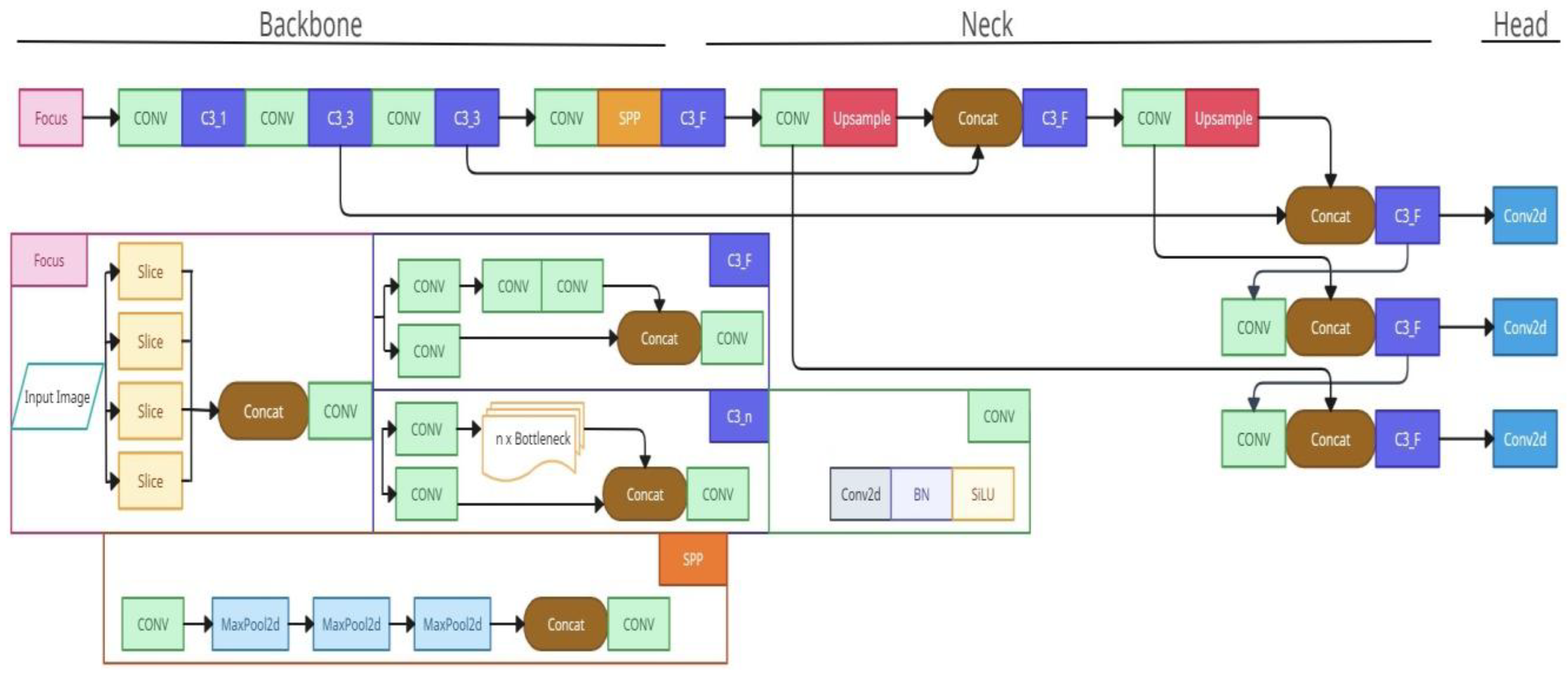
3.4. Proposed Model
3.5. Running the Models
3.6. Evaluating the Results of Object Detection Algorithms
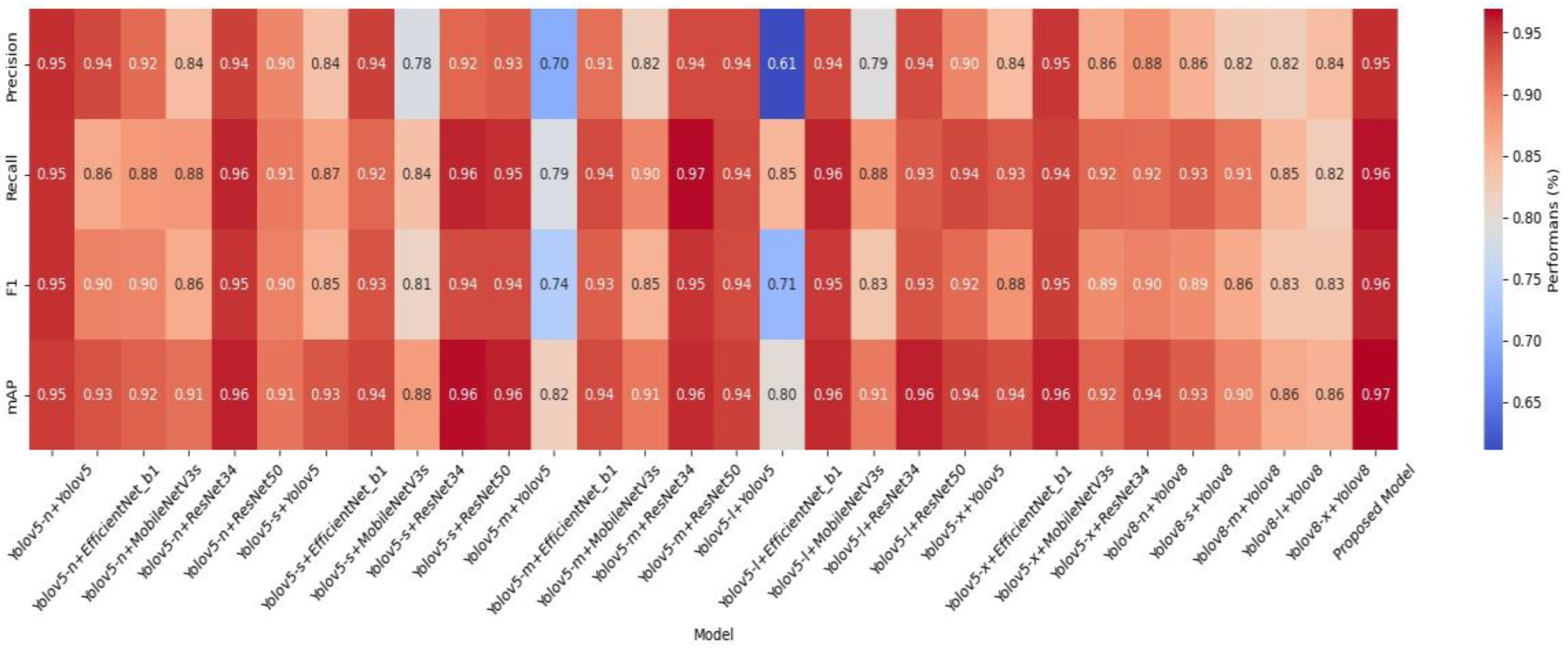
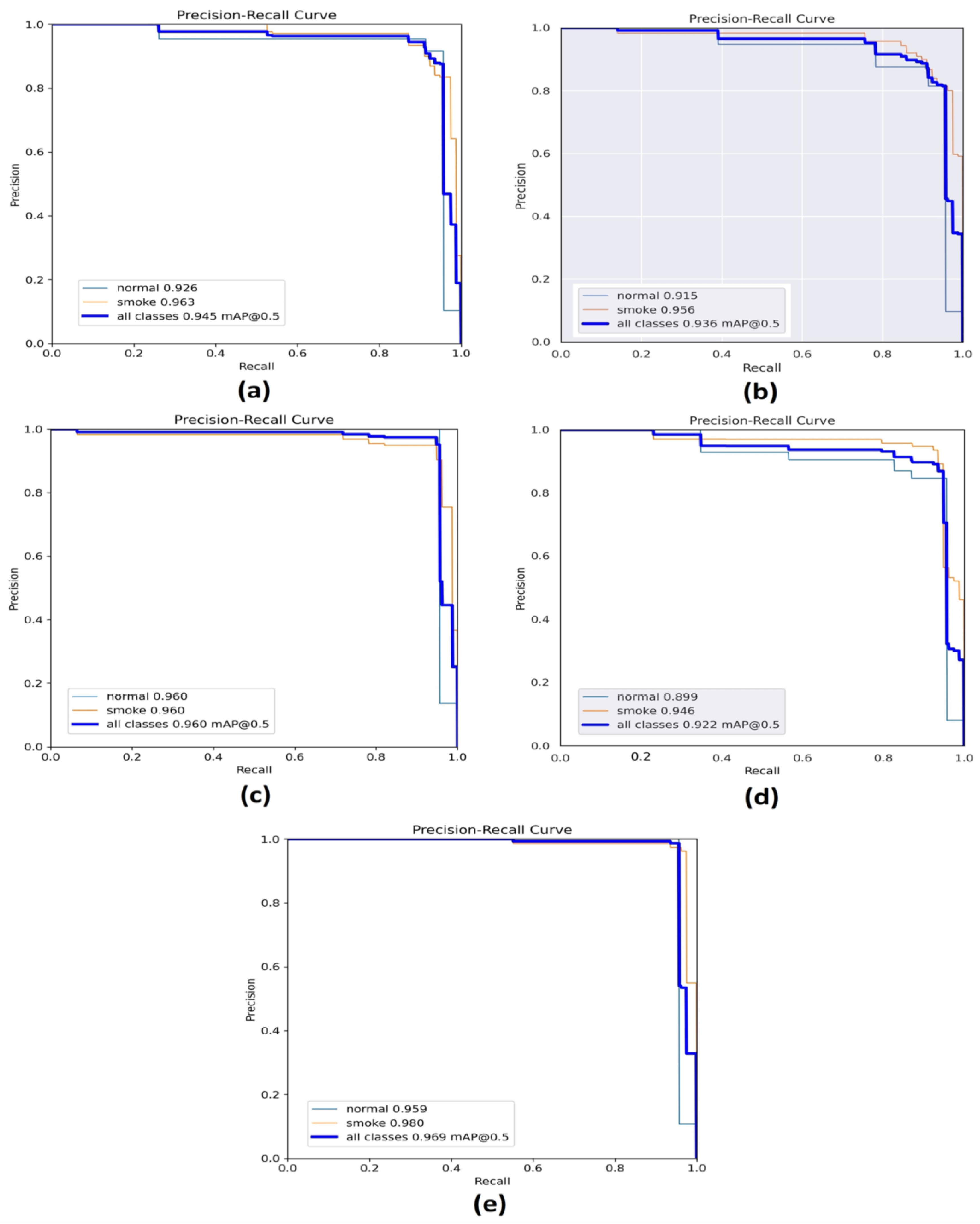
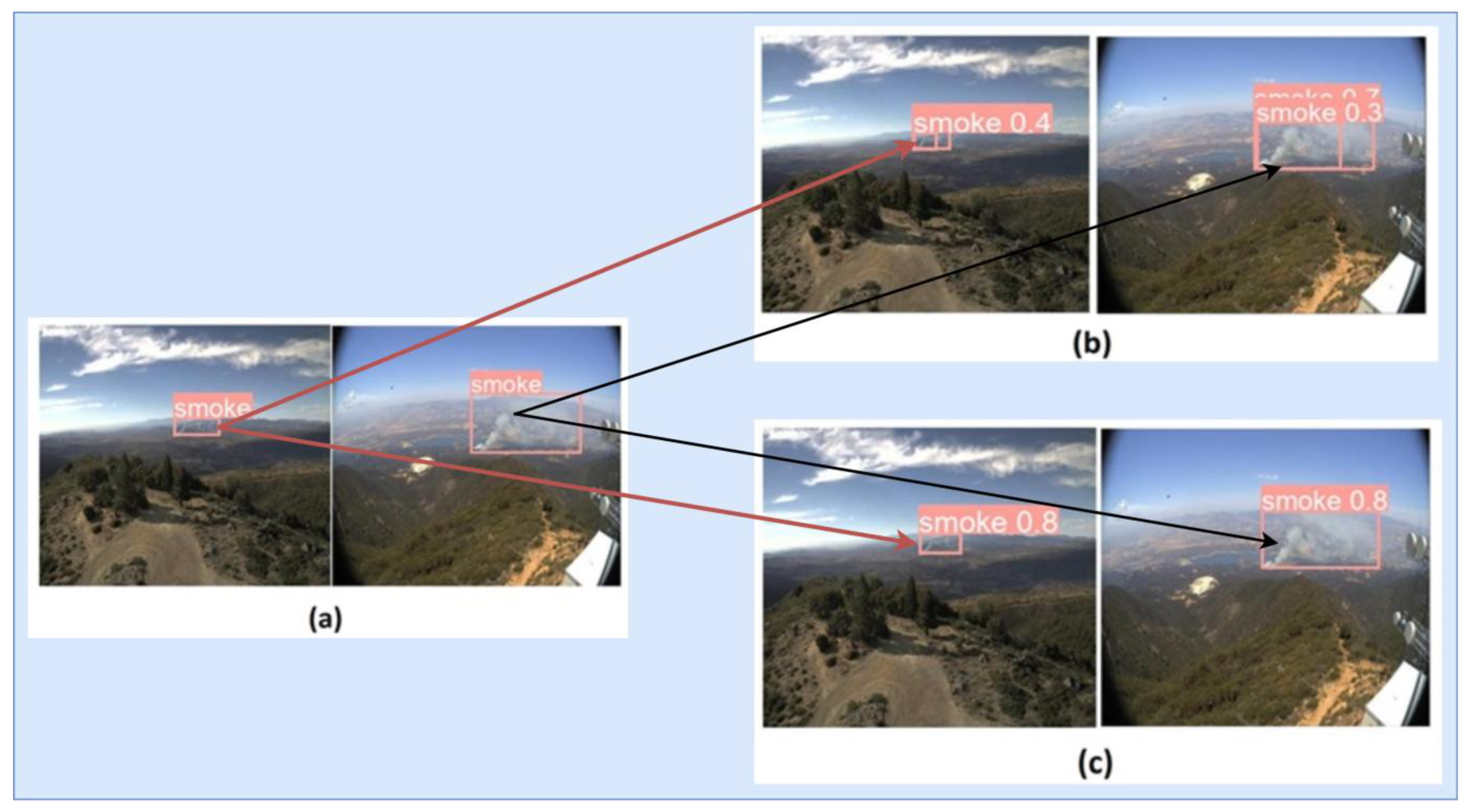
4. Experimental Results
Comparison of the Proposed Model and the Original Model
5. Discussion
6. Conclusions
Funding
Institutional Review Board Statement
Informed Consent Statement
Data Availability Statement
Conflicts of Interest
List of Abbreviations
| GFLOPs | Giga Floating-Point Operations Per Second |
| FPN | Feature Pyramid Networks |
| PAFPN | Path Aggregation Network for Instance Segmentation |
| AP | Average Precision |
| CNN | Convolutional Neural Networks |
| RCNN | Region Convolutional Neural Network |
| YOLO | You Only Look Once |
| AI | Artificial Intelligence |
| ANN | Artificial Neural Networks |
| ML | Machine Learning |
| DL | Deep Learning |
| CV | Computer Vision |
| NMS | Non-Maximum Suppression |
| BN | Batch Normalization |
| mAP | Mean Average Precision |
| RPN | Region Proposal Network |
| SSD | Single Shot MultiBox Detector |
| SPP | Spatial Pyramid Pooling |
| SPPF | Spatial Pyramid Pooling Fast |
| IoU | Intersection Over Union |
| CSP | Cross-Stage Partial Connections |
| PANet | Path Aggregation Network |
| SiLU | Sigmoid Linear Unit |
| ReLU | Rectified Linear Unit |
| IoT | Internet of Things |
| CBS | Composed of Convolution |
| ResNet | Residual Network |
| SGD | Stochastic Gradient Descent |
| TP | True Positives |
| TN | True Negatives |
| FP | False Positives |
| FN | False Negatives |
| PR | Precision Recall |
References
- Dölarslan, M.; Gül, E. Sadece Bir Yangın mı? Ekolojik ve Sosyo-Ekonomik Açıdan Orman Yangınları. Türk Bilimsel Derlemeler Derg. 2017, 10, 32–35. [Google Scholar]
- Eisenman, D.P.; Galway, L.P. The Mental Health and Well-Being Effects of Wildfire Smoke: A Scoping Review. BMC Public Health 2022, 22, 2274. [Google Scholar] [CrossRef]
- Sanderfoot, O.V.; Bassing, S.B.; Brusa, J.L.; Emmet, R.L.; Gillman, S.J.; Swift, K.; Gardner, B. A Review of the Effects of Wildfire Smoke on the Health and Behavior of Wildlife. Environ. Res. Lett. 2022, 16, 123003. [Google Scholar] [CrossRef]
- Meier, S.; Elliott, R.J.R.; Strobl, E. The Regional Economic Impact of Wildfires: Evidence from Southern Europe. J. Environ. Econ. Manag. 2023, 118, 102787. [Google Scholar] [CrossRef]
- Hoover, K.; Hanson, L.A. Wildfire Statistics; CRS In Focus, IF10244; Library of Congress, Congressional Research Service: Washington, DC, USA, 2023. [Google Scholar]
- Shamsoshoara, A.; Afghah, F. Airborne Fire Detection and Modeling Using Unmanned Aerial Vehicles Imagery: Datasets and Approaches. In Handbook of Dynamic Data Driven Applications Systems; Springer: Berlin/Heidelberg, Germany, 2023; Volume 2, pp. 525–550. [Google Scholar]
- Ul Ain Tahir, H.; Waqar, A.; Khalid, S.; Usman, S.M. Wildfire Detection in Aerial Images Using Deep Learning. In Proceedings of the 2022 2nd International Conference on Digital Futures and Transformative Technologies (ICoDT2), Rawalpindi, Pakistan, 24–26 May 2022. [Google Scholar] [CrossRef]
- Zhang, L.; Wang, M.; Ding, Y.; Bu, X. MS-FRCNN: A Multi-Scale Faster RCNN Model for Small Target Forest Fire Detection. Forests 2023, 14, 616. [Google Scholar] [CrossRef]
- Lin, J.; Lin, H.; Wang, F. STPM_SAHI: A Small-Target Forest Fire Detection Model Based on Swin Transformer and Slicing Aided Hyper Inference. Forests 2022, 13, 1603. [Google Scholar] [CrossRef]
- Choutri, K.; Fadloun, S.; Lagha, M.; Bouzidi, F.; Charef, W. Forest Fire Detection Using IoT Enabled UAV and Computer Vision. In Proceedings of the 2022 International Conference on Artificial Intelligence of Things (ICAIoT), Istanbul, Turkey, 29–30 December 2022. [Google Scholar]
- Li, Y.; Rong, L.; Li, R.; Xu, Y. Fire Object Detection Algorithm Based on Improved YOLOv3-Tiny. In Proceedings of the 2022 7th International Conference on Cloud Computing and Big Data Analytics (ICCCBDA), Chengdu, China, 22–24 April 2022; pp. 264–269. [Google Scholar] [CrossRef]
- Huang, T.S.; Schreiber, W.F.; Tretiak, O.J. Image Processing. Proc. IEEE 1971, 59, 1586–1609. [Google Scholar] [CrossRef]
- Kaul, V.; Enslin, S.; Gross, S.A. History of Artificial Intelligence in Medicine. Gastrointest. Endosc. 2020, 92, 807–812. [Google Scholar] [CrossRef]
- Shinde, P.P.; Shah, S. A Review of Machine Learning and Deep Learning Applications. In Proceedings of the 2018 Fourth International Conference on Computing Communication Control and Automation (ICCUBEA), Pune, India, 16–18 August 2018. [Google Scholar] [CrossRef]
- Open Wildfire Smoke Datasets. Available online: https://github.com/aiformankind/wildfire-smoke-dataset (accessed on 11 September 2023).
- Wildfire Dataset Download Link. November 2024. Available online: https://zenodo.org/records/14218779 (accessed on 25 November 2024).
- Zhou, X.; Koltun, V.; Krähenbühl, P. Probabilistic two-stage detection. arXiv 2021, arXiv:2103.07461. [Google Scholar]
- Redmon, J.; Divvala, S.; Girshick, R.; Farhadi, A. You Only Look Once: Unified, Real-Time Object Detection. In Proceedings of the 2016 IEEE Conference on Computer Vision and Pattern Recognition (CVPR), Las Vegas, NV, USA, 27–30 June 2016; pp. 779–788. [Google Scholar] [CrossRef]
- Jiang, P.; Ergu, D.; Liu, F.; Cai, Y.; Ma, B. A Review of YOLO Algorithm Developments. Procedia Comput. Sci. 2022, 199, 1066–1073. [Google Scholar] [CrossRef]
- Terven, J.; Córdova-Esparza, D.-M.; Romero-González, J.-A. A Comprehensive Review of YOLO Architectures in Computer Vision: From YOLOv1 to YOLOv8 and YOLO-NAS. Mach. Learn. Knowl. Extr. 2023, 5, 1680–1716. [Google Scholar] [CrossRef]
- Neubeck, A.; Van Gool, L. Efficient Non-Maximum Suppression. In Proceedings of the 18th International Conference on Pattern Recognition (ICPR’06), Hong Kong, China, 20–24 August 2006; Volume 3, pp. 850–855. [Google Scholar] [CrossRef]
- Girshick, R. Fast R-CNN. In Proceedings of the 2015 IEEE International Conference on Computer Vision (ICCV), Santiago, Chile, 7–13 December 2015; pp. 1440–1448. [Google Scholar]
- Redmon, J.; Farhadi, A. YOLO9000: Better, Faster, Stronger. In Proceedings of the 2017 IEEE Conference on Computer Vision and Pattern Recognition (CVPR), Honolulu, HI, USA, 21–26 July 2017; pp. 6517–6525. [Google Scholar] [CrossRef]
- Liu, W.; Anguelov, D.; Erhan, D.; Szegedy, C.; Reed, S.; Fu, C.Y.; Berg, A.C. SSD: Single Shot MultiBox Detector. Lect. Notes Comput. Sci. 2015, 9905, 21–37. [Google Scholar] [CrossRef]
- Bochkovskiy, A.; Wang, C.Y.; Liao, H.Y.M. YOLOv4: Optimal speed and accuracy of object detection. arXiv 2020, arXiv:2004.10934. [Google Scholar]
- Misra, D. Mish: A self regularized non-monotonic activation function. arXiv 2019, arXiv:1908.08681. [Google Scholar]
- Hussain, M. YOLO-v1 to YOLO-v8, the Rise of YOLO and Its Complementary Nature Toward Digital Manufacturing and Industrial Defect Detection. Machines 2023, 11, 677. [Google Scholar] [CrossRef]
- Jocher, G.; Chaurasia, A.; Stoken, A.; Borovec, J.; NanoCode012; Kwon, Y.; Michael, K.; TaoXie; Fang, J.; Imyhxy; et al. ultralytics/yolov5: v7.0-yolov5 Sota Realtime Instance Segmentation, V7; Zenodo: Geneva, Switzerland, 2022. [Google Scholar] [CrossRef]
- Nepal, U.; Eslamiat, H. Comparing YOLOv3, YOLOv4 and YOLOv5 for Autonomous Landing Spot Detection in Faulty UAVs. Sensors 2022, 22, 464. [Google Scholar] [CrossRef] [PubMed]
- Li, C.; Li, L.; Jiang, H.; Weng, K.; Geng, Y.; Li, L.; Ke, Z.; Li, Q.; Cheng, M.; Nie, W.; et al. YOLOv6: A single-stage object detection framework for industrial applications. arXiv 2022, arXiv:2209.02976. [Google Scholar]
- Wang, C.-Y.; Bochkovskiy, A.; Liao, H.-Y.M. YOLOv7: Trainable Bag-of-Freebies Sets New State-of-the-Art for Real-Time Object Detectors. In Proceedings of the 2023 IEEE/CVF Conference on Computer Vision and Pattern Recognition (CVPR), Vancouver, BC, Canada, 17–24 June 2023; pp. 7464–7475. [Google Scholar] [CrossRef]
- Hussain, M.; Al-Aqrabi, H.; Munawar, M.; Hill, R.; Alsboui, T. Domain Feature Mapping with YOLOv7 for Automated Edge-Based Pallet Racking Inspections. Sensors 2022, 22, 6927. [Google Scholar] [CrossRef]
- Rangari, A.P.; Chouthmol, A.R.; Kadadas, C.; Pal, P.; Singh, S.K. Deep Learning Based Smart Traffic Light System Using Image Processing with YOLOv7. In Proceedings of the 2022 4th International Conference on Circuits, Control, Communication and Computing (I4C), Bangalore, India, 21–23 December 2022; pp. 129–132. [Google Scholar] [CrossRef]
- Gillani, I.S.; Munawar, M.R.; Talha, M.; Azhar, S.; Mashkoor, Y.; Uddin, M.S.; Zafar, U. Yolov5, Yolo-x, Yolo-r, Yolov7 Performance Comparison: A Survey. Comput. Sci. Inf. Technol. (CS & IT) 2022, 12, 17. [Google Scholar] [CrossRef]
- Bist, R.B.; Subedi, S.; Yang, X.; Chai, L. A Novel YOLOv6 Object Detector for Monitoring Piling Behavior of Cage-Free Laying Hens. AgriEngineering 2023, 5, 905–923. [Google Scholar] [CrossRef]
- Kawade, V.; Naikwade, V.; Bora, V.; Chhabria, S. A Comparative Analysis of Deep Learning Models and Conventional Approaches for Osteoporosis Detection in Hip X-Ray Images. In Proceedings of the 2023 World Conference on Communication & Computing (WCONF), Raipur, India, 14–16 July 2023; pp. 1–7. [Google Scholar]
- Xiao, B.; Nguyen, M.; Yan, W.Q. Fruit Ripeness Identification Using YOLOv8 Model. Multimed. Tools Appl. 2023, 83, 28039–28056. [Google Scholar] [CrossRef]
- Passa, R.S.; Nurmaini, S.; Rini, D.P. YOLOv8 Based on Data Augmentation for MRI Brain Tumor Detection. Sci. J. Inform. 2023, 10, 363–370. [Google Scholar] [CrossRef]
- Reis, D.; Kupec, J.; Hong, J.; Daoudi, A. Real-Time Flying Object Detection with YOLOv8. arXiv 2023, arXiv:2305.09972v1. [Google Scholar]
- He, K.; Zhang, X.; Ren, S.; Sun, J. Deep Residual Learning for Image Recognition. In Proceedings of the 2016 IEEE Conference on Computer Vision and Pattern Recognition (CVPR), Las Vegas, NV, USA, 27–30 June 2016; pp. 770–778. [Google Scholar] [CrossRef]
- Bankar, A.; Shinde, R.; Bhingarkar, S. Impact of Image Translation Using Generative Adversarial Networks for Smoke Detection. In Proceedings of the 2021 International Conference on Computational Performance Evaluation (ComPE), Shillong, India, 1–3 December 2021; pp. 246–255. [Google Scholar] [CrossRef]
- Al-Smadi, Y.; Alauthman, M.; Al-Qerem, A.; Aldweesh, A.; Quaddoura, R.; Aburub, F.; Mansour, K.; Alhmiedat, T. Early Wildfire Smoke Detection Using Different YOLO Models. Machines 2023, 11, 246. [Google Scholar] [CrossRef]
- Redmon, J. Yolov3: An incremental improvement. arXiv 2018, arXiv:1804.02767. [Google Scholar]
- Zhang, M.; Tian, X. Transformer Architecture Based on Mutual Attention for Image-Anomaly Detection. Virtual Real. Intell. Hardw. 2023, 5, 57–67. [Google Scholar] [CrossRef]
- Zheng, H.; Duan, J.; Dong, Y.; Liu, Y. Real-time fire detection algorithms running on small embedded devices based on MobileNetV3 and YOLOv4. Fire Ecol. 2023, 19, 31. [Google Scholar] [CrossRef]


| Works’ Details | Algorithms | Limitations |
|---|---|---|
| UI Ain Tahir et al. [7] performed fire detection by taking images from FireNet and FLAME datasets. Images taken from two datasets contain two classes: feverish and non-feverish. In total, 457 images were used in training the Yolov5 algorithm. The model was tested with 65 images. As a result of these stages, the F1 score of the algorithm was found to be 94.44%. | Yolov5 | Low generalization capacity, only one model |
| Zhang et al. [8] detected forest fire using the FLAME dataset. There are 2003 image data in the dataset. In total, 85% of the image data was used for training and 15% was used for testing. For object detection, ResNet50 was used by changing the backbone part of the Faster R-CNN. In training the algorithm with the image data, a MAP value of 85.2% was reached. | Faster R-CNN | Low generalization capacity, only one hybrid model |
| A dataset [9] was created with images collected by the university and from the internet. In total, 90% of the resulting dataset is reserved for training and 10% for testing. The Mask R-CNN algorithm was replaced with the Swin Transformer backbone network. Additionally, PAFPN was used instead of the FPN structure used in Mask R-CNN. As a result of these changes made in the algorithm, an AP value of 89.4% was reached. | Mask R-CNN | Single backbone and algorithm in the model |
| Choutri et al. [10] used 2906 images manually tagged with the FLAME dataset. For forest fire detection, image data is classified as fire and non-fire. Yolov4 was run over 30 epochs and the training time was 14 h, and the AP value was 86%. Yolov2 was run over 60 epochs and the training time lasted 35 h. In total, 85% AP value was obtained from the training set. Faster R-CNN was run over 100 epochs and the training time lasted 60 h. In total, a 66% AP value was obtained from the training set. The SSD was run over 90 epochs and the training time lasted 72 h. In total, a 42% AP value was obtained from the training set. | Yolov4, Yolov2, Faster R-CNN, SSD | Training time is high with different models, AP values are unbalanced |
| Li et al. [11] created a dataset consisting of 3395 images collected from open-source websites. In total, 80% of the data in the dataset was reserved for training and 20% for testing. Some adjustments were made to the Yolov3-tiny model for fire detection. First, a 52 × 52 output layer was added to the FPN network. Then, the SE module was added behind the detection layers. Finally, the first 4 max pooling layers of the backbone structure were replaced with 3 × 3 convolution layers with two steps. After the modified Yolov3-tiny model was trained with the dataset, an 80.8% mAp value was obtained. In the original SSD, Yolov3, Yolov3-tiny, and Yolov4 models, mAp values of 62.1%, 76.5%, 74.9%, and 60.1% were obtained, respectively. | SSD, Yolov3, Yolov3-tiny, Yolov4-tiny | Current algorithms with different models are not included |
| Models | Backbone | Precision | Recall | F1 | mAP |
|---|---|---|---|---|---|
| Yolov5-n | Yolov5 | 0.957 | 0.946 | 0.951 | 0.973 |
| Yolov5-n | EfficientNet_b1 | 0.920 | 0.914 | 0.916 | 0.953 |
| Yolov5-n | MobileNetV3s | 0.926 | 0.931 | 0.928 | 0.959 |
| Yolov5-n | ResNet34 | 0.929 | 0.942 | 0.935 | 0.958 |
| Yolov5-n | ResNet50 | 0.980 | 0.964 | 0.971 | 0.986 |
| Yolov5-s | Yolov5 | 0.950 | 0.940 | 0.944 | 0.956 |
| Yolov5-s | EfficientNet_b1 | 0.907 | 0.894 | 0.900 | 0.946 |
| Yolov5-s | MobileNetV3s | 0.965 | 0.931 | 0.947 | 0.961 |
| Yolov5-s | ResNet34 | 0.877 | 0.836 | 0.856 | 0.908 |
| Yolov5-s | ResNet50 | 0.963 | 0.960 | 0.961 | 0.976 |
| Yolov5-m | Yolov5 | 0.962 | 0.958 | 0.959 | 0.988 |
| Yolov5-m | EfficientNet_b1 | 0.814 | 0.791 | 0.802 | 0.905 |
| Yolov5-m | MobileNetV3s | 0.982 | 0.905 | 0.941 | 0.969 |
| Yolov5-m | ResNet34 | 0.911 | 0.894 | 0.902 | 0.932 |
| Yolov5-m | ResNet50 | 0.941 | 0.973 | 0.956 | 0.971 |
| Yolov5-l | Yolov5 | 0.967 | 0.980 | 0.973 | 0.986 |
| Yolov5-l | EfficientNet_b1 | 0.786 | 0.834 | 0.809 | 0.878 |
| Yolov5-l | MobileNetV3s | 0.956 | 0.932 | 0.947 | 0.974 |
| Yolov5-l | ResNet34 | 0.915 | 0.820 | 0.864 | 0.941 |
| Yolov5-l | ResNet50 | 0.977 | 0.950 | 0.963 | 0.972 |
| Yolov5-x | Yolov5 | 0.971 | 0.932 | 0.951 | 0.982 |
| Yolov5-x | EfficientNet_b1 | 0.944 | 0.918 | 0.930 | 0.957 |
| Yolov5-x | MobileNetV3s | 0.964 | 0.942 | 0.952 | 0.963 |
| Yolov5-x | ResNet34 | 0.923 | 0.931 | 0.926 | 0.963 |
| Yolov8-n | Yolov8 | 0.908 | 0.918 | 0.912 | 0.950 |
| Yolov8-s | Yolov8 | 0.940 | 0.940 | 0.940 | 0.959 |
| Yolov8-m | Yolov8 | 0.914 | 0.953 | 0.933 | 0.965 |
| Yolov8-l | Yolov8 | 0.882 | 0.870 | 0.875 | 0.917 |
| Yolov8-x | Yolov8 | 0.888 | 0.831 | 0.858 | 0.928 |
| Proposed Model | 0.988 | 0.967 | 0.977 | 0.973 |
| Models | Backbone | Precision | Recall | F1 | mAP |
|---|---|---|---|---|---|
| Yolov5-n | Yolov5 | 0.955 | 0.953 | 0.953 | 0.947 |
| Yolov5-n | EfficientNet_b1 | 0.940 | 0.865 | 0.900 | 0.934 |
| Yolov5-n | MobileNetV3s | 0.917 | 0.879 | 0.897 | 0.924 |
| Yolov5-n | ResNet34 | 0.844 | 0.881 | 0.862 | 0.913 |
| Yolov5-n | ResNet50 | 0.945 | 0.959 | 0.951 | 0.960 |
| Yolov5-s | Yolov5 | 0.895 | 0.906 | 0.900 | 0.910 |
| Yolov5-s | EfficientNet_b1 | 0.838 | 0.873 | 0.855 | 0.930 |
| Yolov5-s | MobileNetV3s | 0.945 | 0.920 | 0.932 | 0.942 |
| Yolov5-s | ResNet34 | 0.784 | 0.840 | 0.811 | 0.878 |
| Yolov5-s | ResNet50 | 0.919 | 0.959 | 0.938 | 0.965 |
| Yolov5-m | Yolov5 | 0.926 | 0.953 | 0.939 | 0.960 |
| Yolov5-m | EfficientNet_b1 | 0.699 | 0.785 | 0.739 | 0.820 |
| Yolov5-m | MobileNetV3s | 0.913 | 0.939 | 0.925 | 0.939 |
| Yolov5-m | ResNet34 | 0.817 | 0.897 | 0.855 | 0.907 |
| Yolov5-m | ResNet50 | 0.939 | 0.967 | 0.952 | 0.956 |
| Yolov5-l | Yolov5 | 0.939 | 0.940 | 0.939 | 0.945 |
| Yolov5-l | EfficientNet_b1 | 0.611 | 0.852 | 0.711 | 0.797 |
| Yolov5-l | MobileNetV3s | 0.940 | 0.959 | 0.949 | 0.956 |
| Yolov5-l | ResNet34 | 0.791 | 0.884 | 0.834 | 0.905 |
| Yolov5-l | ResNet50 | 0.937 | 0.928 | 0.932 | 0.960 |
| Yolov5-x | Yolov5 | 0.895 | 0.940 | 0.916 | 0.945 |
| Yolov5-x | EfficientNet_b1 | 0.845 | 0.929 | 0.884 | 0.936 |
| Yolov5-x | MobileNetV3s | 0.950 | 0.944 | 0.946 | 0.960 |
| Yolov5-x | ResNet34 | 0.864 | 0.919 | 0.890 | 0.922 |
| Yolov8-n | Yolov8 | 0.884 | 0.918 | 0.900 | 0.942 |
| Yolov8-s | Yolov8 | 0.856 | 0.927 | 0.890 | 0.926 |
| Yolov8-m | Yolov8 | 0.825 | 0.908 | 0.864 | 0.897 |
| Yolov8-l | Yolov8 | 0.821 | 0.850 | 0.835 | 0.865 |
| Yolov8-x | Yolov8 | 0.844 | 0.824 | 0.833 | 0.856 |
| Proposed Model | 0.954 | 0.964 | 0.958 | 0.969 |
| Models | Backbone | Training Time (h) | Model Size (MB) |
|---|---|---|---|
| Yolov5-n | Yolov5 | 0.21 | 3.9 |
| Yolov5-n | EfficientNet_b1 | 0.69 | 13.8 |
| Yolov5-n | MobileNetV3s | 0.22 | 4.7 |
| Yolov5-n | ResNet34 | 0.51 | 45.3 |
| Yolov5-n | ResNet50 | 0.79 | 55.6 |
| Yolov5-s | Yolov5 | 0.30 | 14.4 |
| Yolov5-s | EfficientNet_b1 | 0.73 | 19.5 |
| Yolov5-s | MobileNetV3s | 0.25 | 9.7 |
| Yolov5-s | ResNet34 | 0.53 | 50.3 |
| Yolov5-s | ResNet50 | 0.85 | 62.5 |
| Yolov5-m | Yolov5 | 0.58 | 42.2 |
| Yolov5-m | EfficientNet_b1 | 0.88 | 32.8 |
| Yolov5-m | MobileNetV3s | 0.31 | 22.3 |
| Yolov5-m | ResNet34 | 0.62 | 62.9 |
| Yolov5-m | ResNet50 | 0.95 | 76.8 |
| Yolov5-l | Yolov5 | 0.97 | 92.9 |
| Yolov5-l | EfficientNet_b1 | 0.95 | 56.2 |
| Yolov5-l | MobileNetV3s | 0.42 | 44.9 |
| Yolov5-l | ResNet34 | 0.73 | 85.5 |
| Yolov5-l | ResNet50 | 1.06 | 101.3 |
| Yolov5-x | Yolov5 | 1.58 | 173.1 |
| Yolov5-x | EfficientNet_b1 | 1.12 | 92.7 |
| Yolov5-x | MobileNetV3s | 0.63 | 80.7 |
| Yolov5-x | ResNet34 | 0.90 | 121.3 |
| Yolov8-n | Yolov8 | 0.22 | 6.2 |
| Yolov8-s | Yolov8 | 0.36 | 22.5 |
| Yolov8-m | Yolov8 | 0.72 | 52.0 |
| Yolov8-l | Yolov8 | 1.08 | 87.6 |
| Yolov8-x | Yolov8 | 1.75 | 136.7 |
| Proposed Model | 1.22 | 138.9 |
| Models | Backbone | Layers | Parameters (M) | GFLOPs |
|---|---|---|---|---|
| Yolov5-n | Yolov5 | 157 | 1.7 | 4.1 |
| Yolov5-n | EfficientNet_b1 | 513 | 6.5 | 11.7 |
| Yolov5-n | MobileNetV3s | 287 | 2.1 | 3.1 |
| Yolov5-n | ResNet34 | 197 | 22.4 | 61.9 |
| Yolov5-n | ResNet50 | 232 | 27.5 | 72.1 |
| Yolov5-s | Yolov5 | 157 | 7.0 | 15.8 |
| Yolov5-s | EfficientNet_b1 | 513 | 9.4 | 16.2 |
| Yolov5-s | MobileNetV3s | 287 | 4.6 | 7.2 |
| Yolov5-s | ResNet34 | 197 | 24.9 | 66.2 |
| Yolov5-s | ResNet50 | 232 | 30.9 | 77.7 |
| Yolov5-m | Yolov5 | 212 | 20.8 | 47.9 |
| Yolov5-m | EfficientNet_b1 | 533 | 16.0 | 27.9 |
| Yolov5-m | MobileNetV3s | 307 | 10.8 | 18.7 |
| Yolov5-m | ResNet34 | 217 | 31.2 | 77.8 |
| Yolov5-m | ResNet50 | 252 | 38.1 | 90.5 |
| Yolov5-l | Yolov5 | 267 | 46.1 | 107.7 |
| Yolov5-l | EfficientNet_b1 | 553 | 27.7 | 49.6 |
| Yolov5-l | MobileNetV3s | 327 | 22.1 | 40.0 |
| Yolov5-l | ResNet34 | 237 | 42.5 | 99.3 |
| Yolov5-l | ResNet50 | 272 | 50.3 | 113.3 |
| Yolov5-x | Yolov5 | 322 | 86.1 | 203.8 |
| Yolov5-x | EfficientNet_b1 | 573 | 45.9 | 84.4 |
| Yolov5-x | MobileNetV3s | 347 | 40.0 | 74.5 |
| Yolov5-x | ResNet34 | 257 | 60.3 | 133.8 |
| Yolov8-n | Yolov8 | 168 | 3.0 | 8.7 |
| Yolov8-s | Yolov8 | 168 | 11.1 | 28.6 |
| Yolov8-m | Yolov8 | 218 | 25.8 | 78.9 |
| Yolov8-l | Yolov8 | 268 | 43.6 | 165.2 |
| Yolov8-x | Yolov8 | 268 | 68.1 | 257.8 |
| Proposed Model | 292 | 69.1 | 149.1 |
Disclaimer/Publisher’s Note: The statements, opinions and data contained in all publications are solely those of the individual author(s) and contributor(s) and not of MDPI and/or the editor(s). MDPI and/or the editor(s) disclaim responsibility for any injury to people or property resulting from any ideas, methods, instructions or products referred to in the content. |
© 2025 by the author. Licensee MDPI, Basel, Switzerland. This article is an open access article distributed under the terms and conditions of the Creative Commons Attribution (CC BY) license (https://creativecommons.org/licenses/by/4.0/).
Share and Cite
Çınarer, G. Hybrid Backbone-Based Deep Learning Model for Early Detection of Forest Fire Smoke. Appl. Sci. 2025, 15, 7178. https://doi.org/10.3390/app15137178
Çınarer G. Hybrid Backbone-Based Deep Learning Model for Early Detection of Forest Fire Smoke. Applied Sciences. 2025; 15(13):7178. https://doi.org/10.3390/app15137178
Chicago/Turabian StyleÇınarer, Gökalp. 2025. "Hybrid Backbone-Based Deep Learning Model for Early Detection of Forest Fire Smoke" Applied Sciences 15, no. 13: 7178. https://doi.org/10.3390/app15137178
APA StyleÇınarer, G. (2025). Hybrid Backbone-Based Deep Learning Model for Early Detection of Forest Fire Smoke. Applied Sciences, 15(13), 7178. https://doi.org/10.3390/app15137178