Abstract
Malicious software presents significant challenges in cybersecurity, leveraging rapidly evolving technologies to bypass traditional defense mechanisms. This research introduces a novel image-based malware classification framework that uses hybrid-model Convolutional Neural Networks to process RGB images generated from assembly code. We present MalevisAsm, an enriched dataset that merges MaleVis malware samples with benign files, and propose a hybrid deep learning model that combines EfficientNetB0 and DenseNet121 for robust feature extraction. The approach transforms Portable Executable files into assembly code, maps opcode transitions into three-channel images, and uses a fine-tuned CNN to classify malware families. Additionally, we implemented Uniform Manifold Approximation and Projection a contemporary nonlinear dimensionality reduction technique, to enhance the identification of previously unseen malware samples via binary classification. Our experiments achieve a top-tier accuracy of 98.45%, surpassing existing benchmarks on the MaleVis dataset. This research contributes to the field by integrating static binary analysis with advanced computer vision techniques, offering a scalable and effective solution for malware detection.
1. Introduction
Malware is malicious software designed to disrupt systems, steal sensitive information, or gain unauthorized access to resources. According to AV-TEST Institute’s 2024 malware statistics report, global malware incidents reached approximately 921 billion cases annually [1]. Malware includes various types such as worms, viruses, bots, trojans, ransomware, spyware, adware, spam and scams. The complexity and adaptability of malware types have made traditional detection methods less effective [2]. Due to the inherent complexity of modern malicious code constructs and evasion techniques, computational and methodological challenges of effective malware classification remain.
Malware analysis employs three core techniques: static analysis (inspecting code without execution), dynamic analysis (monitoring runtime behavior in sandboxed environments), and memory analysis (examining volatile memory artifacts) [3]. While static methods offer efficiency, dynamic approaches reveal actual malicious behaviors, and memory analysis detects advanced evasion techniques, collectively forming a layered defense against evolving threats. As established by [3], malware signatures utilize distinctive algorithmic patterns or hash values to identify specific threats without requiring execution, enabling resource efficiency and rapid detection. However, such static methods exhibit critical limitations when confronted with evasion techniques like code obfuscation, encryption, dead code insertion, or register reassignment. These adversarial manipulations frequently lead to substantial and unpredictable declines in detection accuracy, compromising the reliability of purely signature-based approaches. In contrast to static analysis, dynamic analysis extracts discriminative patterns by executing suspicious files in controlled environments (e.g., sandboxes or virtual machines) and monitoring their runtime behavior. However, this approach demands significantly greater computational resources (memory and CPU) than static methods. Additionally, certain Portable Executable (PE) files necessitate decompression and unpacking to expose analyzable features, while specialized tools are required to trace malicious activities during execution. Complementing static and dynamic approaches, memory-based analysis—specifically volatile memory forensics (VMF)—has emerged as an increasingly vital malware detection paradigm. VMF operates through two critical phases: (1) acquisition, where kernel drivers or emulators extract physical/virtual memory data into dump files, and (2) analysis, employing advanced techniques like machine learning to identify malware artifacts and behavioral patterns [4,5]. This method excels in detecting fileless malware and advanced evasion tactics that bypass traditional analysis.
The malware detection field has progressively incorporated machine learning (ML) and deep learning (DL) methodologies to identify and categorize malicious software variants with increasing accuracy. ML outperforms statistical approaches in complex prediction problems. ML surpasses statistical methods in predictive tasks. The exponential growth of data in modern systems renders classical ML algorithms increasingly ineffective for meaningful analysis. DL addresses big data challenges in cybersecurity by automating feature extraction—a critical advancement over manual methods in traditional ML. Particularly in malware analysis, computer vision techniques detect minute pattern differences, while DL classifiers self-learn discriminative features without predefined rules. Recent studies have proposed deep learning-based visualization methods that transform malware analysis into an image recognition problem. Samples from the same family exhibit similar textural patterns when converted to images. However, generating high-quality visual representations from binaries remains challenging [4,5]. The prevalent method converts 8-bit binary sequences into grayscale pixels, but size standardization causes critical information loss. Opcode n-gram techniques, meanwhile, disregard important contextual features like operand relationships. For this reason, this study aims to both create malware images using PE files with a large new dataset and to classify them with a hybrid method.
First, PE files are converted into assembly code. Then, the assembly code data is visualized, aiming to classify malware types more accurately and robustly.
The main contributions of this article are as follows:
This study presents an innovative methodology for the visual-based classification task using static analysis. Although various methods address the task of malware classification, there is a lack of a model that effectively visualizes assembly code sequences and classifies different malware families.
This study aims to address this deficiency and proposes a new convolutional architecture based on deep learning. The proposed architecture first converts software into assembly code and then converts these codes into three-channel images. This architecture, which is validated with tests on a new dataset, has made significant contributions to the existing literature.
This study investigates the potential of vision-based approaches and convolutional neural networks (CNNs) for malware detection using a novel dataset. We introduce MalevisAsm, an enhanced dataset created by merging the existing MaleVis collection with newly acquired benign samples. This augmentation improves the model’s generalization capacity for more effective malware threat detection and classification.
This paper is structured as follows: Section 2 provides an overview of existing malware classification approaches. Section 3 presents the rationale behind our proposed methodology. The architectural details and implementation of our model are explained in Section 4. Section 5 evaluates the experimental results and compares them with state-of-the-art methods. The article concludes with a summary of contributions in Section 6. The limitations of the current study are discussed in Section 7.
1.1. Current Challenges in Malware Detection
The cybersecurity landscape faces unprecedented challenges as malicious software continues to evolve at an alarming rate, employing sophisticated techniques to evade traditional detection mechanisms. These challenges necessitate innovative approaches that can adapt to the dynamic nature of modern threats.
1.1.1. Evasion and Obfuscation Techniques
Modern malware employs advanced evasion strategies that significantly complicate detection processes. Code obfuscation techniques, including control flow flattening, instruction substitution, and garbage code insertion, deliberately obscure the true functionality of malicious programs [4]. Polymorphic and metamorphic malware variants dynamically alter their code structure while preserving malicious functionality, creating distinct signatures that bypass signature-based detection systems. Additionally, packing and encryption techniques compress and encrypt malware payloads, making static analysis particularly challenging as the actual malicious code remains hidden until runtime execution.
1.1.2. Limitations of Traditional Analysis Methods
Conventional static analysis approaches face significant limitations when confronting obfuscated binaries. Traditional signature-based detection relies on known patterns and heuristics, rendering it ineffective against zero-day threats and previously unseen malware variants. Dynamic analysis, while capable of observing runtime behavior, suffers from sandbox evasion techniques where malware can detect virtualized environments and remain dormant to avoid detection. Furthermore, the computational overhead associated with comprehensive dynamic analysis makes real-time detection challenging in production environments.
1.1.3. Feature Extraction and Representation Challenges
Extracting meaningful features from Portable Executable (PE) files presents substantial difficulties, particularly when dealing with obfuscated samples. Traditional feature extraction methods often struggle with high-dimensional feature spaces, leading to the curse of dimensionality and reduced classification performance. The heterogeneous nature of malware families further complicates feature selection, as different malware types exhibit varying behavioral patterns and structural characteristics. Additionally, the rapid evolution of malware techniques continuously introduces new features that existing models may not adequately capture [6].
1.1.4. Scalability and Performance Requirements
Modern cybersecurity environments demand real-time detection capabilities capable of processing thousands of samples simultaneously. Traditional machine learning approaches often exhibit limited scalability when confronted with large-scale datasets, leading to increased processing times and reduced effectiveness. The trade-off between detection accuracy and computational efficiency remains a critical challenge, as organizations require both high precision and rapid response times to effectively counter emerging threats.
1.1.5. The Need for Advanced Visualization and Deep Learning
These challenges highlight the necessity for innovative approaches that can effectively bridge the gap between traditional binary analysis and modern machine learning techniques. The transformation of assembly code into visual representations offers a promising avenue for leveraging computer vision advances in malware detection. By converting opcode sequences into RGB images and employing hybrid convolutional neural networks, we can potentially overcome many of the limitations associated with traditional feature extraction methods while maintaining scalability and detection accuracy.
2. Related Work
There is much research on different aspects of malware detection. Practical and effective experimental results in the classification of malware are obtained by using different types of methods. In this section, a brief overview of some studies has been provided particularly those focusing on deep learning-based methods for malware detection.
Catalano et al. [7] explored CNNs for malware detection by converting binaries to grayscale images, achieving 99.77% accuracy on Linux samples but only 86.83% on Windows, highlighting challenges with polymorphic malware. Divakarla et al. [8] proposed a deep neural network for Windows malware classification using the EMBER dataset. Kumar et al. [9] combined texture features (SIFT, KAZE, HOG) with a BoVW model on the Malimg dataset, attaining 98.34% accuracy through ensemble learning.
For advanced threats, Kara et al. [10] analyzed fileless malware via memory forensics, while Gibert et al. [11] evaluated n-gram and deep learning against metamorphic samples from the Microsoft Malware Challenge. Nawaz et al. [12] introduced sequential pattern mining (SPM) for API call analysis, focusing on WannaCry and Zeus variants. Kuriyal et al. [13] achieved 96% accuracy via dynamic API monitoring, and Deng et al. [14] developed the Fantasm framework to study polymorphic malware behavior on bare-metal systems.
Alternative approaches include supervised ML (Selamat et al. [15]), hybrid signature/anomaly detection (Akhtar and Feng [16]), and behavioral modeling (AL-HASHMI et al. [17]). Quebrado et al. [18] proposed a graph-based method for Android malware, outperforming image-based techniques. Ajwani [19] leveraged ontology knowledge graphs, while Sriram et al. [20] employed multi-scale learning with spatial pyramid pooling. Sern et al. [21] introduced BinImg2Vec, combining self-supervised and supervised learning for binary image classification.
According to the analysis principle, it can be discussed in three different classes, as shown in Figure 1. In the static analysis method, the image of the malware before it is executed is analyzed. In the dynamic analysis method, the behavior of the malware and the traces it leaves behind during its execution are analyzed. Memory images and other runtime data also need to be examined. For this reason, Memory-based methods are used.
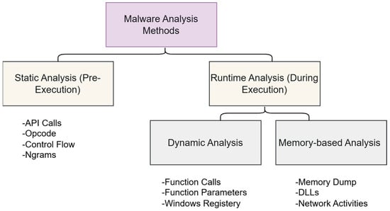
Figure 1.
Malware Analysis Groups in the Literature [22].
2.1. Static Analysis
Static analysis examines software without execution by inspecting Windows API calls, string signatures, control flow graphs, opcodes, and byte sequences. These elements reveal program behavior and malicious intent, particularly through execution flow patterns in control flow graphs and CPU instruction codes. While cost-effective for PE file analysis, the method requires preprocessing steps like unpacking to extract meaningful features. The studies on static analysis in the literature are summarized in Table 1.

Table 1.
Summary of static analysis studies.
Signature-based detection relies on unique byte sequences or hash values to identify known malware samples. However, these methods exhibit zero detection capability against unknown variants and can be easily evaded through simple code modifications such as instruction reordering or NOP insertion [4]. The exponential growth of malware variants also creates scalability challenges requiring continuous signature database updates.
2.2. Dynamic Analysis
Dynamic analysis, or behavioral analysis, executes malware in controlled environments (e.g., sandboxes, VMs) to monitor runtime behavior through function calls, registry changes, network activity, and file system modifications. While effective for detecting hidden threats, this method is resource-intensive and time-consuming. Its success depends on meeting precise execution conditions, as malware may evade analysis in non-native environments. The studies on dynamic analysis in the literature are summarized in Table 2.
Table 2.
Summary of dynamic analysis studies.
Dynamic analysis monitors malware behavior during runtime execution in controlled environments such as sandboxes. While effective at observing actual malicious activities, these methods face significant limitations including sandbox evasion techniques where malware detects virtualized environments and remains dormant [4]. The computational overhead of runtime monitoring makes real-time detection challenging, and time-delayed malware can evade detection by activating after analysis completion.
2.3. Memory-Based Analysis
Memory analysis has gained prominence as it bypasses the limitations of static analysis when facing obfuscated disk data. However, these approaches encounter substantial challenges including the ephemeral nature of memory evidence that can be quickly overwritten or cleared [6]. Advanced malware employs memory evasion techniques such as process hollowing, reflective DLL loading, and fileless attacks that minimize memory footprints, making detection difficult. Unlike disk-based methods, memory retains unencrypted execution artifacts (DLLs, processes, network activities) until system shutdown, enabling the detection of evasive malware. This approach requires no unpacking and operates OS independently, though specialized hardware tools are often needed for reliable acquisition. The studies on memory-based analysis in the literature are summarized in Table 3.
Table 3.
Summary of Memory-Based Analysis Studies.
We contribute to malware detection research in four significant ways:
(1) Novel Assembly-to-RGB Visualization Technique: We introduce a novel Assembly-to-RGB visualization technique that encodes opcode transitions as three-channel matrices, preserving structural semantics lost in grayscale representations. Unlike prior work Nataraj et al. [31], our mapping explicitly separates opcodes (red), operands (green), and control flow (blue) into distinct channels. This approach directly addresses the signature-based detection limitations by creating visual representations that remain consistent despite code modifications, while capturing semantic relationships invisible to traditional byte-sequence analysis.
(2) Hybrid CNN Architecture: We propose a hybrid CNN architecture combining EfficientNetB0 (for local pattern detection) and DenseNet121 (for global feature reuse). This dual-architecture approach overcomes the feature extraction limitations of single-model systems and provides robust detection capabilities against evasion techniques through complementary feature learning mechanisms.
Recent advances in CNN-based malware detection convert binaries into grayscale images for classification, leveraging architectures like VGG or ResNet (Table 1). While these methods outperform traditional approaches, they face three key limitations: (1) Single-architecture designs struggle to generalize across diverse malware families; (2) Feature extraction lacks multi-scale diversity, hindering detection of novel pattern combinations; and (3) Grayscale representations lose critical semantics (e.g., opcode-operand relationships), impairing behavioral analysis (Table 1). Our work addresses these gaps through hybrid CNNs and RGB-based semantic preservation.
(3) Enhanced Dataset Integration: We enhance the MalevisAsm dataset through strategic benign sample integration, balancing classes while maintaining real-world distribution. This addresses the generalization weakness of traditional approaches by providing comprehensive training data that enables better discrimination between malicious and benign patterns.
(4) UMAP-Enhanced Unseen Malware Detection: We demonstrate through UMAP visualization how our approach effectively identifies previously unseen malware samples via advanced dimensionality reduction. This directly tackles the zero-day detection problem that plagues signature-based and memory-based analysis methods, enabling proactive threat identification.
These innovations collectively address critical gaps in interpretable, efficient malware analysis while providing practical solutions to the fundamental limitations of traditional detection approaches including poor generalization, evasion susceptibility, and manual feature engineering bottlenecks.
Table 4 shows in detail the comparison of our model with previous models and the contributions.
Table 4.
Comparative analysis and research gaps.
3. Materials and Methods
This section first presents the collected dataset, followed by a concise overview of the image descriptors employed in our methodology.
3.1. Dataset Description
The dataset contains malware samples of different numbers and families. The state of these samples before conversion is in Portable Executable (PE) form.
This study explores the potential of classifying malware by extracting semantic patterns from code and representing them as images. After validating the methodology with an initial experiment, a deep learning-based classifier was employed to enhance performance. A new dataset, MalevisAsm, was created by combining the MaleVis dataset with benign files to improve the model’s generalization in detecting various malware threats.
The MaleVis (Malware Evaluation with Vision) dataset, publicly released in 2019 by Bozkir et al. [32], contains 14,226 RGB images. The MaleVis dataset, which is available through the link (https://web.cs.hacettepe.edu.tr/~selman/malevis/ accessed on 22 June 2025) provided by the authors, contains only RGB images. In this study, malware exe files based on the MaleVis dataset were used and a different dataset was obtained from the original MaleVis dataset. Although the MaleVis dataset consists of images, it is derived from malware exe files and is therefore domain-specific.
The dataset provides 25 malware classes. The benign class was created by the aggregation method. The benign executable files in our dataset were sourced from two main avenues to ensure both diversity and reliability. One portion was collected from our own clean and actively used Windows systems, including installed software utilities and default system files. The other portion was obtained from trusted and legally permissible open-source platforms such as SourceForge, GitHub between [Start Date January 2025] and [End Date March 2025], and official vendor websites, with an emphasis on widely used, signed, and open-source applications. To verify their benign nature, all files were scanned using multiple reputable antivirus engines, including Windows Defender, and only those with zero detections across all scans were retained. Each file was also tested in sandboxed environments like Windows Sandbox, and those showing any alerts or suspicious behavior were excluded. Additional behavioral checks using tools such as Windows Defender Application Guard were performed for further validation. Files with conflicting antivirus results, rare detection flags, or unsigned origins were removed to reduce the risk of false positives and ensure dataset integrity. In this way, a total of 26 classes were obtained. It contains 15,212 images: 12,091 training images and 3121 validation images. All images are resized to 224 × 224 pixels for uniformity. Table 4 provides example RGB images from the Malevis dataset, highlighting the visual differences between malware classes. Also, Table 5 presents the detailed class distribution of the MalevisAsm dataset. As shown, the dataset exhibits class imbalance with some classes containing significantly fewer samples (e.g., InstallCore.C: 8 samples) compared to others (e.g., Adposhel: 500 samples). This imbalance reflects the real-world distribution of malware families, where certain variants are naturally more prevalent.
Table 5.
MalevisAsm dataset.
3.2. Transfer Learning
Transfer learning repurposes pre-trained neural networks for new tasks by reusing learned features from source domains (e.g., ImageNet). The process involves: (1) replacing the final classification layer to match target task requirements, (2) freezing early layers that detect universal features (edges, textures), and (3) fine-tuning later layers with reduced learning rates. For example, a network trained for general object recognition can be adapted to facial expression analysis by modifying only its last layers while preserving low-level visual detectors. This approach significantly reduces data and computational requirements compared to training from scratch.
Optimization techniques like Adam with carefully tuned learning rates prevent overwriting valuable pre-trained weights. The method works because deep networks learn hierarchical features—fundamental patterns in early layers transfer across domains, while only specialized interpretations need adjustment. Transfer learning has proven particularly effective for computer vision tasks with limited training data.
Three principal transfer learning approaches enable effective model adaptation to new tasks. Fine-tuning represents the most flexible method, where an entire pre-trained network undergoes additional training on target data. This approach works best when source and target domains share significant similarities, though it requires substantial computational resources and risks overfitting with limited data. Partial freezing offers a balanced alternative by keeping early convolutional layers fixed while retraining later layers, preserving generic feature extractors while adapting high-level representations. Progressive learning introduces more sophisticated adaptation through gradual layer unfreezing during training, often incorporating techniques like discrepancy minimization between source and target feature distributions [26,33,34,35]. The effectiveness of these methods stems from the hierarchical nature of deep networks, where early layers develop general features applicable across domains while later layers specialize. Fine-tuning remains most prevalent in practice due to its adaptability, though partial freezing provides superior efficiency for related domains, and progressive methods excel when bridging dissimilar domains. Selection depends on critical factors including dataset size, domain similarity, and available computational resources, with all methods leveraging the fundamental advantage of pre-trained feature representations to accelerate learning in target tasks.
3.3. EfficientNetB0
EfficientNet represents a family of convolutional neural networks specifically optimized to achieve high performance while maintaining parameter efficiency. In this study, we employ the EfficientNetB0 variant as a feature extractor [26,33,34,35], leveraging its ImageNet pretrained weights for transfer learning. The model is implemented without its fully connected layers (include_top = False) and utilizes global average pooling to extract high-level spatial features. To enhance domain adaptation, the final 20 layers were unfrozen during fine-tuning, allowing the network to adjust its deeper feature representations specifically for our malware classification task.
3.4. DenseNet121
DenseNet121 is a deep convolutional neural network architecture that employs dense connections between layers to enhance gradient flow and enable efficient feature reuse [26,33,34,35]. For our implementation, we utilize the model pretrained on ImageNet weights while removing the original classification head (include_top = False) to adapt it for feature extraction. The architecture incorporates global average pooling to generate compact high-level feature representations. To optimize performance for our specific domain, we unfreeze the final 20 layers during fine-tuning, allowing the network to learn specialized feature patterns while preserving the valuable generic features learned from ImageNet.
3.5. Uniform Manifold Approximation and Projection (UMAP)
UMAP (Uniform Manifold Approximation and Projection) is a nonlinear dimensionality reduction technique that leverages manifold learning and algebraic topology to preserve both local and global data structures in low-dimensional embeddings. Unlike linear methods such as PCA, UMAP constructs a high-dimensional graph representation of the data and optimizes a low-dimensional counterpart by minimizing the cross-entropy between topological representations. The algorithm operates through two key phases: (1) computing a fuzzy simplicial set representation of the input data using nearest-neighbor graphs with adaptive kernel bandwidths, and (2) optimizing the low-dimensional embedding through stochastic gradient descent to maintain the topological relationships. Key parameters include n_neighbors, which balances local versus global structure preservation (typically 15–200), and min_dist, controlling cluster compactness (default 0.1). Comparative studies demonstrate UMAP’s superior scalability and preservation of inter-cluster distances relative to t-SNE, particularly for high-dimensional feature spaces like image embeddings or genomic data. In malware analysis, UMAP has proven effective for visualizing hierarchical feature relationships and detecting anomalous patterns [36].
4. Methodology
The methodology consists of three main stages: Data Preprocessing, Convolutional Neural Network (CNN) Design, Classification and Evaluation. For the data preprocessing step, the PE files in the dataset are converted into .asm files. In this model, all .exe files within a folder are processed to generate RGB image output formats. These processes are specifically designed to adapt file formats for different analysis methods, particularly in the context of malware analysis.
The model processes executables first through asm files. It is dedicated to creating .asm files. Subsequently, the .asm files are converted into RGB image files using separate methods.
After these processes, the output locations for the bytes and ASM files are determined while maintaining the original folder structure. The necessary folders are created using “os.makedirs”.
In the next step, classification is performed using a new model with CNN layers, and the results are evaluated. Additionally, UMAP, a dimensionality reduction and multi-faceted learning technique, is used for this study in the context of malware image transformation problems. The general flowchart is shown in Figure 2.
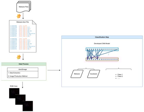
Figure 2.
The proposed model, which processes images represented by their Red, Green, and Blue (RGB) channels.
Explanations regarding the developed model are given under the following headings:
(i) Dataset and Preprocessing
The dataset consists of malware images generated from assembly code files. The dataset is divided into training, validation, and test sets. The training and validation data are loaded using the image_dataset_from_directory function with an 80/-20 split, while the test dataset is loaded separately. To enhance model generalization, data augmentation techniques such as random flipping, rotation, zoom, and contrast adjustments are applied using TensorFlow’s Sequential API.
(ii) Model Architecture
A hybrid deep learning model is designed by combining EfficientNetB0 and DenseNet121 architectures. The models are initialized with pre-trained ImageNet weights and are fine-tuned by unfreezing the last 20 layers. The extracted features from both architectures are concatenated and passed through a series of fully connected layers with batch normalization, dropout, and L2 regularization. The final classification layer contains 26 output neurons with a softmax activation function. The model training is performed in a GPU-accelerated TensorFlow environment. Memory growth settings are enabled for efficient GPU utilization. Training and testing times are recorded to analyze computational performance. The model’s performance is evaluated using the test dataset. Predictions are obtained in batches for efficient memory usage. The evaluation includes accuracy, confusion matrix visualization, and classification reports generated using scikit-learn’s confusion_matrix and classification_report functions.
(iii) Training Configuration
The model is trained using the Adam optimizer with a cosine decay learning rate scheduler. The loss function used is SparseCategoricalCrossentropy, and the evaluation metric is accuracy. Class imbalance is handled by computing class weights using the compute_class_weight function from scikit-learn. The model training includes an early stopping callback to prevent overfitting.
Training history is visualized through accuracy and loss plots over epochs. Additionally, Uniform Manifold Approximation and Projection (UMAP) is used to visualize high-dimensional feature representations in a 2D space.
4.1. Step 1: Data Preprocessing
The study utilizes a dataset of malware images generated from assembly code representations, partitioned into training (80%), validation (20%), and test sets. All images were standardized to 224 × 224-pixel resolution to conform with the input specifications of the implemented neural architectures. To improve model generalizability, an extensive data augmentation pipeline was employed during training, comprising random horizontal flips, 20-degree rotations, 20% zoom transformations, and 20% contrast adjustments. These stochastic transformations artificially expand the training distribution, enhancing robustness against geometric and photometric variations while preserving malicious semantic features. The augmentation strategy effectively simulates real-world variance in malware visual patterns without altering class-discriminative characteristics, as demonstrated in prior work on vision-based malware analysis.
(i) PE to ASM Conversion (PE2Asm):
The machine code is disassembled into assembly (ASM) format using specialized tools such as objdump. Subsequently, opcode transition matrices are computed and transformed into RGB images for further analysis, as illustrated in Figure 3.
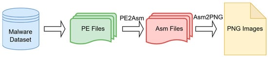
Figure 3.
PE to PNG conversion.
In Figure 4, The convert_to_asm function performs essential machine code to Assembly language conversion, enabling detailed analysis of executable files through human-readable disassembly. This transformation process is particularly valuable for malware analysis and reverse engineering applications, as it reveals the fundamental operational logic of compiled binaries at the processor instruction level. By converting portable executable (.exe) files into their Assembly equivalents (e.g., transforming sample.exe to sample.asm), the function provides security analysts with critical insights into program behavior through three primary aspects: the sequence of processor-level commands being executed, memory access patterns through register operations and address references, and the overall organizational structure of the program including function calls and control flow mechanisms. The implementation leverages the Linux objdump utility with the -d disassembly flag to accurately translate machine instructions into their Assembly representations while maintaining the original program’s structural integrity. To ensure reliable operation during automated analysis pipelines, the function incorporates comprehensive error handling to manage potential issues with corrupted or malformed input files. This disassembly approach forms the foundation for subsequent static analysis phases by exposing low-level implementation details that are critical for understanding malicious functionality, including payload delivery mechanisms, evasion techniques, and system interaction patterns. The methodology aligns with established reverse engineering practices where static disassembly enables both manual code inspection and automated feature extraction for security analysis applications.
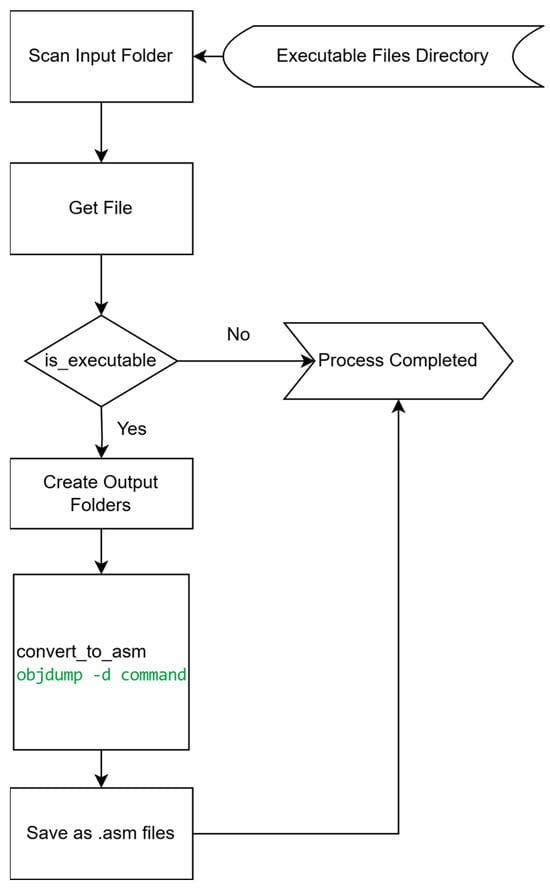
Figure 4.
PE2Asm transformation.
While objdump is primarily associated with Linux (version 2.38, part of the GNU Binutils package) environments, it effectively handles Windows PE files through its Binary File Descriptor (BFD) library support for multiple executable formats. This cross-platform capability has been demonstrated in malware analysis research, where Linux-based tools are commonly employed for analyzing Windows malware samples [As noted in “Obfuscated Malware Detection: Investigating Real-world Scenarios through Memory Analysis”, Ref. [28] cross-platform analysis tools provide valuable flexibility in malware research environments]. However, we acknowledge that our current approach assumes successful disassembly of executable files, which may be limited when dealing with packed or obfuscated malware samples that employ evasion techniques. Integration with automated unpacking tools or hybrid analysis approaches combining static and dynamic methods would be necessary to extend applicability to such challenging samples in real-world scenarios.
In response to reviewer feedback, and to empirically validate the limitations of our static analysis approach, we conducted a comparative experiment. The goal was to assess the performance of objdump—the disassembler used in our pipeline—against a state-of-the-art reverse engineering tool on packed executable files. Packed executables are a common obfuscation technique used by malware to hinder static analysis.
For this test, we created a small set of Windows PE files and packed them using UPX (v5.0.1), a widely known executable packer. We then analyzed these packed samples with both objdump and Ghidra (v11.3.2), a powerful framework developed by the NSA that includes advanced capabilities for handling obfuscated code. The comparison focused on whether the disassembler could look past the packing layer to analyze the original program’s code, specifically by identifying the Original Entry Point (OEP).
As demonstrated in Table 6, objdump was unable to bypass the UPX packing layer. Its output was limited to the disassembly of the packer’s stub code, which is responsible for decompressing the original program in memory at runtime. Consequently, the actual logic of the original application remained inaccessible to our analysis pipeline. In contrast, Ghidra successfully identified the presence of UPX, automatically suggested its built-in unpacking script, and allowed for a full analysis of the original, unpacked code.
Table 6.
Comparative analysis of disassembler performance on UPX-Packed PE files.
This empirical result provides concrete evidence for the limitation discussed in our manuscript: our current methodology is effective on non-obfuscated or unpacked files but would require pre-processing with dedicated unpacking tools to handle evasive malware samples in real-world scenarios.
The example output of objdump typically resembles the following content:
“00401000 <_start>:
401000: 31 ed xor %ebp,%ebp
401002: 49 89 d1 mov %rdx,%r9
401005: 5e pop %rsi
401006: 48 89 e2 mov %rsp,%rdx
401009: 48 83 e4 f0 and $0xfffffffffffffff0,%rsp”
The disassembly output provides critical low-level information for malware analysis, where memory addresses (e.g., 401000) reveal instruction locations and processor operations (e.g., xor, mov) expose malicious functionality. These elements are transformed into a visual representation through a three-channel encoding scheme. The conversion process generates distinct transition matrices capturing different aspects of opcode sequences: the byte transition matrix tracks alphanumeric character patterns across instructions, the opcode transition matrix records initial character sequences, and the quality transition matrix analyzes terminal character relationships. These matrices are mapped to RGB channels (red, green, and blue, respectively), creating composite images that encode the malware’s behavioral patterns. The red channel preserves general character-level transitions, while the green and blue channels emphasize opcode-specific structural relationships. This tripartite representation effectively converts sequential assembly instructions into spatial patterns that simultaneously capture local operation sequences and global code structure, serving as distinctive behavioral fingerprints for classification. The resulting visualizations maintain the semantic relationships inherent in the original code while presenting them in a format amenable to deep learning analysis, particularly for convolutional neural networks designed for image processing.
The assembly files are processed with automatically determined encoding, and the opcode (operation) and operand (parameter) information are extracted. Following this, transition probability matrices for byte, opcode, and quality levels are calculated based on character transitions and then normalized. Three different transition matrices are combined as RGB channels to generate an image. The images are saved in 8-bit RGB format as .png files. With parallel processing, multiple files are processed simultaneously, reducing the processing time, and the status of the tasks is regularly reported. As a result, the RGB images are saved in the specified directory while maintaining the class-based folder structure.
The encoding of the .asm files is automatically determined, ensuring that the files are correctly processed regardless of their initial format. Once the encoding is identified, information about the opcode (operation) and operand (parameter) is extracted from the assembly code.
Transition probability matrices are calculated for byte, opcode, and quality levels based on character transitions within the assembly instructions. These matrices are then normalized to ensure consistent values across the datasets. Afterward, the three transition matrices are combined into RGB channels, resulting in the creation of an image that visually represents the opcode patterns.
The generated images are saved in 8-bit RGB format as .png files, which ensures efficient storage while maintaining image quality. To enhance processing efficiency, multiple files are handled simultaneously through parallel processing, reducing the overall computation time. The status of each processing task is continuously reported to monitor the progress.
The resulting RGB images are saved in the specified directory, organized in a manner that maintains the class-based folder structure. This organization allows for easy access and further analysis of the images.
(ii) ASM to Image Converter (Asm2Image):
This study presents a systematic approach for converting executable byte files into RGB-format PNG images to facilitate the visual analysis of assembly code. MCTVD method was used for Asm2Image transformation [37].
The proposed conversion pipeline comprises several key stages, including assembly file preprocessing, transition matrix computation, image generation, parallel processing, and structured output storage.
As shown in Figure 5, the conversion process involves the following steps:
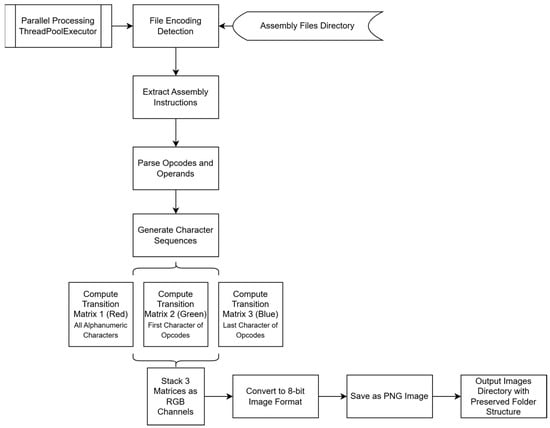
Figure 5.
Asm2Image Transformation.
- (i)
- Assembly File Processing
The system begins by automatically detecting the character encoding of .asm files to ensure accurate text parsing and prevent potential misinterpretation of assembly instructions. This crucial preprocessing step accounts for various encoding formats that may be encountered in different disassembly outputs. Following successful encoding validation, the pipeline performs comprehensive instruction extraction, isolating both opcodes (machine instructions) and their corresponding operands (parameters) from the assembly code. This extraction process meticulously preserves the syntactic structure and semantic relationships within the code, maintaining the original program logic while preparing the data for subsequent analysis stages. The extracted opcode-operand pairs form a complete representation of the executable’s functionality, capturing not just individual operations but their contextual relationships and execution patterns. This dual-level preservation proves particularly valuable for malware analysis, as it enables the reconstruction of both low-level processor commands and higher-level program behavior. The system handles various assembly syntax variations and mnemonics while maintaining consistent output formatting for analysis. Error-checking mechanisms verify the integrity of extracted instructions, flagging any malformed or ambiguous code segments for further inspection. This robust preprocessing ensures that subsequent visualization and classification stages operate on accurate, standardized representations of the original binary’s behavior.
- (ii)
- Transition Matrix Computation and Image Generation
The conversion process involves calculating transition probability matrices at three distinct levels—byte, opcode, and quality—by analyzing sequential character patterns within the assembly code. Each matrix captures the statistical relationships between consecutive elements, with byte-level transitions reflecting raw data patterns, opcode-level transitions revealing instruction sequences, and quality-level transitions encoding structural features of the code. These matrices are then normalized to ensure consistent scaling across different samples, enabling fair comparison and analysis. The normalized matrices are subsequently mapped to the RGB color channels of an image, where the byte, opcode, and quality transitions are represented in the red, green, and blue channels, respectively. This transformation effectively converts the statistical properties of the assembly code into a structured visual representation, preserving both local and global patterns in a format suitable for deep learning-based analysis. The resulting image encapsulates the semantic and syntactic relationships within the original code, facilitating the detection of malware-specific features through computer vision techniques. This approach leverages the discriminative power of color-encoded structural information while maintaining computational efficiency for large-scale datasets.
- (iii)
- Image Storage and Parallel Processing
The system stores the generated malware images in 8-bit RGB PNG format, which provides an optimal balance between image quality and file size efficiency. This standardized format ensures compatibility with common computer vision and deep learning frameworks while preserving the discriminative features encoded in the three-channel visualization. To handle large-scale datasets efficiently, the framework implements parallel processing capabilities that distribute the computational workload across multiple CPU cores. This parallel execution architecture significantly improves processing throughput, enabling the timely analysis of extensive malware collections. The system maintains organized storage by preserving the original directory structure and file naming conventions while incorporating progress tracking and error-handling mechanisms to ensure reliable operation during batch processing. The combination of optimized image compression and parallel computation makes this approach practical for real-world malware analysis scenarios where processing thousands of samples is required.
- (iv)
- Structured Output Organization
The resulting RGB images are stored in a user-defined directory while preserving the original class-based folder hierarchy. This facilitates organized storage, efficient retrieval, and streamlined use in downstream tasks such as classification or clustering.
4.2. Step 2: Classification
Convolutional Neural Networks (CNN) are deep learning algorithms commonly used in image processing, which take images as input. This algorithm, consisting of various layers, captures features from the images using different operations and classifies them accordingly. The image passes through layers such as Convolutional, Pooling, and Fully Connected.
The Convolutional layer is the first layer in CNN algorithms that processes the image. As is known, images are essentially matrices composed of pixels containing specific values. In this layer, a smaller filter, compared to the original image size, slides across the image and attempts to capture certain features from it.
The Pooling layer reduces the input size, which in turn decreases the number of parameters within this activation.
In the Fully Connected layer, the image, which has passed multiple times through convolutional and pooling layers and is in matrix form, is flattened into a vector.
Our proposed model, illustrated in Figure 6, employs a hybrid architecture that synergistically combines two powerful pre-trained convolutional neural networks (CNNs), EfficientNet-B0 and DenseNet-121, to act as parallel feature extractors. This dual-backbone design is motivated by the hypothesis that each network can capture complementary visual patterns from our RGB-encoded malware representations.

Figure 6.
Architecture of the CNN used in the study.
Both backbones were initialized with weights pre-trained on ImageNet. To adapt these models to our specific domain, we applied a fine-tuning strategy where the majority of the layers were kept frozen, while only the final 20 layers of each network were unfrozen and made trainable. This preserves the rich, general-purpose features learned from ImageNet while allowing the model to learn domain-specific features relevant to malware classification.
The feature extraction process for each backbone can be formulated as follows:
where
- x is the input RGB image of size 224 × 224.
- and represent the feature extraction functions of the EfficientNet-B0 and DenseNet-121 backbones, respectively.
- ∈ ℝ1280 is the resulting feature vector from the EfficientNet-B0 branch after Global Average Pooling.
- f_dense ∈ ℝ1024 is the resulting feature vector from the DenseNet-121 branch after Global Average Pooling.
The two feature vectors are then fused using a concatenation operation to create a unified, high-dimensional feature representation:
where ⊕ denotes the concatenation operator. The dimension of the combined feature vector is 1280 + 1024 = 2304.
Following feature fusion, the combined feature vector is passed through a classification head designed to map the features to the final class probabilities while preventing overfitting. The head consists of the following sequence of layers:
- A Batch Normalization layer to stabilize activations and improve gradient flow.
- A Dense (Fully Connected) layer with 256 neurons and a ReLU activation function. This layer is responsible for learning the high-level discriminative patterns from the fused features.
- An L2 Regularization term (with λ = 0.01) is applied to the dense layer to penalize large weights and reduce model complexity.
- A Dropout layer with a high rate (p = 0.6) to randomly deactivate neurons during training, further mitigating overfitting.
- A final Batch Normalization layer to maintain stability before the output layer.
- A Softmax Output Layer with 26 neurons, corresponding to the number of malware families plus the benign class.
To address the significant class imbalance present in the dataset, we employ a Weighted Cross-Entropy loss function. The loss for a single prediction is calculated as follows:
where
- C is the total number of classes (26).
- is the pre-computed weight for class i, calculated to give higher importance to minority classes.
- is the ground-truth label (1 if the sample belongs to class i, 0 otherwise).
- is the raw output (logit) from the model for class i.
The softmax function, which converts logits to probabilities, is defined as:
The model was trained for 20 epochs using the Adam optimizer. We utilized a CosineDecay learning rate schedule to gradually decrease the learning rate, helping the model to converge to a more stable minimum. To prevent unnecessary training and save the best-performing version of the model, an Early Stopping callback was configured to monitor the validation loss. In the testing phase, model performance was evaluated, predictions were visualized using a confusion matrix, and a classification report was generated. Additionally, UMAP was utilized for visualization to better understand the distribution of predicted classes.
In this section, we describe the implementation details of our proposed hybrid model and the experimental setup. The complete source code used for our experiments is publicly available for reproducibility (https://github.com/esra700/Hybrit-Model/, accessed on 22 June 2025).
4.3. Step 3: Evaluation
In the third step, the final classification layer consists of 26 neurons (matching the number of classes), with a softmax activation to output probability distributions for multi-class classification. Two fully connected (Dense) layers with 256 neurons each, ReLU activation, and L2 regularization (to prevent overfitting) refine the learned features.
The evaluation process is conducted in three steps: compiling the model, training the model, and assessing the results. Initially, the compile() method is invoked to compile the model. Metric selection is crucial for evaluating the optimization algorithm, learning rate, loss function, and overall performance of the model in this method.
Evaluation metrics are employed to assess the performance of a predictive statistical or machine learning model. Numerous metrics exist for testing a model, making metric selection a crucial consideration to accurately gauge the model’s quality.
The loss function primarily assesses the correspondence between predicted and actual values. Additionally, the loss function plays a crucial role in neural network performance. It also referred to as cost or error function, its purpose is to enhance optimization and minimize the cost during training.
Various types of loss functions exist: Mean Squared Error, Absolute Mean Error, Binary Cross-Entropy, Categorical Cross-Entropy, and Logarithmic Loss. In this study, a multi-class classification problem involves, namely “categorical cross-entropy”.
The “accuracy” metric is chosen for evaluating neural network performance. Accuracy is the ratio of the total negative and positive observation results predicted by the classification result to the correct estimate results. Recall is correctly classified as a positive sample (TP) number, total positive sample count (TP + FN) ratio and it is also called TPR. Precision is the ratio of positive values to the sum of positive and negative values.
4.4. Rationale for the Hybrid Architecture: A Synergistic Approach to Feature Extraction
The selection of a hybrid architecture combining EfficientNet-B0 and DenseNet-121 is a deliberate design choice motivated by the principle of complementary feature extraction. Malware, as a complex form of software, exhibits malicious patterns at multiple scales. Some threats are identifiable through small, localized code sequences (e.g., a specific API call chain or an obfuscation snippet), while others are revealed by the global structural properties of the program (e.g., anomalous control flow or unusual section dependencies). A single CNN architecture often excels at one scale but may be suboptimal at another. Our hybrid model is designed to overcome this limitation by creating a synergistic system where each component specializes in a different level of analysis.
1. EfficientNet-B0 for Local and Fine-Grained Feature Detection: EfficientNet-B0 is renowned for its compound scaling method, which optimizes network depth, width, and resolution to achieve high accuracy with remarkable computational efficiency. In the context of our Assembly-to-RGB images, this efficiency makes it exceptionally well-suited for identifying local, high-frequency patterns. These correspond to short, contiguous sequences of opcodes or specific operand combinations that form the micro-architectural signatures of malicious behavior. EfficientNet-B0 thus acts as our “local pattern specialist”, adept at detecting the subtle, low-level artifacts that signify a threat.
2. DenseNet-121 for Global and Structural Feature Learning: In contrast, DenseNet-121 is characterized by its dense connectivity, where each layer receives direct inputs from all preceding layers and passes on its own feature maps to all subsequent layers. This architecture promotes extensive feature reuse and strengthens feature propagation throughout the network. For our task, this is critical for learning global, long-range dependencies within the assembly code’s visual representation. DenseNet-121 can effectively model the overall program structure, control flow graph, and relationships between distant code blocks. It functions as our “global architecture analyst”, capable of recognizing macro-level anomalies that would be missed by a locally focused model.
3. By concatenating the feature vectors from both models, our framework synthesizes a rich, multi-scale feature representation. This dual-pathway approach ensures that the final classifier is informed by both the “trees” (fine-grained local details from EfficientNet-B0) and the “forest” (holistic structural context from DenseNet-121), leading to a more robust and generalizable malware detection system.
5. Experimental Setup and Results
After completing the training phase, the total training duration is calculated and displayed. During the testing phase, predictions are generated by processing the test dataset in smaller batches, and the total test duration is also measured and printed. The model then predicts class labels based on the test data, obtaining the final predicted values by selecting the class with the highest probability.
Our baseline selection prioritized architectures with established performance in RGB malware image classification scenarios, providing a robust foundation for evaluating our hybrid approach across diverse architectural paradigms in cybersecurity contexts.
All experiments were implemented in the Python (3.12.4) programming language on the Ubuntu (22.04.3 LST) operating system and executed using a GPU. The TensorFlow library (2.18.0) with the Keras framework (3.6.0) was utilized to run the models. The system specifications used in the experiments consisted of NVIDIA GeForce RTX 3070 Laptop GPU graphics card with 8 GB memory, 16 GB RAM and AMD Ryzen 9 5900HX with Radeon Graphics.
To analyze the classification performance, the true labels of the test dataset are extracted and compared against the predicted labels. A confusion matrix is computed to visualize classification errors and overall prediction performance. The matrix is plotted using a color-coded representation, making it easier to interpret class-wise accuracy and misclassifications.
The model’s performance over epochs is analyzed through visualizations. The accuracy trends for both training and validation data are plotted, highlighting how well the model learns over time. Similarly, the loss function is visualized to observe potential overfitting or underfitting issues.
To gain deeper insights into the feature representation, the predictions are transformed into a lower-dimensional space using the UMAP technique. The resulting two-dimensional embeddings are plotted, where data points are color-coded according to their true labels. This provides an intuitive view of how well the model separates different classes.
Finally, a classification report is generated, presenting precision, recall, and F1-score for each class. This detailed breakdown helps assess the model’s performance across different categories, identifying strengths and potential areas for improvement.
As evidenced by the confusion matrix in Figure 7, the model exhibits varying classification accuracy across different classes. Notably, in the balanced MaleVis dataset, merely 11 out of the 25 malware families were correctly identified.

Figure 7.
The results for ASM files.
Our analysis revealed suboptimal classification for viral strains: Sality (97%) and Agent (86%). While these performance metrics remain reasonably high, six additional malware families showed accuracy levels near 90%, collectively contributing to the model’s overall accuracy reduction to 98.45%. The model architecture demonstrates competitive performance across all evaluation metrics, achieving 97.45% precision, 99.48% recall, and a 98.5% F1-score, confirming its effectiveness for the task. The experimental results empirically validate the efficacy of our image-based approach for malware classification, demonstrating its practical utility in this domain.
Despite class imbalance challenges, our approach achieved competitive results. Table 5 shows per-class precision and recall values, demonstrating that even minority classes (with <100 samples) achieved reasonable performance. The weighted average F1-score of 98,5% indicates robust performance across all classes. In the experiments, it was observed that there were promising results despite class imbalance.
Given the inherent class imbalance in the dataset, we conducted a comprehensive analysis of its impact on model performance:
-
Table 7. Comparison of malware families of DumpWare10 dataset by using hybrit CNN model.
Table 8. Comparison of malware families of MalevisAsm dataset by using gray images.
- Confusion matrix analysis (Figure 7) reveals which minority classes are most affected.
- We employed weighted loss functions to mitigate the imbalance effect.
- Macro-averaged F1-score is reported alongside micro-averaged metrics to better reflect performance on minority classes.
Figure 8 presents the model’s training and validation performance in terms of accuracy and loss throughout the training process. In the left subplot, the validation accuracy exhibits a rapid increase during the initial epochs, reaching above 90% by epoch 10 and continuing to improve slightly thereafter, suggesting effective generalization. The training accuracy follows a steady upward trend, ultimately stabilizing around 84%, which is slightly lower than the validation accuracy.

Figure 8.
Graph of Training and Validation Performance Metrics.
In the right subplot, both training and validation losses decrease consistently over the epochs. The validation loss shows a smoother and more pronounced decline compared to the training loss, eventually converging to a lower value. The absence of significant divergence between training and validation curves indicates that the model does not suffer from overfitting and maintains strong generalization capability throughout training.
Figure 9 illustrates a 2D UMAP (Uniform Manifold Approximation and Projection) visualization of the learned feature representations after classification. Each point corresponds to an individual sample, and the colors represent the predicted class labels across 26 categories.

Figure 9.
UMAP Representations for MalevisAsm dataset.
The plot reveals well-separated clusters for most classes, indicating that the model has successfully learned discriminative features in the latent space. The compactness and distinctness of several clusters suggest that the model can distinguish between many of the classes with high confidence. Some overlap and scattering among certain class representations can be observed, potentially pointing to areas where the model finds it more challenging to differentiate between specific classes.
Overall, the UMAP provides qualitative evidence of the model’s ability to learn meaningful and structured feature representations aligned with class-wise separability.
The model was also tested with the Dumpware10 [6] dataset, which was previously validated. The experimental results of these tests were compared with the MalevisAsm dataset (As shown in Table 7).
Table 8 shows the results obtained by converting the MalevisAsm RGB dataset to gray color. According to this table, it is observed that testing the images as RGB produces higher accuracy.
In Table 9, the performance of the model developed for malware classification was tested using RGB (color) images. In order to prove that RGB images provide better performance, tests were also performed with grayscale images (Table 9). The findings clearly show that the model trained with RGB images exhibits a clear performance superiority over the model trained with grayscale images. While the RGB model achieved a high overall accuracy rate of 98.45%, the accuracy of the grayscale model remained at 94.30%. This performance increase of approximately 4.15% shows that color information is a critical feature for the discrimination capacity of the model. The process of converting images to grayscale reduces the three-channel (Red, Green, Blue) color information to a single-intensity channel. This process causes the loss of distinctive information that arises during visualization from the binary structures of malware and corresponds to certain color tones or patterns. Since the model cannot feed on these lost color features, it has difficulty distinguishing classes from each other.
Table 9.
Comparison of malware families of MalevisAsm dataset by using RGB images.
To validate the robustness of our proposed method and ensure that our findings are not contingent on a specific optimization algorithm, we conducted an ablation study on the choice of optimizer. In addition to the widely used Adam optimizer employed in our main experiments, we evaluated our model’s performance with two advanced optimizers: AdaBelief and AdaBoB. AdaBelief adapts the step size by considering the “belief” in the current gradient direction, while AdaBoB [38] integrates this mechanism with the dynamic learning rate bounds from AdaBound.
For a fair comparison, all optimizers were configured with the same initial learning rate and experimental setup. The results are presented in Table 10. The findings clearly indicate that our method is not only robust, but its performance can be significantly enhanced by more advanced optimizers. Both AdaBoB and AdaBelief substantially outperformed Adam across all evaluation metrics. Notably, Top-1 Accuracy increased from 98.45% with Adam to 99.84% with AdaBoB and 99.90% with AdaBelief.
Table 10.
Optimizer performance evaluation.
This remarkable improvement in accuracy is further supported by the best validation loss, which decreased dramatically from 0.0155 (Adam) to 0.0016 (AdaBoB) and an exceptionally low 0.0001 (AdaBelief). This suggests that these optimizers are more effective at navigating the loss landscape and guiding our model toward a more optimal minimum. While this performance gain comes with a modest increase in training time (approx. 14% longer than Adam), the substantial boost in predictive accuracy represents a highly favorable trade-off. In conclusion, this analysis confirms the generalizability of our method and demonstrates that its full potential can be unlocked with state-of-the-art optimization strategies.
To validate the synergy of our proposed hybrid architecture, we conducted an ablation study by replacing the EfficientNet-B0 backbone with a standard ResNet-50 model. As shown in Table 11, this change resulted in significant performance degradation. The overall accuracy dropped from 98.50% to 57.64%, and more critically, the macro average F1-score decreased from 98.39% to a mere 49.54%. The alternative model completely failed to detect certain families (e.g., Autorun, VBKrypt) and exhibited poor precision or recall for many others. This empirical evidence strongly supports our hypothesis that the compound scaling and efficient fine-grained feature extraction of EfficientNet-B0 are crucial for capturing the subtle, discriminative patterns in our RGB-encoded malware representations, a task for which ResNet-50 is less suited. This confirms that the chosen pairing is not arbitrary but a key component of our system’s success.
Table 11.
Comparison with alternative backbone architecture.
5.1. Results of Previous Work on Malevis Dataset
With high precision and robust performance, the model effectively classifies the 25 malware families in the MaleVis dataset. Overfitting was mitigated by capping training at 20 epochs, and approaches like bicubic interpolation improved both generalization and training efficiency. Furthermore, fine-tuning and class weight balancing helped manage the dataset’s imbalance.
The experimental results demonstrate that our hybrid CNN model achieves superior performance compared to existing malware classification approaches, attaining 98.45% accuracy on the benchmark dataset. As shown in Table 12, this represents a significant improvement over previous methods, including a 4.85% increase over MobileNet fine-tuning (96.04%) and a 2.96% enhancement compared to the best prior CNN approach (95.82% F1-score). Several key factors contribute to this performance advantage. First, the assembly based visualization approach (Asm) proves more effective than byte-level representations, as evidenced by our model’s 5.35% higher accuracy compared to the best byte-based method (93.10%). This suggests that preserving semantic relationships through opcode sequences provides more discriminative features than raw byte patterns. Second, the hybrid architecture combining EfficientNetB0 and DenseNet121 extracts complementary features that capture both local texture patterns and global structural relationships, addressing the limitations of single-architecture approaches.
Table 12.
Recent research on MaleVis dataset.
The results reveal interesting patterns across methodologies. Traditional machine learning techniques (Random Forest, SVM) plateau around 92–94% accuracy, while deep learning approaches consistently surpass 95%. Notably, the performance gap widens substantially (6.82% in F1-score) when comparing our method to the best traditional approach (SMO-RBF), underscoring the advantages of hierarchical feature learning for malware classification. Our model shows particular strength in recall (99.48%), indicating exceptional capability in identifying positive malware samples. This characteristic is crucial for security applications where false negatives carry significant risk. The precision-recall balance (97.45–99.48%) suggests the visualization method effectively minimizes false positives while maintaining thorough detection coverage.
As shown in Table 13, our model requires 1329.74 s for training and 47.75 s for inference, using only 8 GB of GPU memory. Compared to Bozkir et al. [6] which achieves faster inference (3.56 s) on a 24 GB CPU, our method is more memory-efficient on GPU. Salas et al. [40] report faster training (1056 s) but provide no inference data. Tekerek and Yapici [39] used 12 GB GPU memory but did not report timing results. Overall, our model offers a balanced trade-off between speed and resource usage.
Table 13.
Performance comparison of our model and prior work.
The experimental results demonstrate that our hybrid CNN model achieves superior performance compared to existing malware classification approaches, with a notable accuracy of 98.45% on the benchmark dataset as shown in Table 14. This performance surpasses previous methods, including the 96.04% accuracy reported by Salas et al. [40] using MobileNet fine-tuning and the 93.10% accuracy achieved by Bozkir et al. [6] with Random Forest. The improvement can be attributed to our novel assembly based visualization approach, which effectively captures semantic relationships in malware code through opcode sequences, outperforming traditional byte-level representations. The hybrid architecture, combining EfficientNetB0 and DenseNet121, leverages the strengths of both networks—EfficientNet’s efficient scaling and DenseNet’s feature reuse—resulting in more robust feature extraction. This is reflected in the balanced precision (97.45%) and recall (99.48%), indicating strong detection capability with minimal false positives or negatives.
Table 14.
Analysis of the proposed model with previous approaches.
Our method achieves comparable accuracy without the computational overhead of intensive data augmentation techniques used in prior work. While models like Tekerek and Yapici’s [39] CycleGAN + CNN achieve marginally better performance (99.60%), they require substantially more resources. This makes our assembly-to-image approach more practical for real-world deployment. However, performance degrades slightly (~94%) for rare malware families (<50 samples), suggesting opportunities to incorporate few-shot learning techniques in future work to maintain efficiency while improving the detection of uncommon variants.
5.2. RGB Channel Contribution Analysis
To validate the effectiveness of our RGB channel separation approach, we conducted comprehensive visual and quantitative analyses using Gradient-weighted Class Activation Mapping (Grad-CAM) [5,53], which highlights the regions of an input image most influential in the model’s classification decision. This allowed us to better understand the individual contributions of each RGB channel to malware family identification. For each malware sample, we generated activation maps for the full RGB image, for each individual channel input (with the other channels zeroed), and produced channel-specific Grad-CAM visualizations. We analyzed one representative sample from each of the 26 malware families to qualitatively capture the diversity of malware characteristics across the dataset.
Our Grad-CAM analysis reveals distinct activation patterns associated with each RGB channel, highlighting their individual contributions to malware classification. The red channel primarily activates structural boundaries and geometric patterns in the binary visualization, high-entropy regions that often correspond to packed or encrypted code, and distinctive function call or API usage signatures. The green channel shows strong activation in areas containing textural patterns that represent instruction sequences, data section boundaries, and recognizable string or import table structures indicative of dependency relationships. In contrast, the blue channel focuses on contrast variations that signal code-data transitions, background-foreground separation emphasizing critical code regions, and patterns linked to header information or metadata.
The accuracy of our proposed model is compared against variants where key components are removed as shown in Table 14. The removal of the RGB-specific branch causes a catastrophic drop in performance, highlighting its critical importance.
In the ablation study, it was observed that removing the channel attention mechanism did not affect the model performance (Table 15). This suggests that the high performance of our model is due to the RGB-specific feature extraction branch, which will be discussed below, rather than this specific component. The most striking finding is that the model performance drops from 98.45% to 3.88% in the test without the RGB-specific feature extraction branch. This dramatic drop proves that the RGB branch, which is the cornerstone of our proposed architecture, plays an indispensable role in the model to perform accurate classification, and the model’s performance almost entirely depends on the features provided by this component.
Table 15.
Ablation study results.
Figure 10 visually confirms the results of the ablation study. Without the RGB branch, the model fails to identify a meaningful focus area, whereas our full model focuses accurately on the object. This demonstrates that the RGB branch is critical not only for accuracy, but also for the model to make the right ‘reasons’ decision.
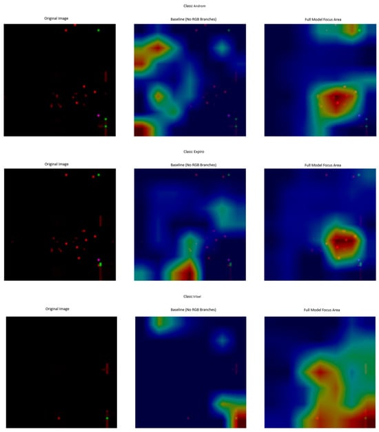
Figure 10.
Gran-CAM comparative samples.
As shown in Figure 11, each square represents a filter trained to detect basic visual primitives. The filters demonstrate a sensitivity to color gradients (e.g., transitions from dark to red), specific color blobs (e.g., solid green or blue areas), and simple textures or edge-like patterns. This indicates that the RGB branch learns to decompose the image into fundamental, color-sensitive features from the very first layer, providing a meaningful basis for the subsequent, more complex feature extraction.
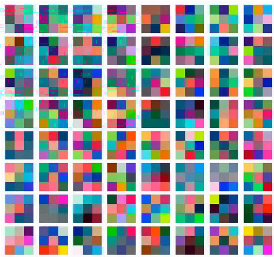
Figure 11.
Visualization of Learned Filters in the First Convolutional Layer of the RGB-Specific Branch.
To further investigate why the RGB-specific branch is so critical to the model’s performance, we visualized the filters learned by its first convolutional layer, as shown in Figure 11. Unlike the complex, multi-channel filters learned by standard backbones, our RGB branch learns a set of fundamental, interpretable features. Many filters specialize in detecting simple color transitions and textures, acting as basic color-sensitive edge or blob detectors. This foundational feature extraction allows the model to build a robust hierarchical representation based on color information, a crucial element that, as our ablation study demonstrates, is indispensable for achieving high accuracy on this task.
5.3. Analysis of Model Complexity Using the PQS-FP (Parameter Quantity Shifting-Fitting Performance) Framework
To rigorously evaluate the relationship between our model’s complexity and its performance, we conducted a systematic analysis using the Parameter Quantity Shifting-Fitting Performance (PQS-FP) coordinate system, as suggested by recent literature [54,55]. This framework provides theoretical insights into a model’s efficiency and scalability by mapping its behavior (under-fitting, good-fitting, over-fitting) based on adjustments in its parameter quantity.
We systematically varied the complexity of our model’s classifier head, creating six distinct configurations with an increasing number of parameters, ranging from a simple single-layer classifier ({128}) to a complex three-layer classifier ({2048, 1024, 512}). Each configuration was trained under identical conditions, and we recorded its total parameter count (P), its best validation loss, and the corresponding training loss. The optimal parameter quantity (P_opt) was defined as the parameter count of the model that achieved the lowest validation loss.
The quantitative results of our experiments are presented in Table 16, and these results are visualized on the PQS-FP coordinate system in Figure 12.
Table 16.
The PQS-FP analysis.
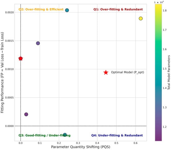
Figure 12.
PQS-FP coordinate system analysis of model complexity.
Together, the table and figure provide a comprehensive view of the model’s behavior, leading to several key insights:
1. Optimal Model Efficiency: As detailed in Table 15, the model with the simplest classifier ({128}) achieved the lowest validation loss (0.0014). This configuration, with 11.26 million parameters, is therefore identified as our optimal model (P_opt). This is a significant finding, highlighted by its position as the origin point (PQS = 0) in Figure 12, demonstrating that our proposed architecture achieves its highest generalization performance in its most parameter-efficient state.
2. Dominance of Over-fitting: The “FP” column in Table 16, calculated as (Validation Loss-Training Loss), shows positive values for almost all configurations. This quantitatively confirms a tendency towards over-fitting. This is visually represented in Figure 12, where all data points are located in the upper half of the PQS-FP plane. The models achieve near-zero training loss, signifying an excellent fit to the training data, but this performance does not fully translate to the unseen validation data.
3. The Impact of Redundant Parameters: Analyzing the data in Table 16 and their positions in Figure 12 reveals that increasing model complexity (i.e., adding more parameters) does not guarantee better performance. As the Parameter Quantity Shifting (PQS) value increases, moving points into the Q1 (Over-fitting and Redundant) quadrant, the validation loss does not consistently decrease. For instance, the model with 18.3 million parameters ({2048, 1024, 512}) has a higher validation loss than the optimal model, confirming that the additional ~7 million parameters are redundant and do not contribute to better generalization.
4. Scalability and Performance Trade-off: The PQS-FP analysis provides a clear view of our model’s scalability. The combined evidence from Table 16 and Figure 12 suggests that while the architecture is robust, adding complexity to the classifier does not scale performance linearly. The optimal point is located at the lower end of the complexity spectrum we tested. This implies that the feature extraction power of the EfficientNet-B0 and DenseNet-121 backbones is highly effective, and a complex classifier is not only unnecessary but can also be detrimental to generalization.
In conclusion, the PQS-FP framework, supported by the detailed results in Table 16 and the visualization in Figure 12, has allowed us to move beyond a single performance metric. We have deeply understood the efficiency, scalability, and fitting behavior of our proposed method. The results strongly support that our model is most effective in a lean, parameter-efficient configuration, which is a desirable characteristic for practical deployment.
6. Discussion
The experimental results demonstrate that our hybrid CNN model achieves superior performance compared to existing malware classification approaches, attaining 98.45% accuracy on the benchmark dataset.
Several limitations warrant discussion. First, while our approach sets a new performance benchmark, the computational requirements exceed simpler methods like Random Forest. Second, the 1.15% accuracy gap between our method and the augmented CycleGAN + CNN approach (99.60%) suggests the potential for improvement through generative data augmentation, albeit at a higher computational cost.
Interestingly, our method achieves this high accuracy without relying on computationally intensive data augmentation techniques, such as those employed by Tekerek and Yapici (2022) [39], whose CycleGAN + CNN model reached 99.60% accuracy but at a significantly higher computational cost. This suggests that our assembly-to-image transformation provides a more efficient and scalable solution for real-world malware detection systems. However, the model does exhibit slightly reduced performance (~94%) on malware families with very few samples (<50), highlighting a limitation in handling rare variants. Future work could explore few-shot learning techniques to address this challenge while maintaining the model’s efficiency and interpretability.
These findings have significant implications for malware detection systems, demonstrating that the assembly-to-image transformation provides a robust representation which outperforms conventional byte-level approaches while maintaining computational feasibility. The results underscore the critical importance of preserving both structural and semantic relationships in malware code for achieving accurate classification. The success of our methodology opens several promising research directions, including the development of hybrid systems that combine our approach’s superior accuracy with the computational efficiency of traditional machine learning methods like Random Forest, particularly for resource-constrained deployment scenarios. Future investigations will focus on: (1) enhancing visualization techniques to bridge the remaining performance gap with computationally intensive augmented methods, (2) integrating attention mechanisms to better capture long-range dependencies in code structure, and (3) extending this approach to other binary analysis tasks where preserving semantic relationships may prove equally beneficial. These advancements could lead to more versatile and efficient malware analysis systems capable of handling increasingly sophisticated threats while maintaining practical deployment characteristics.
7. Limitations
Although the results presented in Table 5, Table 6 and Table 7 highlight leveraging a hybrid CNN architecture’s capability to classify malware families, the model may face limitations due to the inherent complexity and diversity of the malware class set. This is evident in the confusion matrix shown in Figure 7, where certain unique characteristics of specific malware families appear to be insufficiently captured by the pretrained layers, leading to a decline in performance metrics, as discussed in Section 5 with the increasing number of malware classes. While architecture proves effective for classifying the 25 known threats in the MalevisAsm dataset, its robustness may be limited when applied to novel or previously unseen malware variants.
If the model is not trained with enough examples of new threats, its ability to recognize them may be limited. This architecture and similar deep learning models are sensitive to variations in image brightness, scale, or orientation, which can affect generalization. For future work, the model could be further evaluated through additional experiments using external datasets to assess its reproducibility and generalizability across diverse real-world scenarios. Moreover, since the current model may have limitations in adapting to and accurately classifying novel or unseen threats, future research should explore strategies to enhance its robustness and resilience against emerging malware variants.
While the MaleVis dataset provides domain-specific insights for malware visualization, the exclusive reliance on this single dataset limits generalizability. The observed class imbalance, though representative of real-world malware distribution, poses challenges for minority class detection. Future work includes: (1) cross-dataset validation with additional malware datasets, (2) implementation of advanced sampling techniques for severe class imbalance, and (3) collection of additional samples for underrepresented classes. Additionally, cross-dataset evaluation planning is being performed for future studies.
While our experimental validation demonstrates superiority over established CNN architectures in malware image classification, future work will include comparison with cutting-edge approaches such as ISONet [55], which employs input spatial over-parameterization for enhanced training stability. Such comparisons will provide deeper insights into the complementary benefits of our dual-backbone feature fusion approach alongside advanced parameterization techniques in cybersecurity applications.
8. Conclusions
The rapid evolution of malware demands innovative detection techniques that can adapt to increasingly sophisticated threats. This study introduces a vision-based deep learning framework that effectively classifies malware by transforming assembly code into RGB images and leveraging a hybrid CNN architecture. By converting Portable Executable (PE) files into structured visual representations, we enable convolutional networks to extract discriminative features from opcode transitions, achieving 98.45% accuracy on the enhanced MalevisAsm dataset. Our approach demonstrates superior performance compared to existing methods, validating the potential of image-based malware analysis as a robust alternative to traditional static and dynamic techniques.
While the addition of the Dumpware10 dataset demonstrates the model’s generalizability beyond MaleVis, we acknowledge that a large-scale benchmark across multiple, diverse malware datasets (e.g., BIG 2015, Malimg) would provide a more comprehensive evaluation. Such an extensive study is planned as a direct follow-up to the current work, aiming to establish the robustness of our architecture in a wider variety of contexts.
The success of this methodology lies in its ability to capture semantic patterns in assembly code while avoiding the computational overhead of dynamic execution. Unlike signature-based systems, our model generalizes obfuscated and polymorphic variants by interpreting malware behavior through spatial representations. However, challenges remain, including dependency on disassembly tools and the need for further optimization in real-time deployment. Future research could explore adversarial training to enhance resilience against evasion techniques and extend this framework to other binary analysis tasks. Ultimately, this work bridges the gap between low-level code analysis and computer vision, offering a scalable and automated solution for next-generation malware detection. Future research directions include evaluation against emerging architectures with novel training paradigms and exploration of synergistic combinations between our feature fusion strategy and advanced parameterization techniques.
Author Contributions
Conceptualization, Methodology, Software, Formal analysis, Writing—original draft, E.E.D.; Project administration, Validation, Supervision, Writing—review and editing, M.A. All authors have read and agreed to the published version of the manuscript.
Funding
This research received no external funding.
Institutional Review Board Statement
Not applicable.
Informed Consent Statement
Not applicable.
Data Availability Statement
The data presented in this study are available on request from the corresponding author. The data are not publicly available due to privacy.
Acknowledgments
The authors extend their sincere appreciation to all contributors who provided valuable insights and support throughout this research.
Conflicts of Interest
The authors declare no conflicts of interest related to this research.
References
- Available online: https://www.av-test.org/en/statistics/malware/ (accessed on 13 March 2025).
- Admass, W.S.; Munaye, Y.Y.; Diro, A.A. Cyber security: State of the art, challenges and future directions. Cyber Secur. Appl. 2024, 2, 100031. [Google Scholar] [CrossRef]
- Ahmed, I.T.; Jamil, N.; Din, M.M.; Hammad, B.T. Binary and Multi-Class Malware Threads Classification. Appl. Sci. 2022, 12, 12528. [Google Scholar] [CrossRef]
- Akhtar, Z. Malware detection and analysis: Challenges and research opportunities. arXiv 2021, arXiv:2101.08429. [Google Scholar]
- Johny, J.A.; Asmitha, K.A.; Vinod, P.; Radhamani, G.; Rehiman, K.R.; Conti, M. Deep learning fusion for effective malware detection: Leveraging visual features. Clust. Comput. 2025, 28, 135. [Google Scholar] [CrossRef]
- Bozkir, A.S.; Tahillioglu, E.; Aydos, M.; Kara, I. Catch them alive: A malware detection approach through memory forensics, manifold learning and computer vision. Comput. Secur. 2021, 103, 102166. [Google Scholar] [CrossRef]
- Catalano, C.; Chezzi, A.; Angelelli, M.; Tommasi, F. Deceiving AI-based malware detection through polymorphic attacks. Comput. Ind. 2022, 143, 103751. [Google Scholar] [CrossRef]
- Divakarla, U.; Reddy, K.H.K.; Chandrasekaran, K. A Novel Approach towards Windows Malware Detection System Using Deep Neural Networks. Procedia Comput. Sci. 2022, 215, 148–157. [Google Scholar] [CrossRef]
- Kumar, S.; Janet, B.; Neelakantan, S. Identification of malware families using stacking of textural features and machine learning. Expert Syst. Appl. 2022, 208, 118073. [Google Scholar] [CrossRef]
- Kara, I. Fileless malware threats: Recent advances, analysis approach through memory forensics and research challenges. Expert Syst. Appl. 2022, 214, 119133. [Google Scholar] [CrossRef]
- Gibert, D.; Mateu, C.; Planes, J.; Marques-Silva, J. Auditing static machine learning anti-Malware tools against metamorphic attacks. Comput. Secur. 2021, 102, 102159. [Google Scholar] [CrossRef]
- Nawaz, M.S.; Fournier-Viger, P.; Nawaz, M.Z.; Chen, G.; Wu, Y. MalSPM: Metamorphic malware behavior analysis and classification using sequential pattern mining. Comput. Secur. 2022, 118, 102741. [Google Scholar] [CrossRef]
- Kuriyal, V.; Bordoloi, D.; Singh, D.P.; Tripathi, V. Metamorphic and polymorphic malware detection and classification using dynamic analysis of API calls. AIP Conf. Proc. 2022, 2481, 020029. [Google Scholar]
- Deng, X.; Mirkovic, J. Polymorphic malware behavior through network trace analysis. In Proceedings of the 2022 14th International Conference on Communication Systems & Networks (COMSNETS), Bangalore, India, 4–8 January 2022; pp. 138–146. [Google Scholar]
- Selamat, N.S.; Ali, F.H.M. Polymorphic Malware Detection based on Supervised Machine Learning. J. Posit. Sch. Psychol. 2022, 6, 8538–8547. [Google Scholar]
- Akhtar, M.S.; Feng, T. Malware Analysis and Detection Using Machine Learning Algorithms. Symmetry 2022, 14, 2304. [Google Scholar] [CrossRef]
- Al-Hashmi, A.A.; Ghaleb, F.A.; Al-Marghilani, A.; Yahya, A.E.; Ebad, S.A.; Saqib, M.; Darem, A.A. Deep-Ensemble and Multifaceted Behavioral Malware Variant Detection Model. IEEE Access 2022, 10, 42762–42777. [Google Scholar] [CrossRef]
- Quebrado, M.; Serra, E.; Cuzzocrea, A. Android Malware Identification and Polymorphic Evolution Via Graph Representation Learning. In Proceedings of the 2021 IEEE International Conference on Big Data (Big Data), Orlando, FL, USA, 15–18 December 2021; pp. 5441–5449. [Google Scholar]
- Chowdhury, I.R.; Bhowmik, D. Capturing Malware Behaviour with Ontology-based Knowledge Graphs. In Proceedings of the 2022 IEEE Conference on Dependable and Secure Computing (DSC), Edinburgh, UK, 22–24 June 2022; pp. 1–7. [Google Scholar]
- Sriram, S.; Vinayakumar, R.; Sowmya, V.; Alazab, M.; Soman, K.P. Multi-scale learning based malware variant detection using spatial pyramid pooling network. In Proceedings of the IEEE INFOCOM 2020 IEEE Conference on Computer Communications Workshops (INFOCOM WKSHPS), Toronto, ON, Canada, 6–9 July 2020; pp. 740–745. [Google Scholar]
- Sern, L.J.; Keng, T.K.; Fu, C.Z. BinImg2Vec: Augmenting Malware Binary Image Classification with Data2Vec. In Proceedings of the 2022 1st International Conference on AI in Cybersecurity (ICAIC), Victoria, TX, USA, 24–26 May 2022; pp. 1–6. [Google Scholar]
- Azeem, M.; Khan, D.; Iftikhar, S.; Bawazeer, S.; Alzahrani, M. Analyzing and comparing the effectiveness of malware detection: A study of machine learning approaches. Heliyon 2024, 10, e23574. [Google Scholar] [CrossRef]
- Sun, G.; Qian, Q. Deep Learning and Visualization for Identifying Malware Families. IEEE Trans. Dependable Secur. Comput. 2021, 18, 283–295. [Google Scholar] [CrossRef]
- Hemalatha, J.; Roseline, S.A.; Geetha, S.; Kadry, S.; Damaševičius, R. An Efficient DenseNet-Based Deep Learning Model for Malware Detection. Entropy 2021, 23, 344. [Google Scholar] [CrossRef]
- Anandhi, V.; Vinod, P.; Menon, V.G. Malware Visualization and Detection Using DenseNets. Pers. Ubiquitous Comput. 2021, 28, 153–169. [Google Scholar] [CrossRef]
- Mai, J.; Cao, C.; Shi, F.; Chen, X. Malware Variant Detection Based on Decomposed Deep Convolutional Network. In Proceedings of the 2021 IEEE 6th International Conference on Big Data Analytics (ICBDA), Xiamen, China, 5–8 March 2021. [Google Scholar]
- de Oliveira, A.S.; Sassi, R.J. Behavioral Malware Detection using Deep Graph Convolutional Neural Networks. Int. J. Comput. Appl. 2021, 174, 1–8. [Google Scholar] [CrossRef]
- Aditya, W.R.; Girinoto; Hadiprakoso, R.B.; Waluyo, A. Deep learning for malware classification platform using windows api call sequence. In Proceedings of the 2021 International Conference on Informatics, Multimedia, Cyber and Information System (ICIMCIS), Jakarta, Indonesia, 28–29 October 2021. [Google Scholar]
- Jeon, J.; Jeong, B.; Baek, S.; Jeong, Y.-S. Hybrid Malware Detection Based on Bi-LSTM and SPP-Net for Smart IoT. IEEE Trans. Ind. Inform. 2021, 18, 4830–4837. [Google Scholar] [CrossRef]
- Baek, S.; Jeon, J.; Jeong, B.; Jeong, Y. Two-Stage Hybrid Malware Detection Using Deep Learning. Hum. Centric Comput. Inf. Sci. 2021, 11, 27. [Google Scholar]
- Nataraj, L.; Karthikeyan, S.; Jacob, G.; Manjunath, B.S. Malware images: Visualization and automatic classification. In Proceedings of the 8th International Symposium on Visualization for Cyber Security, Pittsburgh, PA, USA, 20 July 2011; pp. 1–7. [Google Scholar]
- Bozkir, A.S.; Cankaya, A.O.; Aydos, M. Utilization and comparision of convolutional neural networks in malware recognition. In Proceedings of the 2019 27th Signal Processing and Communications Applications Conference (SIU), Sivas, Turkey, 24–26 April 2019; pp. 1–4. [Google Scholar]
- Jian, Y.; Kuang, H.; Ren, C.; Ma, Z.; Wang, H. A novel framework for image-based malware detection with a deep neural network. Comput. Secur. 2021, 109, 102400. [Google Scholar] [CrossRef]
- Acharya, J.; Chuadhary, A.; Chhabria, A.; Jangale, S. Detecting malware, malicious URLs and virus using machine learning and signature matching. In Proceedings of the 2021 2nd International Conference for Emerging Technology, INCET, Belagavi, India, 21–23 May 2021; pp. 1–5. [Google Scholar]
- Xu, Z.; Fang, X.; Yang, G. Malbert : A novel pre-training method for malware detection. Comput. Secur. 2021, 111, 102458. [Google Scholar] [CrossRef]
- Available online: https://umap-learn.readthedocs.io/en/latest/ (accessed on 13 March 2025).
- Deng, H.; Guo, C.; Shen, G.; Cui, Y.; Ping, Y. MCTVD: A malware classification method based on three-channel visualization and deep learning. Comput. Secur. 2023, 126, 103084. [Google Scholar] [CrossRef]
- Xiang, Q.; Wang, X.; Lei, L.; Song, Y. Dynamic bound adaptive gradient methods with belief in observed gradients. Pattern Recognit. 2025, 168, 111819. [Google Scholar] [CrossRef]
- Tekerek, A.; Yapici, M.M. A novel malware classification and augmentation model based on convolutional neural network. Comput. Secur. 2022, 112, 102515. [Google Scholar] [CrossRef]
- Salas, M.P.; de Geus, P.L. Deep learning applied to imbalanced malware datasets classification. J. Internet Serv. Appl. 2024, 15, 342–359. [Google Scholar] [CrossRef]
- Naeem, H.; Guo, B.; Naeem, M.R.; Ullah, F.; Aldabbas, H.; Javed, M.S. Identification of malicious code variants based on image visualization. Comput. Electr. Eng. 2019, 76, 225–237. [Google Scholar] [CrossRef]
- Drew, J.; Moore, T.; Hahsler, M. Polymorphic malware detection using sequence classification methods. In Proceedings of the 2016 IEEE Security and Privacy Workshops (SPW), San Jose, CA, USA, 22–26 May 2016; pp. 81–87. [Google Scholar]
- Narayanan, B.N.; Djaneye-Boundjou, O.; Kebede, T.M. Performance analysis of machine learning and pattern recognition algorithms for malware classification. In Proceedings of the 2016 IEEE National Aerospace and Electronics Conference (NAECON) and Ohio Innovation Summit (OIS), Dayton, OH, USA, 25–29 July 2016; pp. 338–342. [Google Scholar]
- Hassen, M.; Chan, P.K. Scalable function call graph-based malware classification. In Proceedings of the Seventh ACM on Conference on Data and Application Security and Privacy, Scottsdale, AZ, USA, 22–24 March 2017; pp. 239–248. [Google Scholar]
- Lin, W.C.; Yeh, Y.R. Efficient malware classification by binary sequences with one-dimensional convolutional neural networks. Mathematics 2022, 10, 608. [Google Scholar] [CrossRef]
- Gibert, D.; Mateu, C.; Planes, J.; Vicens, R. Classification of malware by using structural entropy on convolutional neural networks. In Proceedings of the AAAI Conference on Artificial Intelligence, New Orleans, LA, USA, 2–7 February 2018; Volume 32. [Google Scholar]
- Ding, Y.; Wang, S.; Xing, J.; Zhang, X.; Qi, Z.; Fu, G.; Zhang, J. Malware classification on imbalanced data through self-attention. In Proceedings of the 2020 IEEE 19th International Conference on Trust, Security and Privacy in Computing and Communications (TrustCom), Guangzhou, China, 29 December 2020–1 January 2021; pp. 154–161. [Google Scholar]
- Gibert, D.; Mateu, C.; Planes, J. An end-to-end deep learning architecture for classification of malware’s binary content. In International Conference on Artificial Neural Networks; Springer International Publishing: Berlin/Heidelberg, Germany, 2018; pp. 383–391. [Google Scholar]
- Kim, J.Y.; Bu, S.J.; Cho, S.B. Malware detection using deep transferred generative adversarial networks. In Proceedings of the Neural Information Processing: 24th International Conference, ICONIP 2017, Guangzhou, China, 14–18 November 2017; Proceedings, Part I 24 (pp. 556–564). Springer International Publishing: Cham, Switzerland, 2017. [Google Scholar]
- Kim, J.Y.; Cho, S.B. Obfuscated malware detection using deep generative model based on global/local features. Comput. Secur. 2022, 112, 102501. [Google Scholar] [CrossRef]
- Gibert, D.; Mateu, C.; Planes, J.; Vicens, R. Using convolutional neural networks for classification of malware represented as images. J. Comput. Virol. Hacking Tech. 2019, 15, 15–28. [Google Scholar] [CrossRef]
- Ren, Z.; Chen, G.; Lu, W. Malware visualization methods based on deep convolution neural networks. Multimed. Tools Appl. 2020, 79, 10975–10993. [Google Scholar] [CrossRef]
- Selvaraju, R.R.; Cogswell, M.; Das, A.; Vedantam, R.; Parikh, D.; Batra, D. Grad-cam: Visual explanations from deep networks via gradient-based localization. arXiv 2016, arXiv:1610.02391. [Google Scholar]
- Xiang, Q.; Wang, X.; Lai, J.; Lei, L.; Song, Y.; He, J.; Li, R. Quadruplet depth-wise separable fusion convolution neural network for ballistic target recognition with limited samples. Expert Syst. Appl. 2024, 235, 121182. [Google Scholar] [CrossRef]
- Xiang, Q.; Wang, X.; Song, Y.; Lei, L. ISONet: Reforming 1DCNN for aero-engine system inter-shaft bearing fault diagnosis via input spatial over-parameterization. Expert Syst. Appl. 2025, 277, 127248. [Google Scholar] [CrossRef]
Disclaimer/Publisher’s Note: The statements, opinions and data contained in all publications are solely those of the individual author(s) and contributor(s) and not of MDPI and/or the editor(s). MDPI and/or the editor(s) disclaim responsibility for any injury to people or property resulting from any ideas, methods, instructions or products referred to in the content. |
© 2025 by the authors. Licensee MDPI, Basel, Switzerland. This article is an open access article distributed under the terms and conditions of the Creative Commons Attribution (CC BY) license (https://creativecommons.org/licenses/by/4.0/).