

Pore Pressure Prediction and Fluid Contact Determination: A Case Study of the Cretaceous Sediments in the Bredasdorp Basin, South Africa


Abstract
1. Introduction
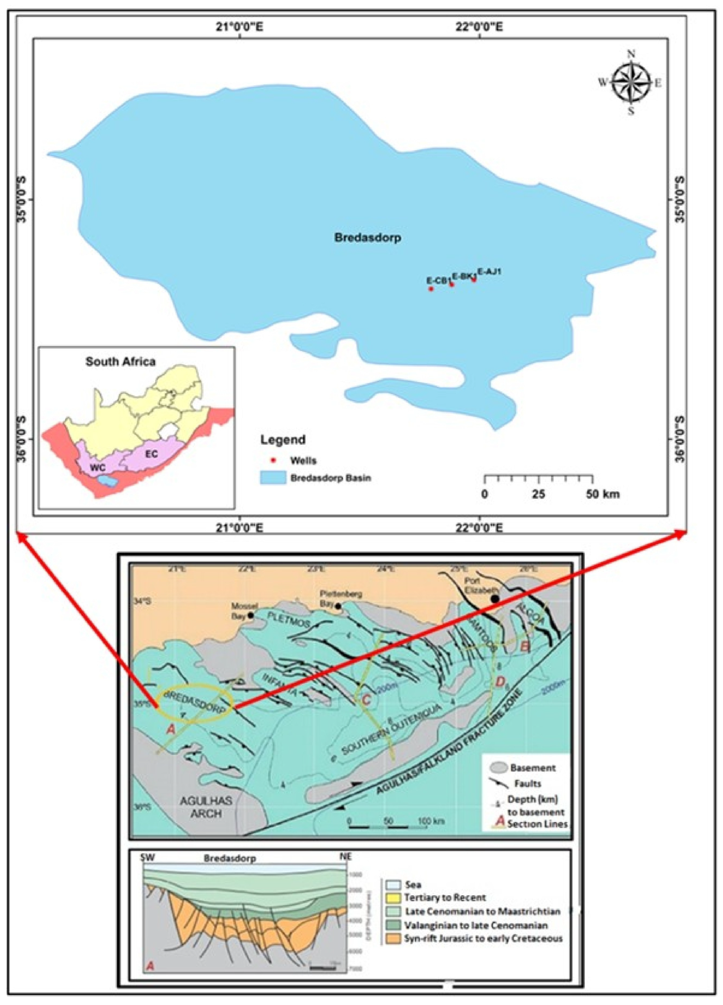
2. Location of the Study Area and the Geological Background
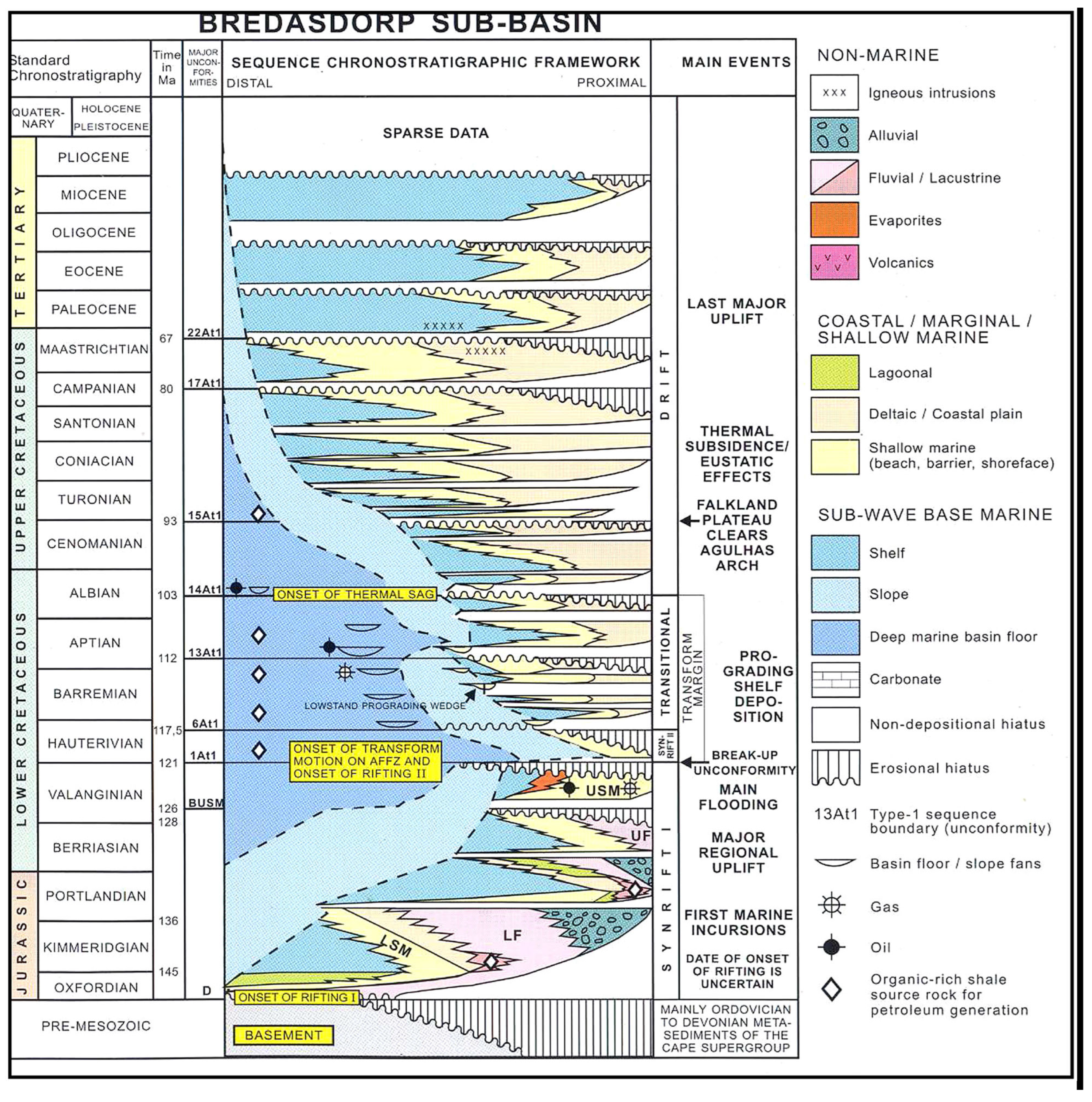
- Tectonic history of the Bredasdorp Basin
- Syn-rift Phase
- Transition Phase
- Drift Phase
3. Materials and Methods
3.1. Pore Pressure Prediction Methods
3.1.1. Ben Eaton’s Resistivity Method with Depth-Dependent Normal Compaction Trend (NCT) Line
- = pore pressure gradient;
- = overburden stress gradient (ppg), (psi/ft);
- = hydrostatic pore pressure gradient, normally 0.45 psi/ft/1.03 MPa/km based on the water salinity of the region;
- = observed shale resistivity (ohm/m);
- = normal shale resistivity (hydrostatic pressure).
- = shale resistivity in the normal compaction condition;
- = shale resistivity in a mudline;
- = constant number;
- = profundity of mud line below.
- = shale resistivity measured at depth ;
- = logarithmic resistivity normal compaction line slope;
- = mudline normal compaction shale resistivity.
3.1.2. Ben Eaton’s Sonic Velocity Method with Depth-Dependent Normal Compaction Trend (NCT) Line
- = sonic transit travel time/the slowness in shale at normal pressure (μs/ft).
- = seismic velocity at depth Z;
- = ground surface velocity;
- = a constant.
- = (µs/m);
- Z = the depth in meters.
- = compressional transit time in the porosity-free shale matrix;
- = mudline transit time;
- = is the constant.
3.1.3. Application of Eaton’s Method by Developing Normal Compaction Trend (NCT) in Resistivity and Sonic Velocity Log Plots
3.2. Different Pore Pressure Prediction Methods
3.2.1. Mathews and Kelly Method
- = break inclination at the purpose of investment (psi/ft);
- = formation pressure (psi);
- = depth of interest (ft);
- = matrix stress (psi);
- = matrix stress coefficient;
- = depth at normal matrix.
3.2.2. Bowers Method
- = Velocity (Ft/s);
- = Effective pressure (Psi);
- = Maximum effective pressure (Psi);
- and = Bowers empirical coefficients.
3.2.3. Barker and Wood Method
- = True Vertical Depth Below Mud Line
3.2.4. Ben Eaton Modified
- = pore pressure (psi);
- = overburden;
- = fracture gradient (psi/ft);
- = Depth (ft);
- v = Poisson ratio.
3.3. Fluid Contacts Determination
4. Results
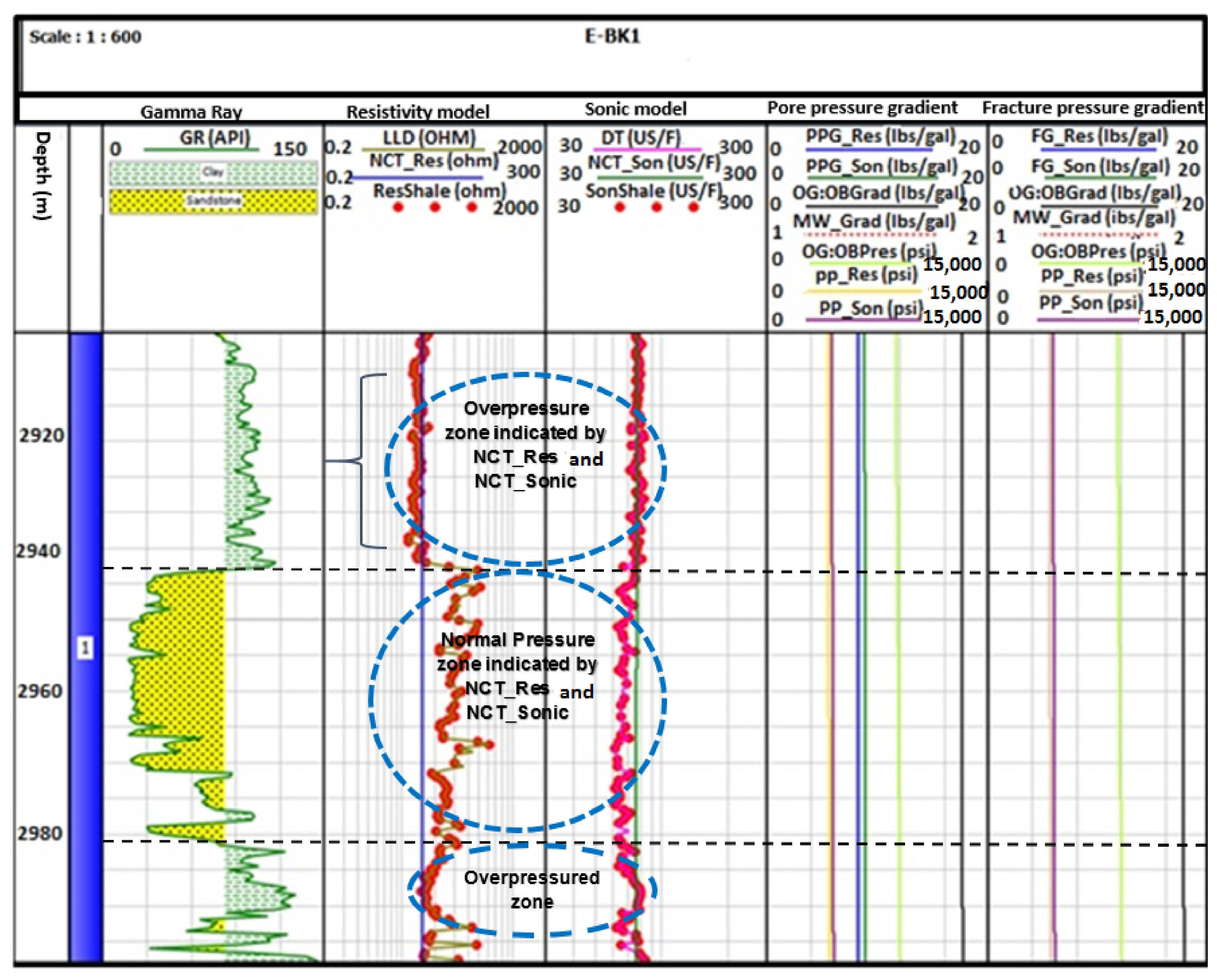
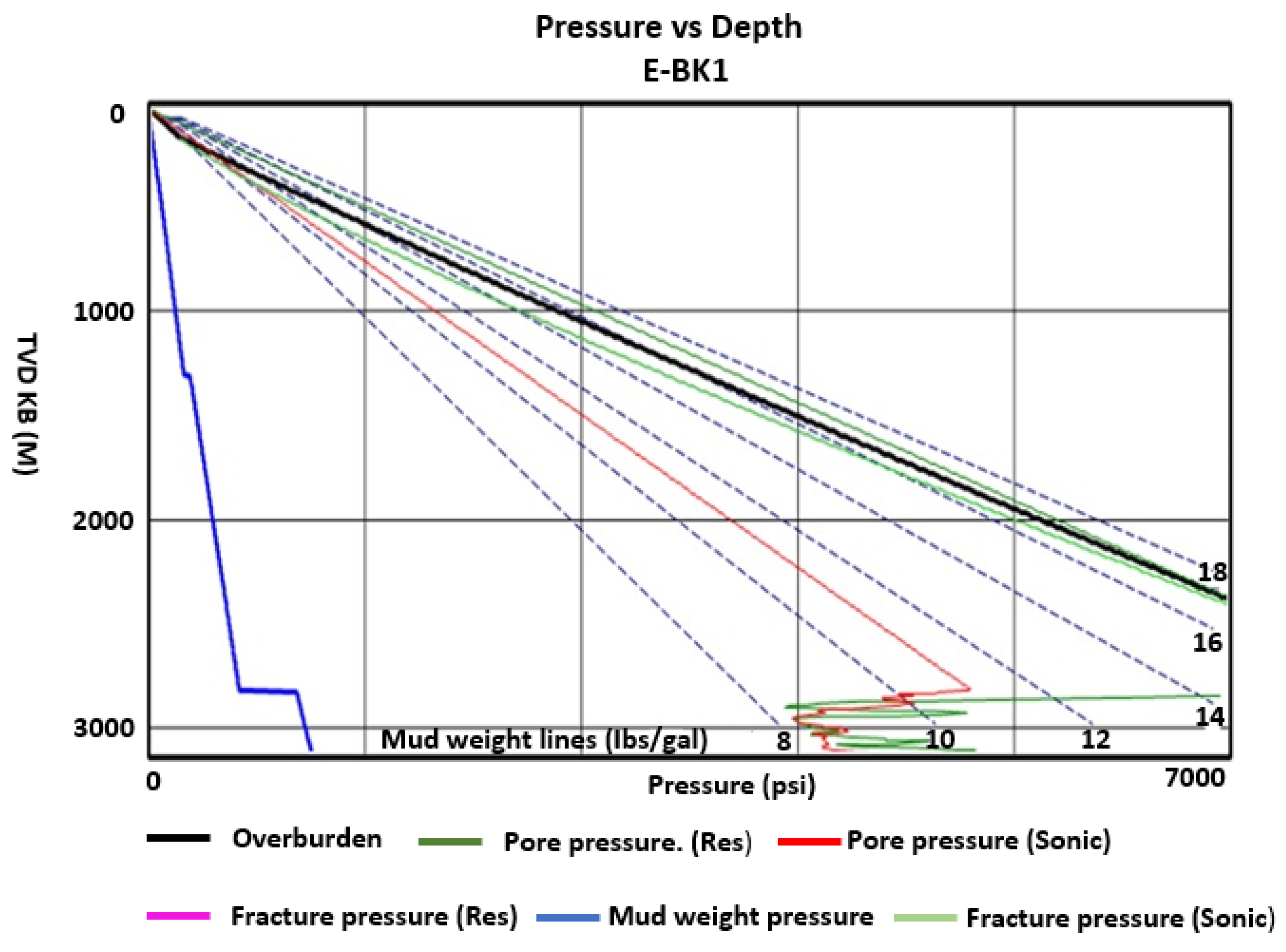
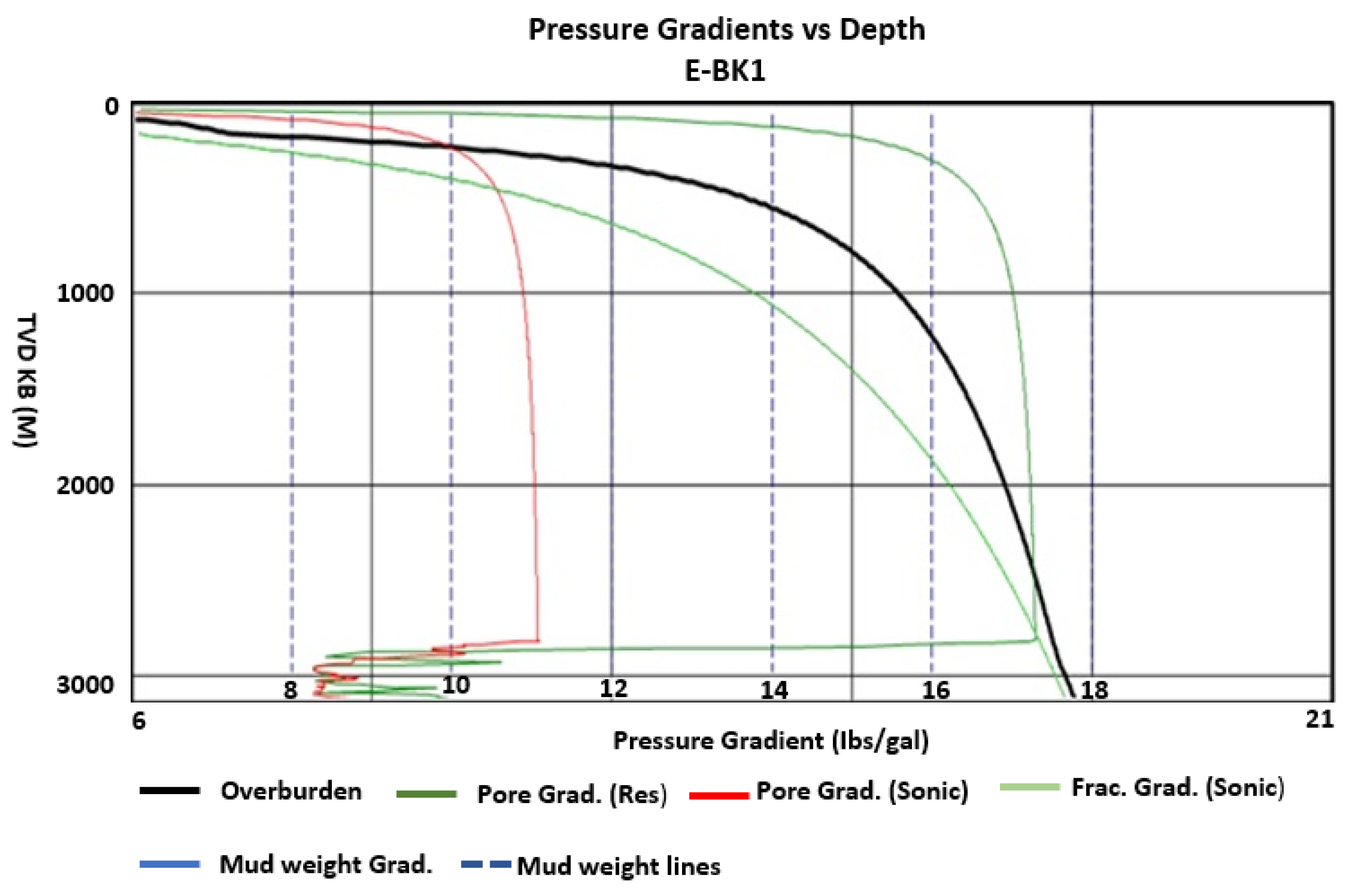
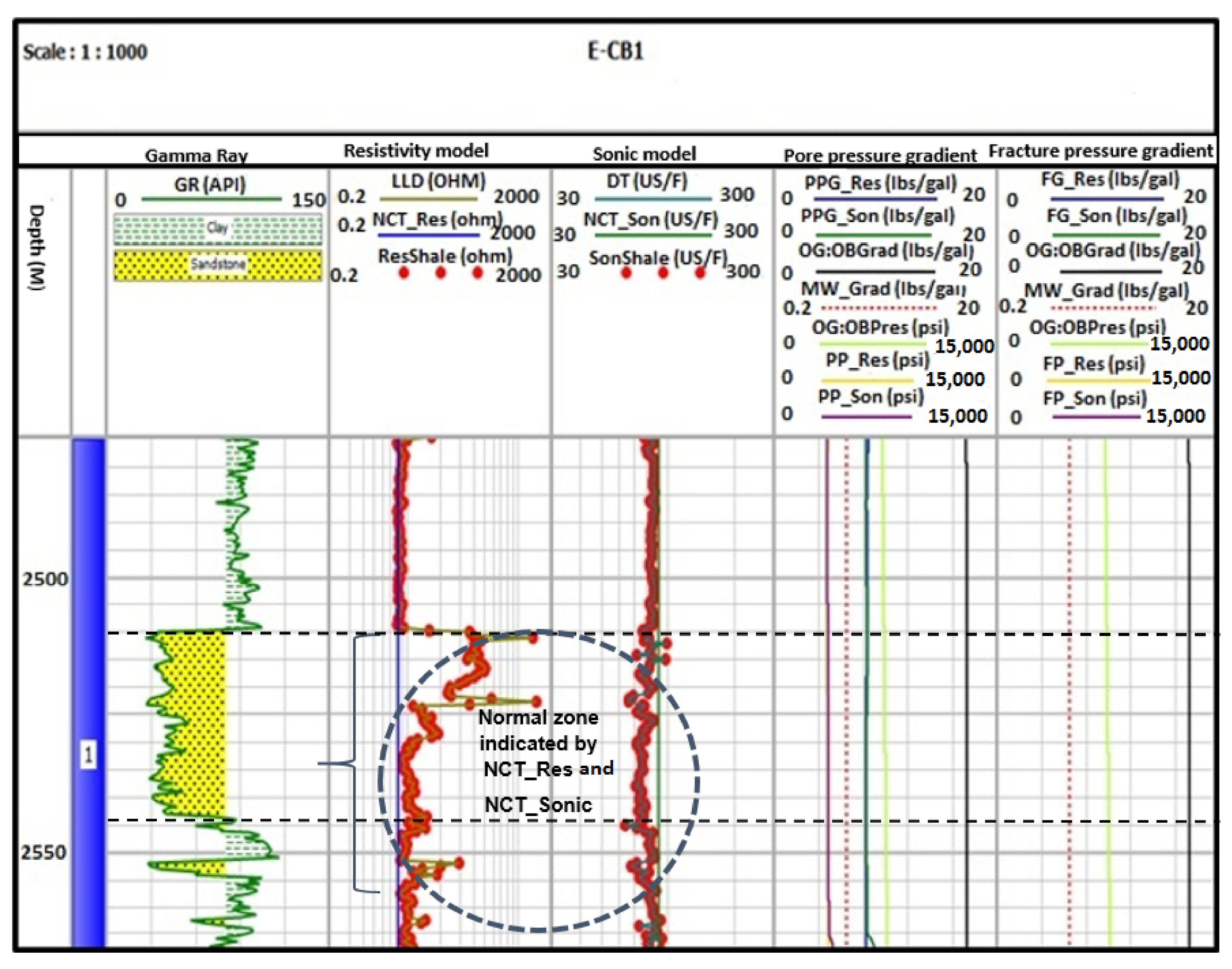
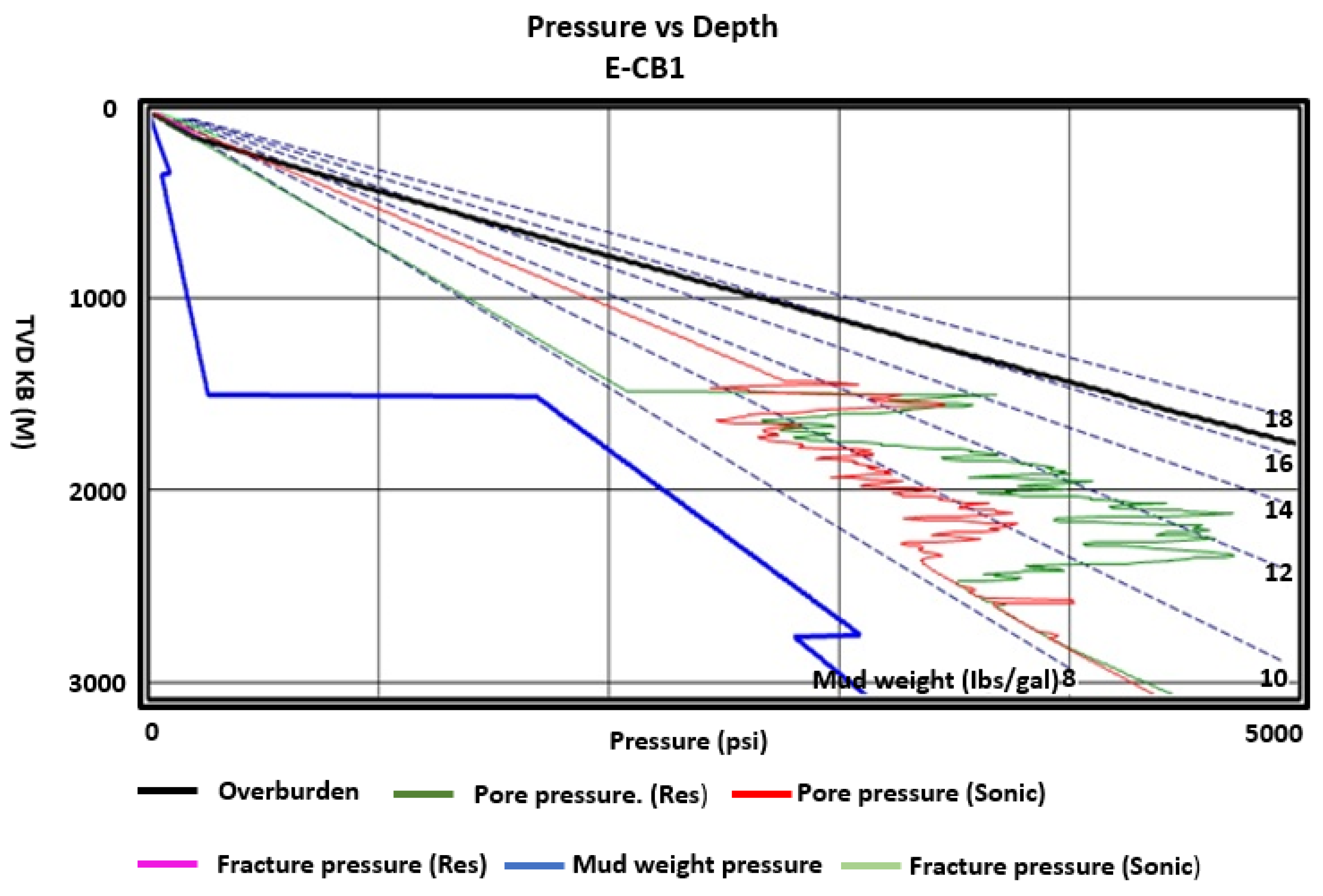
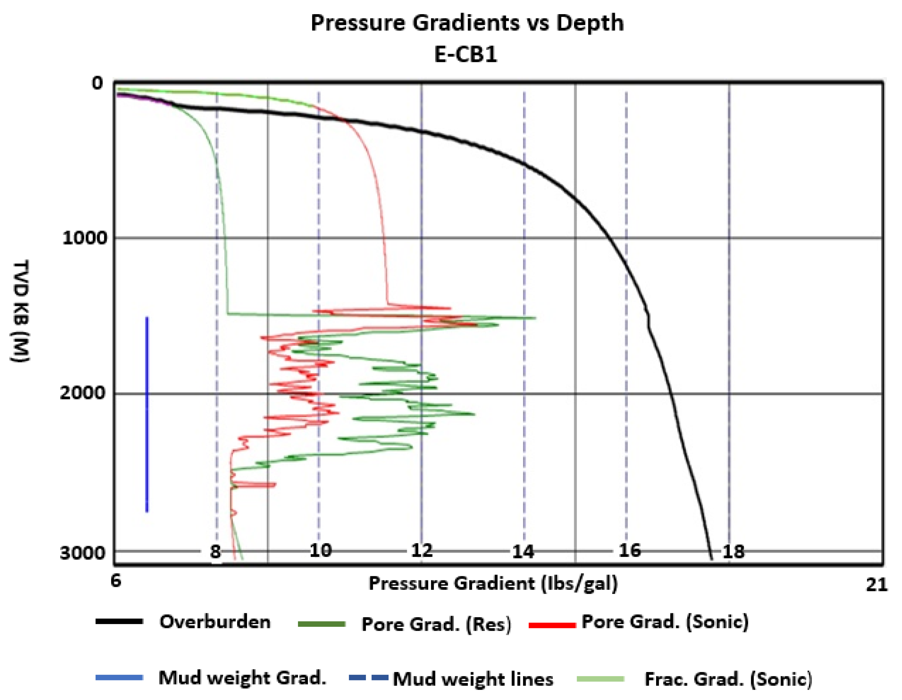
4.1. Pore Pressure Prediction from Resistivity and Sonic Logs
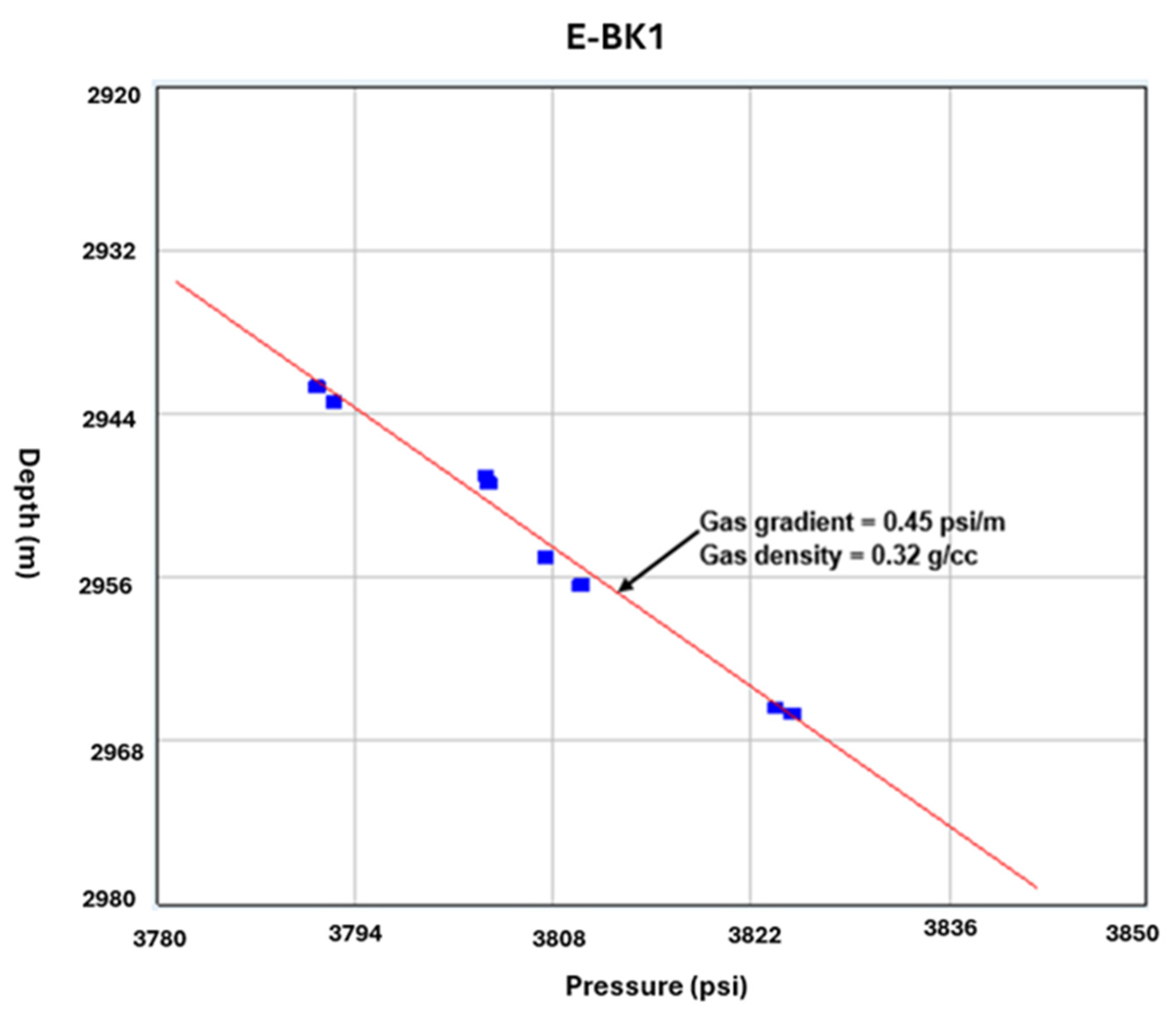
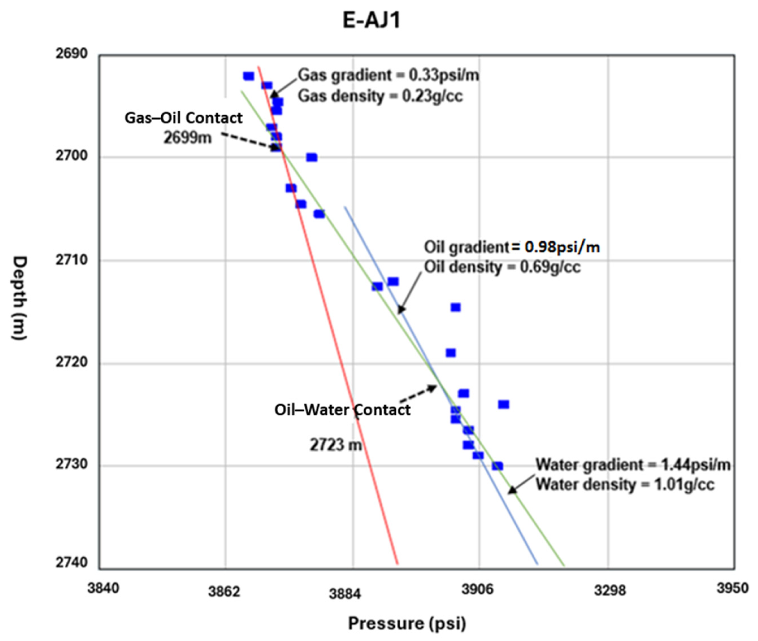
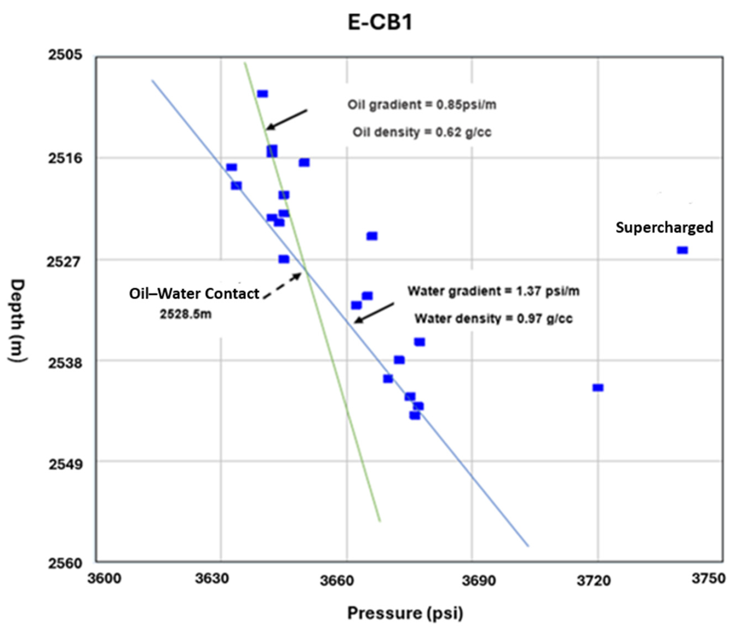
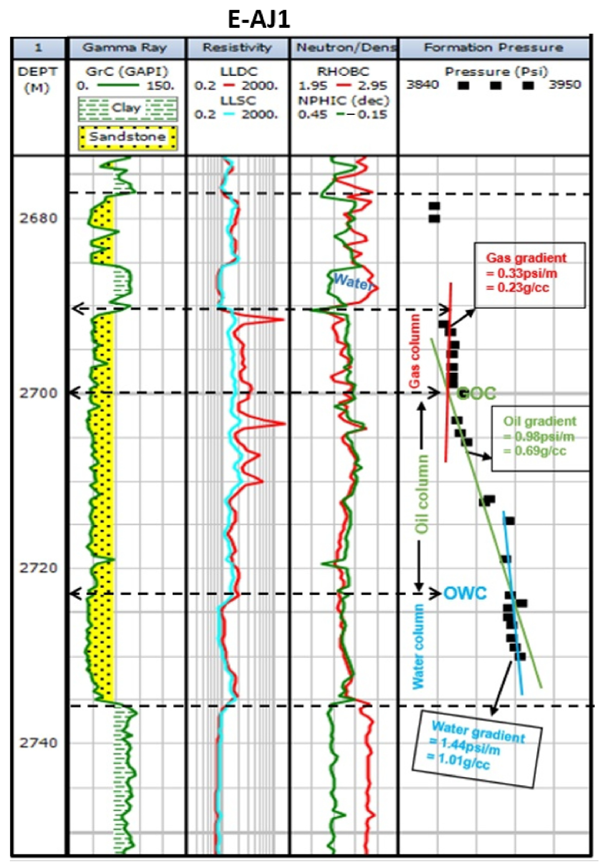
4.2. Fluid Contacts Determination Using Repeat Formation Test (RFT) Data
4.3. Log and RFT Data Fluid Contacts Comparison
5. Discussion
6. Conclusions
Author Contributions
Funding
Institutional Review Board Statement
Informed Consent Statement
Data Availability Statement
Acknowledgments
Conflicts of Interest
References
- Acho, C.B. Assessing Hydrocarbon Potential in Cretaceous Sediments in the Western Bredasdorp Sub-Basin in the Outeniqua Basin South Africa. Master’s Thesis, University of the Western Cape, Cape Town, South Africa, 2015. [Google Scholar]
- Baiyegunhi, T.L.; Liu, K.; Gwavava, O.; Wagner, N.; Baiyegunhi, C. Geochemical evaluation of the cretaceous mudrocks and sandstones (Wackes) in the Southern Bredasdorp Basin, Offshore South Africa: Implications for hydrocarbon potential. Minerals 2020, 10, 595. [Google Scholar] [CrossRef]
- Magoba, M.; Opuwari, M.; Liu, K. The effect of diagenetic minerals on the petrophysical properties of sandstone reservoir: A case study of the upper shallow marine sandstones in the central Bredasdorp basin, offshore South Africa. Minerals 2024, 14, 396. [Google Scholar] [CrossRef]
- Radwan, A.E. Modeling pore pressure and fracture pressure using integrated well logging, drilling based interpretations and reservoir data in the Giant El Morgan oil Field, Gulf of Suez, Egypt. J. Afr. Earth Sci. 2021, 178, 104165. [Google Scholar] [CrossRef]
- Uchechukwu, E.E. Pore Pressure Prediction: A Case Study of Sandstone Reservoirs, Bredasdorp Basin, South Africa. Master’s Thesis, University of the Western Cape, Cape Town, South Africa, 2014. [Google Scholar]
- Tang, H.; Luo, J.; Qiu, K.; Chen, Y.; Tan, C.P. Worldwide pore pressure prediction: Case studies and methods. In Proceedings of the SPE Asia Pacific Oil and Gas Conference and Exhibition, Jakarta, Indonesia, 20–22 September 2011; pp. 140–954. [Google Scholar]
- Drews, M.C.; Shatyrbayeva, I.; Bohnsack, D.; Duschl, F.; Obermeier, P.; Loewer, M.; Flechtner, F.; Keim, M. The role of pore pressure and its prediction in deep geothermal energy drilling–examples from the North Alpine Foreland Basin, SE Germany. Pet. Geosci. 2022, 28, 2021–2061. [Google Scholar] [CrossRef]
- Ayodele, O.L.; van Bever Donker, J.M.; Opuwari, M. Pore pressure prediction of some selected wells from the Southern Pletmos Basin, offshore South Africa. S. Afr. J. Geol. 2016, 119, 203–214. [Google Scholar] [CrossRef]
- United Nations. The Sustainable Development Goals Report. 2022. Available online: https://unstats.un.org/sdgs/report/2022/The-Sustainable-Development-Goals-Report-2022.pdf (accessed on 28 August 2024).
- Ichenwo, J.L.; Olatunji, A. Pore pressure and fracture pressure forecast in Niger Delta. Int. J. Eng. Res. Technol. 2018, 7, 338–344. [Google Scholar]
- Zhang, Y.; Lv, D.; Wang, Y.; Liu, H.; Song, G.; Gao, J. Geological characteristics and abnormal pore pressure prediction in shale oil formations of the Dongying depression, China. Energy Sci. Eng. 2020, 8, 1962–1979. [Google Scholar] [CrossRef]
- Ashena, R.; Ghorbani, F.; Mubashir, M. The root cause analysis of an oilwell blowout and explosion in the Middle East. J. Pet. Eng. 2021, 207, 109–134. [Google Scholar] [CrossRef]
- Dutta, N.C.; Bachrach, R.; Mukerji, T. Quantitative Analysis of Geopressure for Geoscientists and Engineers; Cambridge University Press: Cambridge, UK, 2021. [Google Scholar]
- Asfha, D.T.; Gebretsadik, H.T.; Latiff, A.H.A.; Rahmani, O. Predictive pore pressure modeling using well-log data in the West Baram Delta, offshore Sarawak Basin, Malaysia. Geomech. Geophys. Geo-Energy Geo-Resour. 2024, 10, 196. [Google Scholar] [CrossRef]
- Azadpour, M.; Manaman, N.S.; Kadkhodaie-Ilkhchi, A.; Sedghipour, M.R. Pore pressure prediction and modeling using well-logging data in one of the gas fields in south of Iran. J. Pet. Sci. Eng. 2015, 128, 15–23. [Google Scholar] [CrossRef]
- Tawfeeq, Y.J.; Al-Mufarji, M.A.; Aziz, Q.A.A. Predicating of Formation Pore Pressures in Tertiary Reservoirs Using Geophysical Wireline Log Data. Iraqi Geol. J. 2024, 57, 78–91. [Google Scholar] [CrossRef]
- Ejeh, C.J.; Anumah, P.; Woherem, C.E.; Olalekan, A.; Manjum, D.E. Effect of hydrodynamic tilting at fluid contacts to reservoir production performance. Results Eng. 2020, 8, 100184. [Google Scholar] [CrossRef]
- Niculescu, B.M.; Ciupercă, C.L. Identification of fluid contacts by using formation pressure data and geophysical well logs. In Proceedings of the 19th International Multidisciplinary Scientific GeoConference, Albena, Bulgaria, 30 June–6 July 2019; pp. 897–908. [Google Scholar]
- Opuwari, M. An integrated approach of fluid contact determination of the Albian age sandstone reservoirs of the Orange Basin Offshore South Africa. Mar. Georesources Geotechnol. 2020, 39, 876–888. [Google Scholar] [CrossRef]
- Vail, P.R. Seismic stratigraphy and global changes of sea level. Mem. Am. Assoc. Pet. Geol. 1977, 26, 49–50. [Google Scholar]
- Ogbamikhumi, A.; Akanzua-Adamczyk, A.H.; Ahiwe, L. Pressure analysis and fluid contact prediction for alpha reservoir (a partially appraised field) onshore niger delta. Niger. J. Technol. 2017, 36, 801–805. [Google Scholar] [CrossRef]
- Ehsan, M.; Manzoor, U.; Chen, R.; Hussain, M.; Abdelrahman, K.; Radwan, A.E.; Ullah, J.; Iftikhar, M.K.; Arshad, F. Pore pressure prediction based on conventional well logs and seismic data using an advanced machine learning approach. J. Rock Mech. Geotech. Eng. 2025, 17, 2727–2740. [Google Scholar] [CrossRef]
- Osarogiagbon, A.U.; Oloruntobi, O.; Khan, F.; Venkatesan, R.; Gillard, P. Combining porosity and resistivity logs for pore pressure prediction. J. Pet. Sci. Eng. 2021, 205, 108819. [Google Scholar] [CrossRef]
- Alabere, A.O.; Akangbe, O.K. Pore pressure prediction in Niger Delta high pressure, high temperature (HP/HT) domains using well logs and 3D seismic data: A case study of X-field, onshore Niger Delta. J. Pet. Explor. Prod. Technol. 2021, 11, 3747–3758. [Google Scholar] [CrossRef]
- Farsi, M.; Mohamadian, N.; Ghorbani, H.; Wood, D.A.; Davoodi, S.; Moghadasi, J.; Ahmadi Alvar, M. Predicting formation pore-pressure from well-log data with hybrid machine-learning optimization algorithms. Nat. Resour. Res. 2021, 30, 3455–3481. [Google Scholar] [CrossRef]
- Abass, A.E.; Teama, M.A.; Kassab, M.A.; Elnaggar, A.A. Integration of mud logging and wireline logging to detect overpressure zones: A case study of middle Miocene Kareem Formation in Ashrafi oil field, Gulf of Suez, Egypt. J. Pet. Explor. Prod. Technol. 2020, 10, 515–535. [Google Scholar] [CrossRef]
- Blinov, V.; Weinheber, P.; Vasilyev, D.; Ivashin, M.; Shtun, S.; Samoylenko, A.; Ganichev, D.; Tereschuk, A.; Alexeev, I. Contact Determination, Fluid Typing and Deliverability Estimation in North Caspian Appraisal Wells. In Proceedings of the SPE Russian Petroleum Technology Conference, Moscow, Russia, 26–28 October 2015; p. SPE-176598. [Google Scholar] [CrossRef]
- Proett, M.A.; Chin, W.C.; Manohar, M.; Sigal, R.; Wu, J. Multiple factors that influence wireline formation tester pressure measurements and fluid contacts estimates. In Proceedings of the SPE Annual Technical Conference and Exhibition? New Orleans, LA, USA, 30 September–3 October 2001; p. SPE-71566. [Google Scholar] [CrossRef]
- Petroleum Exploration in South Africa: Information and Opportunities Brochure; Brochures–Petroleum Agency SA: Cape Town, South Africa, 2012; Available online: https://www.petroleumagencysa.com/brochures/ (accessed on 11 March 2024).
- Van Bloemenstein, C.B. Petrographic Characterization of Sandstones in Borehole E-BA1, Block 9, Bredasdorp Basin, Offshore South Africa. Ph.D. Thesis, University of the Western Cape, Cape Town, South Africa, 2006. [Google Scholar]
- Hussien, T.M.H. Formation Evaluation of Deep-Water Reservoirs in the 13A and 14A Sequences of the Central Bredasdorp Basin, Offshore South Africa. Master’s Thesis, University of the Western Cape, Cape Town, South Africa, 2014. [Google Scholar]
- Magoba, M. Petrophysical Evaluation of Sandstone Reservoir of Well E-AH1, E-BW1 and E-L1 Central Bredasdorp Basin, Offshore South Africa, Offshore South Africa. Master’s Thesis, University of the Western Cape, Cape Town, South Africa, 2014. [Google Scholar]
- Turner, J.R.; Grobbler, N.; Sontundu, S. Geological modelling of the Aptian and Albian sequences within Block 9, the Bredasdorp basin, Offshore South Africa. Afr. J. Sci. 2000, 31, 80. [Google Scholar]
- Opuwari, M.; Dominick, N. Sandstone reservoir zonation of the North-Western Bredasdorp Basin South Africa using core data. J. Appl. Geophys. 2021, 193, 104–425. [Google Scholar] [CrossRef]
- Tinker, J.; de Wit, M.; Brown, R. Linking source and sink: Evaluating the balance between onshore erosion and offshore sediment accumulation since Gondwana break-up, South Africa. Tectonophysics 2008, 455, 94–103. [Google Scholar] [CrossRef]
- McMillan, I.K.; Brink, G.I.; Broad, D.S.; Maier, J.J. Late Mesozoic sedimentary basins off the south coast of South Africa. In Sedimentary Basins of the World; Elsevier: Amsterdam, The Netherlands, 1997; Volume 3, pp. 319–376. [Google Scholar] [CrossRef]
- Davies, C.P. Unusual biomarker maturation ratio changes through the oil window, a consequence of varied thermal history. Org. Geochem. 1997, 27, 537–560. [Google Scholar] [CrossRef]
- Storey, B.C.; Curtis, M.L.; Ferris, J.K.; Hunter, M.A.; Livermore, R.A. Reconstruction and break-out model for the Falkland Islands within Gondwana. J. Afr. Earth Sci. 1999, 29, 153–163. [Google Scholar] [CrossRef]
- Schalkwyk, H.J.M. Assessment Controls on Reservoir Performance and the Effects of Granulation Seam Mechanics in the Bredasdorp Basin, South Africa. Ph.D. Thesis, University of the Western Cape, Cape Town, South Africa, 2006. [Google Scholar]
- Van Rensburg, T. Identification of the Physical Controls on the Deposition of Aptian and Albian Deep Water Sands in the Bredasdorp Basin, South Africa. Master’s Thesis, University of Cape Town, Cape Town, South Africa, 2016. [Google Scholar]
- Petroleum Exploration Information and Opportunities: Petroleum Agency, South Africa Brochure. 2003. Available online: https://www.petroleumagencysa.com/images/pdfs/Pet_expl_opp_broch_2017bw1.pdf (accessed on 20 July 2022).
- Opuwari, M.; Afolayan, B.; Mohammed, S.; Amaechi, P.O.; Bareja, Y.; Chatterjee, T. Petrophysical core-based zonation of OW oilfield in the Bredasdorp Basin South Africa. Sci. Rep. 2022, 12, 510. [Google Scholar] [CrossRef]
- Fadipe, O.A. Facies, Depositional Environments and Reservoir Properties of the Albian Age Gas Bearing Sandstone of the Ibhubesi Oil Field, Orange Basin, South Africa. Ph.D. Thesis, University of the Western Cape, Cape Town, South Africa, 2009. [Google Scholar]
- Burden, P.L. Soekor, partners explore possibilities in Bredasdorp Basin off South Africa. Oil Gas J. United States 1992, 90, 109. [Google Scholar]
- Jikelo, N.A. The natural gas resources of southern Africa. J. Afr. Earth Sci. 2000, 31, 34. [Google Scholar]
- Jungslager, E.H.A. Geological Evaluation of the Remaining Prospectivity for Oil and Gas of the Pre-1At1 “Synrift” Succession in Block 9, Republic of South Africa; Unpublished Soekor Techical Report; 1996; SOE-EXP-RPT-0380. [Google Scholar]
- Opuwari, M.; Magoba, M.; Dominick, N.; Waldmann, N. Delineation of Sandstone Reservoir Flow Zones in the Central Bredasdorp Basin, South Africa, Using Core Samples. Nat. Resour. Res. 2021, 30, 3385–3406. [Google Scholar] [CrossRef]
- Broad, D.S.; Jungslager, E.H.A.; McLachlan, I.R.; Roux, J. Offshore Mesozoic basins. S. Afr. J. Geol. 2012, 534–564. [Google Scholar] [CrossRef]
- Yoshida, C.; Ikeda, S.; Eaton, B.A. An investigative study of recent technologies used for prediction, detection, and evaluation of abnormal formation pressure and fracture pressure in North and South America. In Proceedings of the IADC/SPE Asia Pacific Drilling Technology Conference and Exhibition, North and South America, Kuala Lumpur, Malaysia, 9 September 1996. [Google Scholar]
- Lasisi, A.O. Pore Pressure Prediction and Direct Hydrocarbon Indicator: Insight from the Southern Pletmos Basin, Offshore South Africa. Ph.D. Thesis, University of the Western Cape, Cape Town, South Africa, 2014. [Google Scholar]
- Eaton, B.A. The equation for geopressure prediction from well logs. In Proceedings of the SPE Annual Technical Conference and Exhibition, Dallas, TX, USA, 28 September 1975; p. SPE-5544. [Google Scholar]
- Sayers, C.M.; Johnson, G.M.; Denyer, G. Predrill pore-pressure prediction using seismic data. Geophysics 2002, 67, 1286–1292. [Google Scholar] [CrossRef]
- Slotnick, M.M. On seismic computation with applications. Geophysics 1936, 1, 9–22. [Google Scholar] [CrossRef]
- Van Ruth, P.; Hillis, R. Estimating pore pressure in the Cooper Basin, South Australia: Sonic log method in an uplifted basin. Explor. Geophys. 2000, 31, 441–447. [Google Scholar] [CrossRef]
- Tingay, M.R.P.; Hillis, R.R.; Swarbrick, R.E.; Morley, C.K.; Damit, A.R. Origin of overpressure and pore-pressure prediction in the Baram province, Brunei. AAPG Bull. 2009, 93, 51–74. [Google Scholar] [CrossRef]
- Matthews, M.D. Uncertainty-shale pore pressure from borehole resistivity. In Proceedings of the ARMA North America Rock Mechanics Symposium Conference, Houston, TX, USA, 5–10 June 2004. [Google Scholar]
- Zhang, J. Pore pressure Prediction from Well logs: Methods, Modification, and New Approaches. Earth Sci. Rev. 2011, 108, 50–63. [Google Scholar] [CrossRef]
- Bateman, R. Open-Hole Log Analysis and Formation Evaluation; International Human Resources Development Corporation, University of California: Boston, MA, USA, 1985. [Google Scholar]
- Mathews, W.R.; Kelly, J. How to prepare formation pressure and fracture gradient. Oil Gas J. 1967, 20, 92–106. [Google Scholar]
- de Castro, T.M.; Lupinacci, W.M. Comparison between conventional and NMR approaches for formation evaluation of presalt interval in the Buzios Field, Santos Basin, Brazil. J. Pet. Sci. Eng. 2022, 208, 109–679. [Google Scholar] [CrossRef]
- Hossain, S.; Rahman, N. An integrated petrophysical and rock physics characterization of the Mangahewa Formation in the Pohokura field, Taranaki Basin. Sci. Rep. 2025, 15, 4983. [Google Scholar] [CrossRef]
- Wu, P.; Zhao, X.; Ling, H.; Feng, M.; Dong, X.; Gan, C.; Deng, R. Simulation of gas-water identification in sandstone hydrogen reservoirs based on pulsed neutron logging. Int. J. Hydrogen Energy 2024, 62, 835–848. [Google Scholar] [CrossRef]
- Saffari, M.; Kianoush, P. Integrated petrophysical evaluation of Sarvak, Gadvan, and Fahliyan formations in the Zagros Area: Insights into reservoir characterization and hydrocarbon potential. J. Pet. Explor. Prod. Technol. 2025, 15, 54. [Google Scholar] [CrossRef]
- Beaumont, E.A.; Fiedler, F. Formation fluid pressure and its application. In Treatise of Petroleum Geology/Handbook of Petroleum Geology: Exploring for Oil and Gas Traps; GeoScienceWorld: Tulsa, OK, USA, 1999. [Google Scholar] [CrossRef]
- Tyhutyhani, N.; Magoba, M.; Gwavava, O. Integration of Routine Core Data and Petrographic Analyses to Determine the Sandstone Reservoir Flow Units in the Bredasdorp Basin, Offshore South Africa. J. Mar. Sci. Eng. 2025, 13, 493. [Google Scholar] [CrossRef]
- Smithson, T. HPHT wells. Oilfield Rev. 2016, 2016. Available online: https://oilproduction.net/files/HP-HT-Schlumberger.pdf (accessed on 3 April 2025).

| Method | Primary Log(s) Used | Strengths | Limitations |
|---|---|---|---|
| Eaton sonic | Sonic (DT) |
|
|
| Eaton (resistivity) | Resistivity |
|
|
| Modified Eaton | Resistivity (adjusted formula) |
|
|
| Mathews andKelly | Sonic + density |
|
|
| Baker & Wood | Sonic + density (adaptable to resistivity) |
|
|
| Bowers | Sonic (velocity) |
|
|
| WELL | Eaton Resistivity (psi) | Eaton Sonic (psi) | Mathews and Kelly (psi) | Modified Eaton (psi) | Baker and Wood (psi) | Bowers |
|---|---|---|---|---|---|---|
| E-BK1 | 4258.03 | 4196.80 | 4258.03 | 4258.04 | 4258.03 | 4258.04 |
| E-AJ1 | 4310.06 | 3818.78 | 4310.06 | 4310.06 | 4310.06 | 4310.06 |
| E-CB1 | 3563.74 | 3578.75 | 3563.73 | 3563.74 | 3563.75 | 3563.74 |
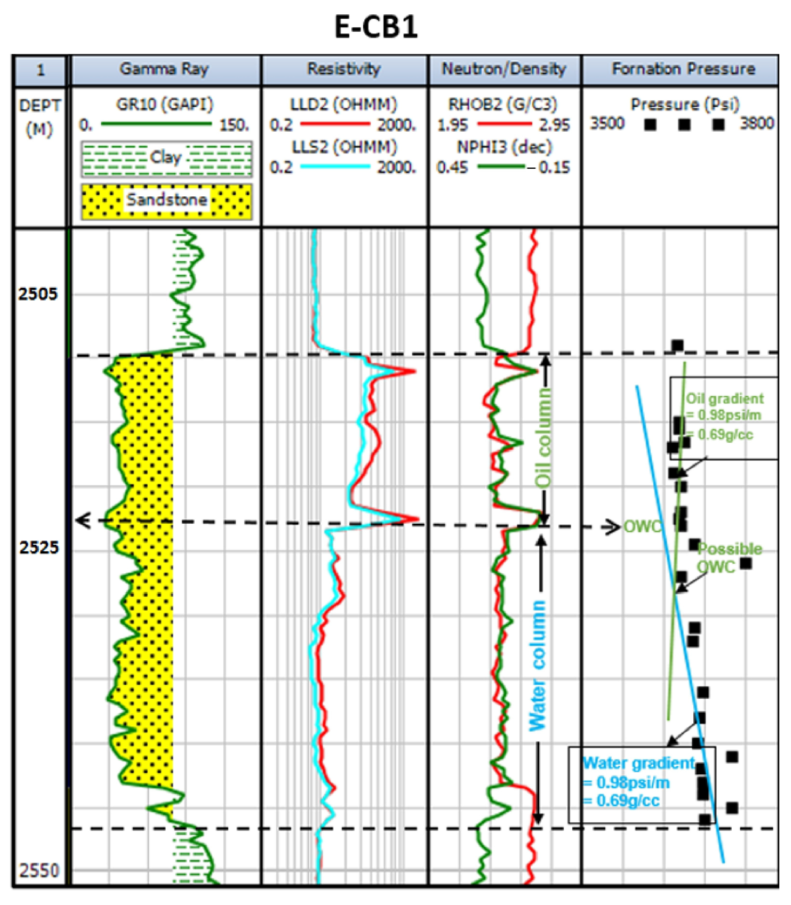
| Well | Water Gradient | Density (g/cc) | Oil Gradient | Density (g/cc) | Gas Gradient | Density (g/cc) |
|---|---|---|---|---|---|---|
| E-BK1 | – | – | – | – | 0.14 psi/ft | 0.32 |
| 0.45 psi/m | ||||||
| E-AJ1 | 0.44 psi/ft | 1.01 | 0.30 psi/ft | 0.69 | 0.1 psi/ft | 0.23 |
| 1.44 psi/m | 0.98 psi/m | 0.33 psi/m | ||||
| E-CB1 | 0.42 psi/ft | 0.97 | 0.26 psi/ft | 1.00 | – | – |
| 1.37 psi/m | 0.85 psi/m | |||||
| Average | 0.43 psi/ft | 0.99 | 0.28 psi/ft | 0.85 | 0.12 psi/ft | 0.28 |
| 1.41 psi/m | 0.92 psi/m | 0.39 psi/m |
| Well | Well Log GWC Depth (m) | RFT GWC Depth (m) | ||
| Resistivity | Neutron/Density | RFT | Observation | |
| EBK-1 | 2967.5 | 2967.5 | – | - |
| Well Log OWC Depth (m) | RFT OWC Depth (m) | |||
| Resistivity | Neutron/Density | RFT | Observation | |
| E-AJ1 | 2723 | 2723 | 2723 | Agreement |
| E-CB1 | 2523 | 2523 | 2528.5 | Disagreement |
| Well Log GOC Depth (m) | RFT GOC Depth (m) | |||
| Resistivity | Neutron/Density | RFT | Observation | |
| E-AJ1 | 2699 | 2699 | 2699 | Agreement |
Disclaimer/Publisher’s Note: The statements, opinions and data contained in all publications are solely those of the individual author(s) and contributor(s) and not of MDPI and/or the editor(s). MDPI and/or the editor(s) disclaim responsibility for any injury to people or property resulting from any ideas, methods, instructions or products referred to in the content. |
© 2025 by the authors. Licensee MDPI, Basel, Switzerland. This article is an open access article distributed under the terms and conditions of the Creative Commons Attribution (CC BY) license (https://creativecommons.org/licenses/by/4.0/).
Share and Cite
Shabangu, P.P.; Magoba, M.; Opuwari, M. Pore Pressure Prediction and Fluid Contact Determination: A Case Study of the Cretaceous Sediments in the Bredasdorp Basin, South Africa. Appl. Sci. 2025, 15, 7154. https://doi.org/10.3390/app15137154
Shabangu PP, Magoba M, Opuwari M. Pore Pressure Prediction and Fluid Contact Determination: A Case Study of the Cretaceous Sediments in the Bredasdorp Basin, South Africa. Applied Sciences. 2025; 15(13):7154. https://doi.org/10.3390/app15137154
Chicago/Turabian StyleShabangu, Phethile Promise, Moses Magoba, and Mimonitu Opuwari. 2025. "Pore Pressure Prediction and Fluid Contact Determination: A Case Study of the Cretaceous Sediments in the Bredasdorp Basin, South Africa" Applied Sciences 15, no. 13: 7154. https://doi.org/10.3390/app15137154
APA StyleShabangu, P. P., Magoba, M., & Opuwari, M. (2025). Pore Pressure Prediction and Fluid Contact Determination: A Case Study of the Cretaceous Sediments in the Bredasdorp Basin, South Africa. Applied Sciences, 15(13), 7154. https://doi.org/10.3390/app15137154