Integrating Probability and Possibility Theory: A Novel Approach to Valuing Real Options in Uncertain Environments


Abstract
Featured Application
Abstract
1. Introduction
2. Fuzzy Sets in Real Options Pricing
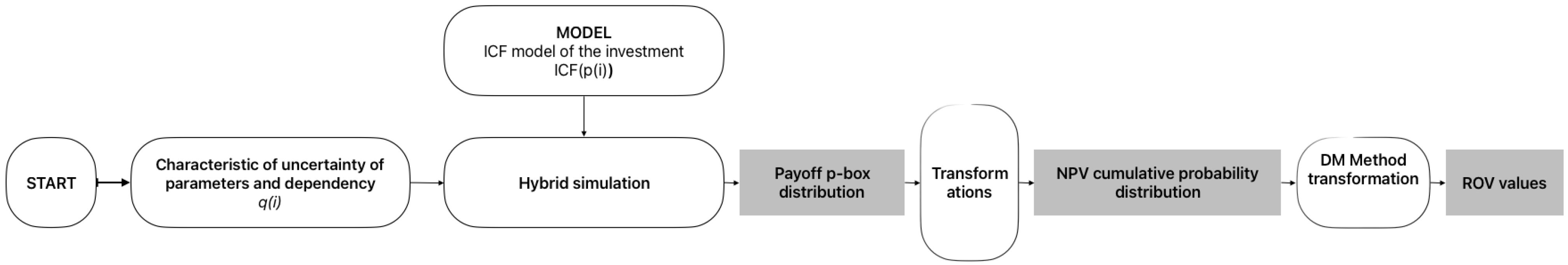
3. Materials and Methods
3.1. Modeling Uncertainty by Correlated Random–Fuzzy Geometric Brownian Motion (GBM)
3.2. Uncertainty Propagation
| Algorithm 1 Calculation of pay-off distribution in hybrid environment |
| Require: J, , T begin Set j = 0 while while calculate sup() and inf() of (,,0) (Equation (4)) subject to α-level constraints (Equations (8) and (9)) interdependence between (Equations (6) and (7)) for t = 0 to T−1 Generate vector of (MC Sampling with Cholesky decomposition) Forecast vector of (Equation (4)) Solve subject to financial constraints Solve subject to financial constraints Compute j = j + 1 end |
3.3. Transformation of p-Box into Subjective Pay-Off Distribution
3.4. Decision-Theoretic Scope and Limits
3.5. Datar–Mathews Method in Random–Fuzzy Environment
3.6. Comparison with Existing Approaches
4. Results
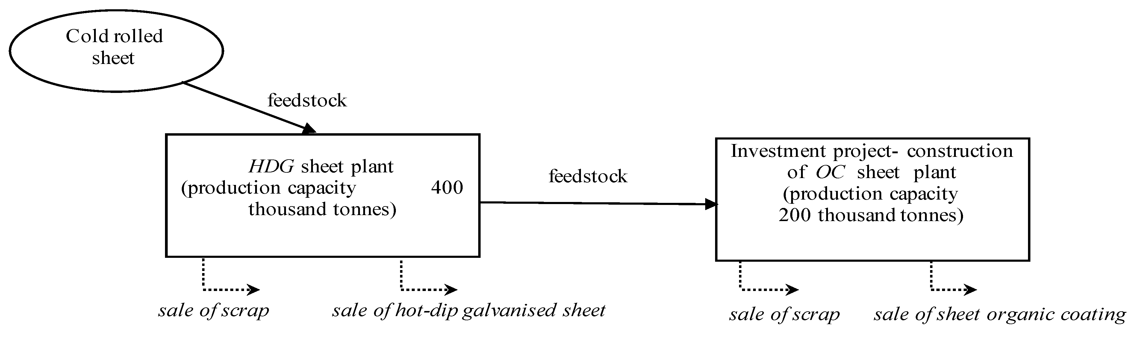
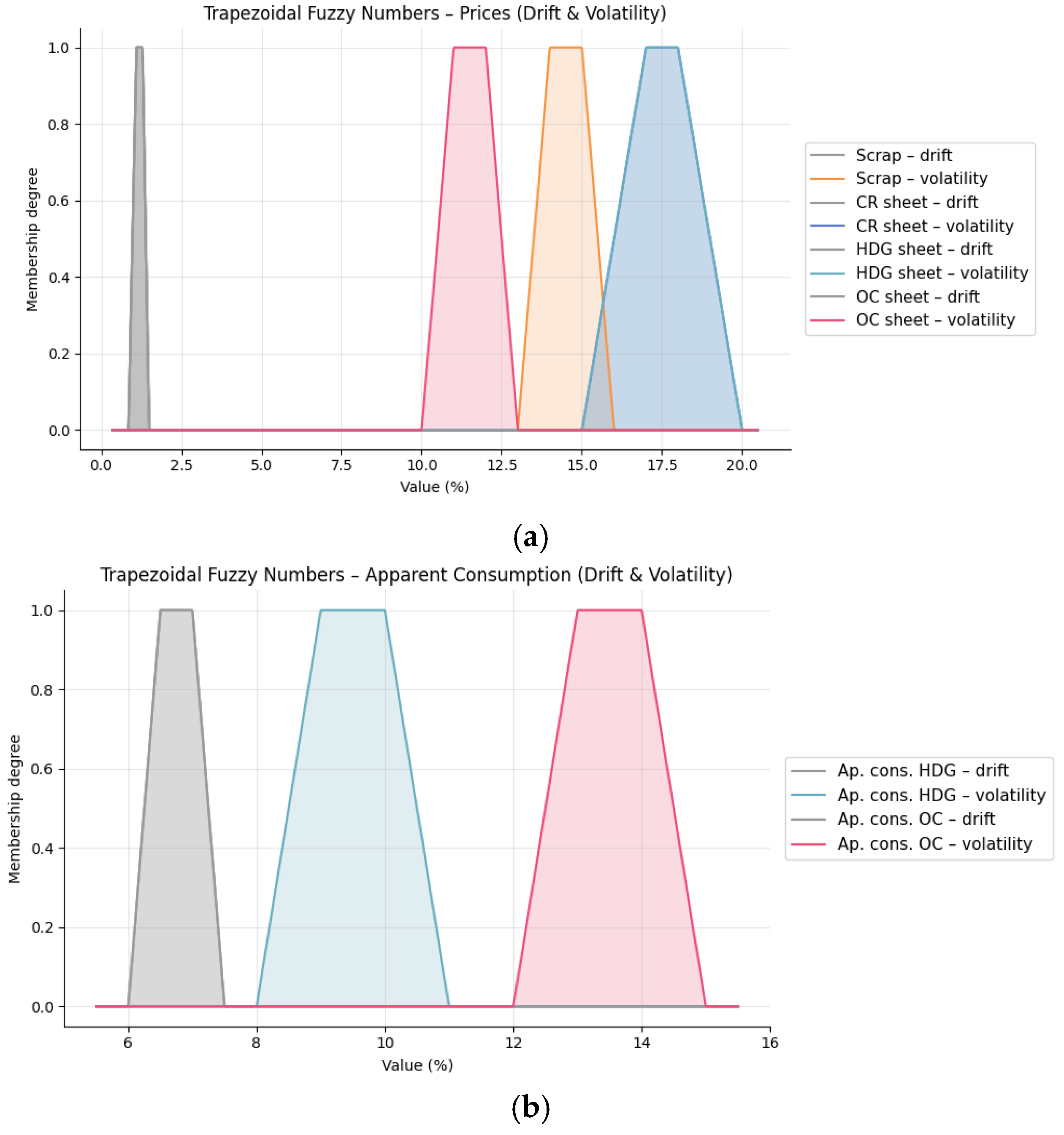
Model for Estimating the Value of Project in Hybrid Environment
- Prices
- Scrap: (13.0%, 14.0%, 15.0%, 16.0%);
- CR sheet and HDG sheet: (15.0%, 17.0%, 18.0%, 20.0%);
- OC sheet: (10.0%, 11.0%, 12.0%, 13.0%).
- Apparent consumption
- HDG sheet: (8.0%, 9.0%, 10.0%, 11.0%);
- OC sheet: (12.0%, 13.0%, 14.0%, 15.0%).
5. Discussion
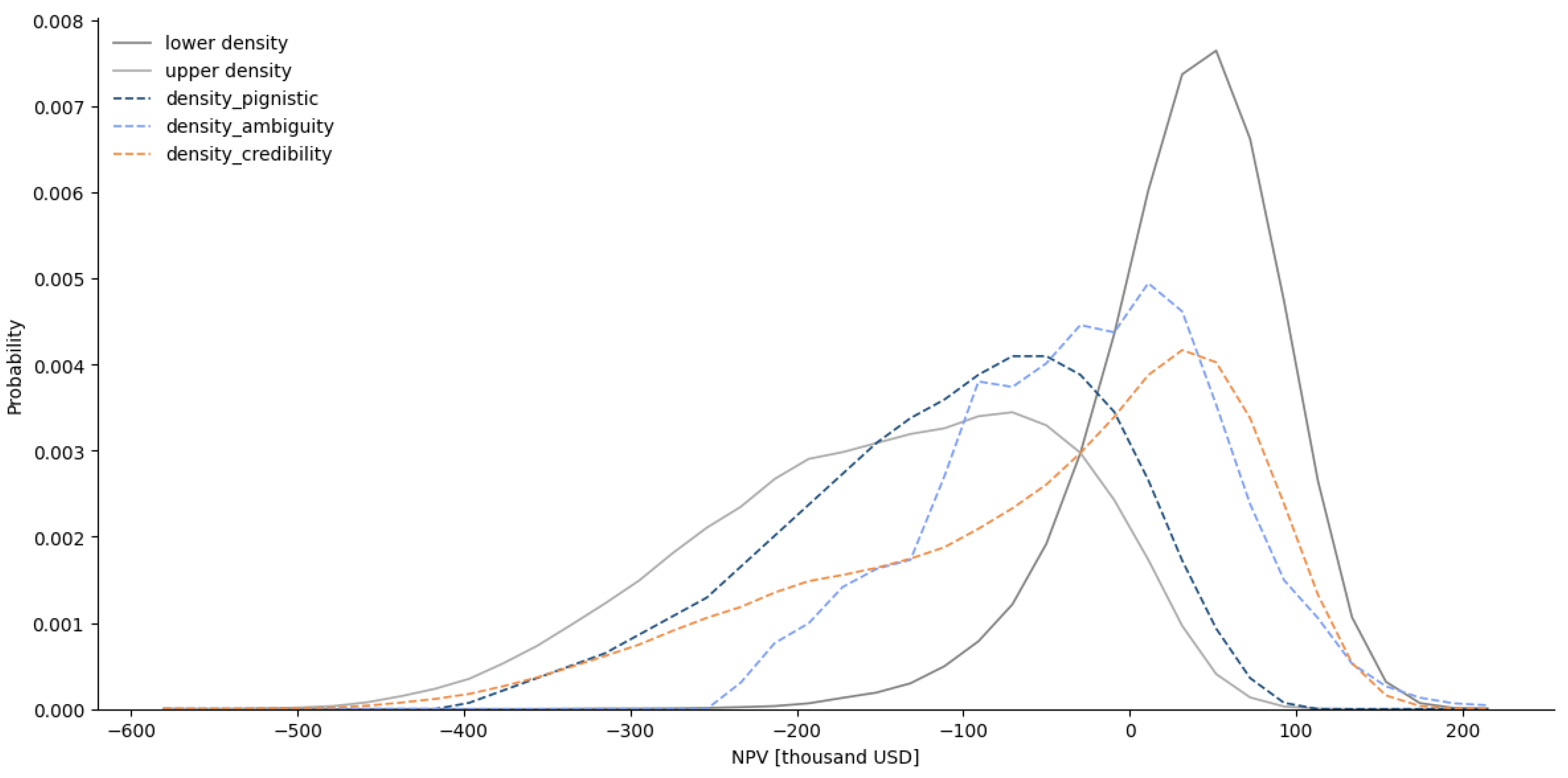
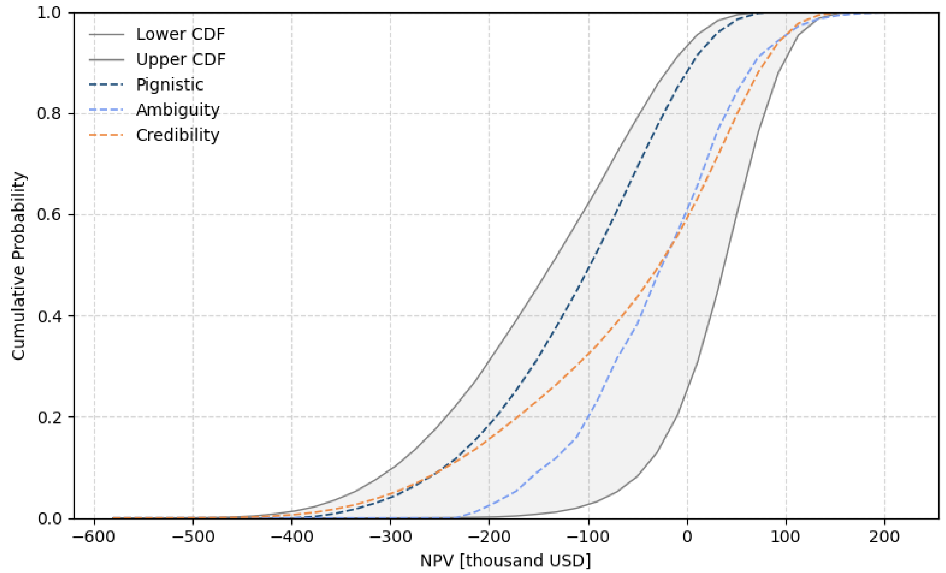
5.1. Decomposition of Epistemic and Aleatory Uncertainty
5.2. Hybrid Real Option Valuation Results
5.3. Benchmarking Against the Fuzzy Pay-Off Method
6. Conclusions
6.1. Managerial Insigts
6.2. Practical Advantages and Competitiveness of the Hybrid Random–Fuzzy DMM
Author Contributions
Funding
Institutional Review Board Statement
Informed Consent Statement
Data Availability Statement
Acknowledgments
Conflicts of Interest
References
- Mathews, S.; Datar, V.; Johnson, B. A Practical Method for Valuing Real Options: The Boeing Approach. J. Appl. Corp. Financ. 2007, 19, 95–104. [Google Scholar] [CrossRef]
- Datar, V.T.; Mathews, S.H. European Real Options: An Intuitive Algorithm for the Black-Scholes Formula. 2005. Available online: https://papers.ssrn.com/sol3/papers.cfm?abstract_id=560982 (accessed on 1 April 2025).
- Collan, M. Thoughts about Selected Models for the Valuation of Real Options. Acta Univ. Palacki. Olomuc. Fac. Rerum Nat. Math. 2011, 50, 5–12. [Google Scholar]
- de Magalhães Ozorio, L.; Bastian-Pinto, C.d.L.; Baidya, T.K.N.; Brandão, L.E.T. Investment Decision in Integrated Steel Plants under Uncertainty. Int. Rev. Financ. Anal. 2013, 27, 55–64. [Google Scholar] [CrossRef]
- Rębiasz, B.; Gaweł, B.; Skalna, I. Valuing Managerial Flexibility: An Application of Real-Option Theory to Steel Industry Investments. Oper. Res. Decis. 2017, 27, 91–111. [Google Scholar] [CrossRef]
- Wu, H.-C. Using Fuzzy Sets Theory and Black–Scholes Formula to Generate Pricing Boundaries of European Options. Appl. Math. Comput. 2007, 185, 136–146. [Google Scholar] [CrossRef]
- Zmeškal, Z. Generalised Soft Binomial American Real Option Pricing Model (Fuzzy–Stochastic Approach). Eur. J. Oper. Res. 2010, 207, 1096–1103. [Google Scholar] [CrossRef]
- Carlsson, C.; Fullér, R. A Fuzzy Approach to Real Option Valuation. Fuzzy Sets Syst. 2003, 139, 297–312. [Google Scholar] [CrossRef]
- de Andrés-Sánchez, J. A Systematic Review of the Interactions of Fuzzy Set Theory and Option Pricing. Expert Syst. Appl. 2023, 223, 119868. [Google Scholar] [CrossRef]
- Guerra, M.L.; Magni, C.A.; Stefanini, L. Value Creation and Investment Projects: An Application of Fuzzy Sensitivity Analysis To Project Financing Transactions. Int. J. Inf. Technol. Decis. Mak. 2022, 26, 1683–1714. [Google Scholar] [CrossRef]
- Wu, H.-C. Pricing European Options Based on the Fuzzy Pattern of Black–Scholes Formula. Comput. Oper. Res. 2004, 31, 1069–1081. [Google Scholar] [CrossRef]
- Lee, C.-F.; Tzeng, G.-H.; Wang, S.-Y. A New Application of Fuzzy Set Theory to the Black–Scholes Option Pricing Model. Expert Syst. Appl. 2005, 29, 330–342. [Google Scholar] [CrossRef]
- Gaweł, B.; Paliński, A. Long-Term Natural Gas Consumption Forecasting Based on Analog Method and Fuzzy Decision Tree. Energies 2021, 14, 4905. [Google Scholar] [CrossRef]
- Paliński, A. Opcje rzeczywiste w podejmowaniu decyzji inwestycyjnych na przykładzie budowy podziemnego magazynu gazu. Naft.-Gaz 2016, 72, 33–39. [Google Scholar] [CrossRef]
- Black, F.; Scholes, M. The Pricing of Options and Corporate Liabilities. J. Polit. Econ. 1973, 81, 637–654. [Google Scholar] [CrossRef]
- Cox, J.C.; Ross, S.A.; Rubinstein, M. Option Pricing: A Simplified Approach. J. Financ. Econ. 1979, 7, 229–263. [Google Scholar] [CrossRef]
- Brandão, L.; Dyer, J.; Hahn, W. Using Binomial Decision Trees to Solve Real-Option Valuation Problems. Decis. Anal. 2005, 2, 69–88. [Google Scholar] [CrossRef]
- Collan, M.; Fuller, R.; Mezei, J. A Fuzzy Pay-Off Method for Real Option Valuation. In Proceedings of the 2009 International Conference on Business Intelligence and Financial Engineering, Beijing, China, 24–26 July 2009; pp. 165–169. [Google Scholar]
- Huang, M.-G. Real Options Approach-Based Demand Forecasting Method for a Range of Products with Highly Volatile and Correlated Demand. Eur. J. Oper. Res. 2009, 198, 867–877. [Google Scholar] [CrossRef]
- Xu, W.; Wu, C.; Xu, W.; Li, H. A Jump-Diffusion Model for Option Pricing under Fuzzy Environments. Insur. Math. Econ. 2009, 44, 337–344. [Google Scholar] [CrossRef]
- Knight, F. Risk, Uncertainty and Profit; Vernon Press Titles in Economics: Wilmington, DE, USA, 2013. [Google Scholar]
- Howard, R.A. Decision Analysis: Applied Decision Theory; Stanford Research Institute: Menlo Park, CA, USA, 1966. [Google Scholar]
- Dixit, A.K.; Pindyck, R.S. Investment Under Uncertainty; Princeton University Press: Princeton, NJ, USA, 1994; ISBN 978-0-691-03410-2. [Google Scholar]
- Carlsson, C.; Fullér, R.; Heikkilä, M.; Majlender, P. A Fuzzy Approach to R&D Project Portfolio Selection. Int. J. Approx. Reason. 2007, 44, 93–105. [Google Scholar] [CrossRef]
- Augusto Alcaraz Garcia, F. Fuzzy Real Option Valuation in a Power Station Reengineering Project. In Proceedings of the Proceedings World Automation Congress, 2004, Seville, Spain, 28 June–1 July 2004; Volume 17, pp. 281–288. [Google Scholar]
- Allenotor, D.; Thulasiram, R.K. A Grid Resources Valuation Model Using Fuzzy Real Option. In Parallel and Distributed Processing and Applications; Stojmenovic, I., Thulasiram, R.K., Yang, L.T., Jia, W., Guo, M., de Mello, R.F., Eds.; Springer: Berlin/Heidelberg, Germany, 2007; pp. 622–632. [Google Scholar]
- Tao, C.; Jinlong, Z.; Shan, L.; Benhai, Y. Fuzzy Real Option Analysis for IT Investment in Nuclear Power Station. In Computational Science—ICCS 2007; Shi, Y., van Albada, G.D., Dongarra, J., Sloot, P.M.A., Eds.; Springer: Berlin/Heidelberg, Germany, 2007; pp. 953–959. [Google Scholar]
- Zeng, M.; Wang, H.; Zhang, T.; Li, B.; Huang, S. Research and Application of Power Network Investment Decision-Making Model Based on Fuzzy Real Options. In Proceedings of the 2007 International Conference on Service Systems and Service Management, Chengdu, China, 9–11 June 2007; pp. 1–5. [Google Scholar]
- Uçal, İ.; Kahraman, C. Fuzzy Real Options Valuation for Oil Investments. Ukio Technol. Ekon. Vystym. 2009, 15, 646–669. [Google Scholar] [CrossRef]
- Ho, S.-H.; Liao, S.-H. A Fuzzy Real Option Approach for Investment Project Valuation. Expert Syst. Appl. 2011, 38, 15296–15302. [Google Scholar] [CrossRef]
- Zmeškal, Z.; Dluhošová, D.; Gurný, P.; Kresta, A. Generalised Soft Multi-Mode Real Options Model (Fuzzy-Stochastic Approach). Expert Syst. Appl. 2022, 192, 116388. [Google Scholar] [CrossRef]
- Maier, S.; Pflug, G.C.; Polak, J.W. Valuing Portfolios of Interdependent Real Options under Exogenous and Endogenous Uncertainties. Eur. J. Oper. Res. 2020, 285, 133–147. [Google Scholar] [CrossRef]
- de Andrés-Sánchez, J. A Systematic Overview of Fuzzy-Random Option Pricing in Discrete Time and Fuzzy-Random Binomial Extension Sensitive Interest Rate Pricing. Axioms 2025, 14, 52. [Google Scholar] [CrossRef]
- Kozlova, M.; Collan, M.; Luukka, P. Comparison of the Datar-Mathews Method and the Fuzzy Pay-Off Method through Numerical Results. Adv. Decis. Sci. 2016, 2016, 7836784. [Google Scholar] [CrossRef]
- Borges, R.E.P.; Dias, M.A.G.; Dória Neto, A.D.; Meier, A. Fuzzy Pay-off Method for Real Options: The Center of Gravity Approach with Application in Oilfield Abandonment. Fuzzy Sets Syst. 2018, 353, 111–123. [Google Scholar] [CrossRef]
- Stoklasa, J.; Luukka, P.; Collan, M. Possibilistic Fuzzy Pay-off Method for Real Option Valuation with Application to Research and Development Investment Analysis. Fuzzy Sets Syst. 2021, 409, 153–169. [Google Scholar] [CrossRef]
- Stoklasa, J.; Collan, M.; Luukka, P. Practical Possibilistic Fuzzy Pay-off Method for Real Option Valuation. Fuzzy Sets Syst. 2024, 492, 109072. [Google Scholar] [CrossRef]
- Tannenbaum, D.; Fox, C.R.; Ülkümen, G. Judgment Extremity and Accuracy Under Epistemic vs. Aleatory Uncertainty. Manag. Sci. 2017, 63, 497–518. [Google Scholar] [CrossRef]
- Walters, D.J.; Ülkümen, G.; Tannenbaum, D.; Erner, C.; Fox, C.R. Investor Behavior Under Epistemic vs. Aleatory Uncertainty. Manag. Sci. 2023, 69, 2761–2777. [Google Scholar] [CrossRef]
- Wattanarat, V.; Phimphavong, P.; Matsumaru, M. Demand and Price Forecasting Models for Strategic and Planning Decisions in a Supply Chain. Proc. Sch. Inf. Telecommun. Eng. Tokai Univ. 2010, 3, 37–42. [Google Scholar]
- Bastian-Pinto, C.; Brandão, L.; Hahn, W.J. Flexibility as a Source of Value in the Production of Alternative Fuels: The Ethanol Case. Energy Econ. 2009, 31, 411–422. [Google Scholar] [CrossRef]
- Marathe, R.R.; Ryan, S.M. On The Validity of The Geometric Brownian Motion Assumption. Eng. Econ. 2005, 50, 159–192. [Google Scholar] [CrossRef]
- Dubois, D.; Prade, H. Practical Methods for Constructing Possibility Distributions. Int. J. Intell. Syst. 2016, 31, 215–239. [Google Scholar] [CrossRef]
- Rebiasz, B. New Methods of Probabilistic and Possibilistic Interactive Data Processing. J. Intell. Fuzzy Syst. 2016, 30, 2639–2656. [Google Scholar] [CrossRef]
- Yang, I.-T. Simulation-Based Estimation for Correlated Cost Elements. Int. J. Proj. Manag. 2005, 23, 275–282. [Google Scholar] [CrossRef]
- Hladík, M.; Černý, M. Interval Regression by Tolerance Analysis Approach. Fuzzy Sets Syst. 2012, 193, 85–107. [Google Scholar] [CrossRef]
- Clavreul, J.; Guyonnet, D.; Tonini, D.; Christensen, T.H. Stochastic and Epistemic Uncertainty Propagation in LCA. Int. J. Life Cycle Assess. 2013, 18, 1393–1403. [Google Scholar] [CrossRef]
- Guyonnet, D.; Coftier, A.; Bataillard, P.; Destercke, S. Risk-Based Imprecise Post-Remediation Soil Quality Objectives. Sci. Total Environ. 2024, 923, 171445. [Google Scholar] [CrossRef]
- Islam, M.S.; Nepal, M.P.; Skitmore, M.; Attarzadeh, M. Current Research Trends and Application Areas of Fuzzy and Hybrid Methods to the Risk Assessment of Construction Projects. Adv. Eng. Inform. 2017, 33, 112–131. [Google Scholar] [CrossRef]
- Baudrit, C.; Dubois, D.; Guyonnet, D. Joint Propagation and Exploitation of Probabilistic and Possibilistic Information in Risk Assessment. IEEE Trans. Fuzzy Syst. 2006, 14, 593–608. [Google Scholar] [CrossRef]
- Rȩbiasz, B.; Gaweł, B.; Skalna, I. Hybrid Framework for Investment Project Portfolio Selection. In Advances in Business ICT: New Ideas from Ongoing Research; Pełech-Pilichowski, T., Mach-Król, M., Olszak, C.M., Eds.; Studies in Computational Intelligence; Springer International Publishing: Cham, Switzerland, 2017; pp. 87–104. ISBN 978-3-319-47208-9. [Google Scholar]
- Gaweł, B.; Rębiasz, B.; Skalna, I. Teoria Prawdopodobieństwa i Teoria Możliwości w Podejmowaniu Decyzji Inwestycyjnych. Stud. Ekon. 2015, 248, 62–79. [Google Scholar]
- Wakker, P.P. Prospect Theory: For Risk and Ambiguity; Cambridge University Press: Cambridge, UK, 2010; ISBN 978-1-139-48910-2. [Google Scholar]
- Schröder, D. Real Options, Ambiguity, and Dynamic Consistency—A Technical Note. Int. J. Prod. Econ. 2020, 229, 107772. [Google Scholar] [CrossRef]
- Dubois, D.; Prade, H. Possibility Theory and Its Applications: Where Do We Stand? In Springer Handbook of Computational Intelligence; Kacprzyk, J., Pedrycz, W., Eds.; Springer Handbooks; Springer: Berlin/Heidelberg, Germany, 2015; pp. 31–60. ISBN 978-3-662-43505-2. [Google Scholar]
- Dubois, D.; Prade, H.; Smets, P. A Definition of Subjective Possibility. Int. J. Approx. Reason. 2008, 48, 352–364. [Google Scholar] [CrossRef]
- Smets, P. Decision Making in the TBM: The Necessity of the Pignistic Transformation. Int. J. Approx. Reason. 2005, 38, 133–147. [Google Scholar] [CrossRef]
- Dubois, D.; Guyonnet, D. Risk-Informed Decision-Making in the Presence of Epistemic Uncertainty. Int. J. Gen. Syst. 2011, 40, 145–167. [Google Scholar] [CrossRef]
- Liu, B. Uncertainty Theory; Springer Uncertainty Research; Springer: Berlin/Heidelberg, Germany, 2015; ISBN 978-3-662-44353-8. [Google Scholar]
- Yang, X.; Li, C.; Li, X.; Lu, Z. A Parallel Monte Carlo Algorithm for the Life Cycle Asset Allocation Problem. Appl. Sci. 2024, 14, 10372. [Google Scholar] [CrossRef]
- Ferson, S.; Kreinovick, V.; Ginzburg, L.; Sentz, F. Constructing Probability Boxes and Dempster-Shafer Structures; Sandia National Laboratories: Albuquerque, NM, USA, 2003. [Google Scholar]
- Dubois, D.; Prade, H. A Fresh Look at Z-Numbers—Relationships with Belief Functions and p-Boxes. Fuzzy Inf. Eng. 2018, 10, 5–18. [Google Scholar] [CrossRef]
- Pianosi, F.; Wagener, T. A Simple and Efficient Method for Global Sensitivity Analysis Based on Cumulative Distribution Functions. Environ. Model. Softw. 2015, 67, 1–11. [Google Scholar] [CrossRef]
- Ferson, S.; Oberkampf, W.L. Validation of Imprecise Probability Models. Int. J. Reliab. Saf. 2009, 3, 3–22. [Google Scholar] [CrossRef]
- He, Q. Model Validation Based on Probability Boxes under Mixed Uncertainties. Adv. Mech. Eng. 2019, 11, 1687814019847411. [Google Scholar] [CrossRef]
- Skalna, I.; Rebiasz, B.; Gawel, B.; Basiura, B.; Duda, J.; Opila, J.; Pelech-Pilichowski, T. Advances in Fuzzy Decision Making; Studies in Fuzziness and Soft Computing; Springer: Cham, Switzerland, 2015; Volume 333. [Google Scholar]
- Bowman, E.H.; Hurry, D. Strategy through the Option Lens: An Integrated View of Resource Investments and the Incremental-Choice Process. Acad. Manag. Rev. 1993, 18, 760–782. [Google Scholar] [CrossRef]
- Burger-Helmchen, T. Option Chain and Change Management: A Structural Equation Application. Eur. Manag. J. 2009, 27, 176–186. [Google Scholar] [CrossRef]
- Exploring the Usefulness of Real Options Theory for Foreign Affiliate Divestments: Real Abandonment Options’ Applications. Available online: https://www.mdpi.com/1911-8074/17/10/438 (accessed on 11 June 2025).

| Indices |
| t—investment period: {1, …, T}; scen—scenario: base—baseline, inv—investment; prod—product: OC—OC sheet, HDG—HDG sheet, CR—CR sheet, scrap—scrap; |
| Input parameters |
| TA—tax, —capacity of prod plan; —market share of prod product; DTR—receivable turnover ratio; CTR—cash turnover ratio; ITO—inventory turnover ratio; DTP—payable turnover ratio; PUCprod—per-unit consumption of sheet required to produce prod sheet; —fixed cost of prod plan; —other annual variable production costs per ton for prod sheet; Auxiliary variables —profit after tax in scen scenario in t; —annual depreciation of prod plan in t; —the change in net working capital in scen scenario in t; —residual value in scen scenario in T; —revenue in scen scenario in t; —total cost in scen scenario in t; —sales volume of prod product in scen scenario in t; —net working capital in year t in scenario scen; —cost of CR sheet per ton of prod sheet in year t; —sales forecast for prod product; |
| Uncertain variables |
| —price of prod per ton in year t; —apparent consumption forecast for prod product in t. |
| Scrap | CR Sheet | HDG Sheet | OC Sheet | |
|---|---|---|---|---|
| Scrap | 1.000 | 0.955 | 0.892 | 0.853 |
| CR sheet | 0.955 | 1.000 | 0.961 | 0.921 |
| HDG sheet | 0.892 | 0.961 | 1.000 | 0.911 |
| OC sheet | 0.853 | 0.921 | 0.911 | 1.000 |
| Independent Variable | Dependent Variable | ||||
|---|---|---|---|---|---|
| Scrap | CR Sheet | HDG Sheet | OC Sheet | ||
| Scrap | a1 | [−0.060; 1.943] | [0.369; 1.378] | [0.589; 1.554] | |
| a2 | [−0.018; 0.001] | [−0.006; −0.002] | [0.003; 0.0098] | ||
| CR sheet | a1 | [−0.897; 2.914] | [−1.611; 3.287] | [−1.689; 3.951] | |
| a2 | [−0.013; 0.041] | [−0.015; 0.039] | [−0.031; 0.069] | ||
| HDG sheet | a1 | [0.721; 1.489] | [0.399; 1.598] | [0.531; 1.811] | |
| a2 | [0.003; 0.006] | [−0.011; −0.003] | [0.004; 0.016] | ||
| OC sheet | a1 | [0.063; 1.689 | [−2.160; 3.866] | [−0.599; 2.112] | |
| a2 | [−0.012; 0.003] | [−0.062; 0.040] | [−0.022; 0.007] | ||
| Independent Variable | Dependent Variable | ||
|---|---|---|---|
| HDG Sheet | OC Sheet | ||
| HDG sheet | a1 | [−0.239; 0.800] | |
| a2 | [−0.050; 0.167] | ||
| OC sheet | a1 | [−1.589; 3.461] | |
| a2 | [−0.040; 0.088] | ||
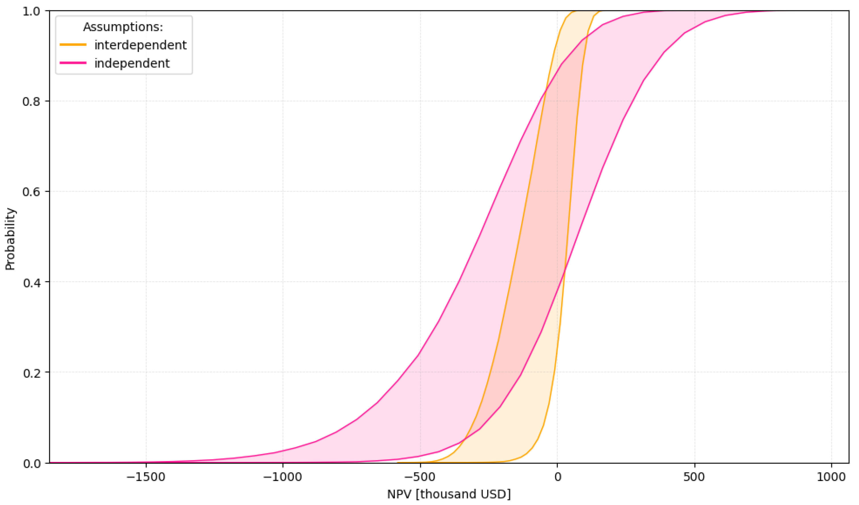
| Assumption | Δmax | npv* | Area A | |
|---|---|---|---|---|
| Interdependent (a) | 0.73 | −29,642 | 1.79 × 10⁵ | 0.22 |
| Independent (b) | 0.52 | −133,037 | 3.87 × 10⁵ | 0.13 |
| Assumption | Smean | IQR |
|---|---|---|
| Interdependent (a) | 2.51 × 10⁻⁶ | 180 |
| Independent (b) | 1.00 × 10⁻⁶ | 434 |
| E(npv) | −3.42 USD | 1.05 USD | −2.48 USD | −492 USD | −1.18 USD |
| Std dev | 4.13 USD | 3.16 USD | 3.45 USD | 2603 USD | 3.06 USD |
| Success ratio | 8% | 80% | 15% | 54% | 55% |
| ROV | 2.41 USD | 50.91 USD | 4.60 USD | 23.72 USD | 26.66 USD |
Disclaimer/Publisher’s Note: The statements, opinions and data contained in all publications are solely those of the individual author(s) and contributor(s) and not of MDPI and/or the editor(s). MDPI and/or the editor(s) disclaim responsibility for any injury to people or property resulting from any ideas, methods, instructions or products referred to in the content. |
© 2025 by the authors. Licensee MDPI, Basel, Switzerland. This article is an open access article distributed under the terms and conditions of the Creative Commons Attribution (CC BY) license (https://creativecommons.org/licenses/by/4.0/).
Share and Cite
Gaweł, B.; Rębiasz, B.; Paliński, A. Integrating Probability and Possibility Theory: A Novel Approach to Valuing Real Options in Uncertain Environments. Appl. Sci. 2025, 15, 7143. https://doi.org/10.3390/app15137143
Gaweł B, Rębiasz B, Paliński A. Integrating Probability and Possibility Theory: A Novel Approach to Valuing Real Options in Uncertain Environments. Applied Sciences. 2025; 15(13):7143. https://doi.org/10.3390/app15137143
Chicago/Turabian StyleGaweł, Bartłomiej, Bogdan Rębiasz, and Andrzej Paliński. 2025. "Integrating Probability and Possibility Theory: A Novel Approach to Valuing Real Options in Uncertain Environments" Applied Sciences 15, no. 13: 7143. https://doi.org/10.3390/app15137143
APA StyleGaweł, B., Rębiasz, B., & Paliński, A. (2025). Integrating Probability and Possibility Theory: A Novel Approach to Valuing Real Options in Uncertain Environments. Applied Sciences, 15(13), 7143. https://doi.org/10.3390/app15137143