EKNet: Graph Structure Feature Extraction and Registration for Collaborative 3D Reconstruction in Architectural Scenes

Abstract

Collaborative geometric reconstruction of building structures can significantly reduce communication consumption for data sharing, protect privacy, and provide support for large-scale robot application management. In recent years, geometric reconstruction of building structures has been partially studied, but there is a lack of alignment fusion studies for multi-UAV (Unmanned Aerial Vehicle)-reconstructed geometric structure models. The vertices and edges of geometric structure models are sparse, and existing methods face challenges such as low feature extraction efficiency and substantial data requirements when processing sparse graph structures after geometrization. To address these challenges, this paper proposes an efficient deep graph matching registration framework that effectively integrates interpretable feature extraction with network training. Specifically, we first extract multidimensional local properties of nodes by combining geometric features with complex network features. Next, we construct a lightweight graph neural network, named EKNet, to enhance feature representation capabilities, enabling improved performance in low-overlap registration scenarios. Finally, through feature matching and discrimination modules, we effectively eliminate incorrect pairings and enhance accuracy. Experiments demonstrate that the proposed method achieves a 27.28% improvement in registration speed compared to traditional GCN (Graph Convolutional Neural Networks) and an 80.66% increase in registration accuracy over the suboptimal method. The method exhibits strong robustness in registration for scenes with high noise and low overlap rates. Additionally, we construct a standardized geometric point cloud registration dataset.

1. Introduction

Three-dimensional (3D) reconstruction as integrated in UAV remote sensing is one of the important research directions in the field of computer vision [1,2]. It plays a critical role in key domains such as fire and emergency rescue operations [3], the construction of smart cities [4], and counter-terrorism initiatives, where there is an urgent need for rapid reconstruction and lightweight transmission of building scenes. Although the current deep learning models can meet the basic needs of UAV remote sensing, their consumption of computational resources and storage capacity tends to be high. There is also an urgent need for fast data acquisition, efficient transmission, and accurate processing. Geometric reconstruction of point cloud data can achieve more efficient transmission, processing, and storage while meeting application requirements. At the same time, the multi-UAV cooperative operation mode can effectively meet the demand for rapid automated reconstruction of large-scale building scenes such as office buildings, train stations, and shopping malls. Although multi-UAV cooperative construction can significantly improve the reconstruction efficiency, the point cloud data collected by each device has the problem of involving an inconsistent coordinate system. Additionally, the distribution of vertices after geometric reconstruction tends to be sparse and noisy [5,6], complicating the direct alignment of reconstruction results from different device nodes using vertex coordinates. To fully leverage the prominent edge relationships in geometric reconstruction results, this paper introduces, for the first time, an efficient and accurate graph-based structural alignment method aimed at achieving precise alignment of reconstruction outcomes from multiple UAVs.

In the current research, the methodologies for point cloud registration and map registration exhibit significant similarities, particularly with regards to deep learning-based approaches and point correspondence techniques, which are widely employed and hold substantial reference value [7,8,9,10,11,12]. The primary objective of point cloud registration is to align disparate point clouds into a unified coordinate system [13]. Similarly, graph structure registration aims to align multiple frames of graph structure data within the same coordinate system, ensuring consistent spatial positions and orientations. This process typically entails the computation of a rotation matrix and a translation matrix to achieve optimal alignment among multiple partially overlapping images. In recent years, advancements in point cloud neural network feature extraction technology and differentiable optimization techniques have progressed rapidly. Consequently, the compressed processing method for point cloud registration has emerged as a focal point of research, driven by the constraints of communication conditions and the increasing demands for processing speed and data volume [14].

Most point-to-point relationship strategies rely on identifying key points to establish correspondences [15,16]. The trained neural network identifies the point pair relationships between two input point clouds and then employs robust estimation methods, such as the RANSAC algorithm [17], to determine the optimal alignment between them. However, a significant challenge persists in compressing data transmission while enhancing the effectiveness of point cloud features, particularly when the overlapping area is minimal. To address this issue, some studies have utilized deep learning techniques to obtain more efficient representations of point cloud features and have developed point matching algorithms to establish correspondences between points [18]. Subsequently, the rotation matrix ${\displaystyle R}$ and translation matrix ${\displaystyle T}$ are computed using the Singular Value Decomposition (SVD) algorithm, which has markedly improved the accuracy, robustness, and speed of point cloud registration [19]. These methods also incorporate strategies inspired by traditional point cloud registration techniques. However, these approaches typically assume a perfect one-to-one correspondence between the source and target point clouds during the training phase, making them less robust when faced with noise and non-overlapping areas. In practical engineering applications, the registration task is further complicated by factors such as acquisition time, angle, sensor noise, and variations between sensors [20]. Moreover, while significant progress has been made in enhancing the accuracy of point cloud registration, relatively little research has concentrated on optimizing registration speed. Additionally, the consumption of execution time and the storage requirements for point cloud data volumes have also received limited attention.

Among the methods for feature extraction and processing in graph-structured data, mainstream technologies primarily utilize neural network models to learn the feature representations of nodes and edges. Specifically, the Graph Convolutional Network (GCN) [21] updates the feature representation of nodes by aggregating information from neighboring nodes. This process involves convolution operations that utilize the adjacency matrix and the node feature matrix of the graph. Additionally, graph kernel-based methods [22] achieve feature extraction by defining kernel functions between graphs to calculate their similarity. However, these methods encounter efficiency challenges when processing large-scale graph data. This inefficiency is primarily due to the high computational cost associated with calculating kernel functions between graphs. Furthermore, graph kernel methods lack flexibility in addressing dynamic changes in graph structures, as they predominantly focus on the static structural characteristics of graphs.

DeepWalk [23] and Node2Vec [24], both of which rely on random walks, may encounter limitations in memory and computational resources when processing large-scale graph data. This is due to the substantial resource requirements for generating node sequences with these methods and for subsequent model training. Furthermore, matrix factorization-based methods [25] may also experience challenges related to computational efficiency and memory usage when handling large-scale graph data. These approaches often struggle to effectively capture the local structural characteristics of graphs.

This paper proposes a drawing structure registration method for building structures, aimed at achieving efficient and high-precision feature extraction and registration with limited point cloud data volume. The method integrates manual feature extraction with graph neural network-based feature extraction to enhance the robustness and accuracy of the registration process. To address the challenge of excessive point cloud data volume, a topological processing method for point cloud data is introduced. This approach offers the advantages of rapid processing and reduced data transmission, making it suitable for scenarios with constrained communication conditions. By pre-processing the topologized point cloud data on local devices, the proposed method can achieve high-precision registration while significantly minimizing data transmission requirements. This approach not only improves computational efficiency but also ensures that the registration process remains effective even in resource-limited environments.

To address the challenges mentioned above, this paper proposes a method for registering drawing structures in building designs. The primary contributions of this work are summarized as follows:

• A point cloud registration framework based on feature metric geometry is introduced. This framework ensures high accuracy while enhancing improving computational efficiency. Compared with the Graph Convolutional Network (GCN) method, the proposed framework achieves a 27.28% improvement computational efficiency.
• A graph-structured, multidimensional feature construction module has been designed. By integrating geometric features with complex network indicators, this module significantly enhances the robustness of the registration results.
• A lightweight graph neural network, EKNet, has been developed. With an overlap rate of 20%, EKNet achieves a registration accuracy that is 80.66% higher than that of the sub-optimal method.
• Open-source GPCR, a geometric point cloud registration dataset for building structures, is now available. This dataset is distinguished by its extensive scale and diversity, providing substantial support for advancing research and development in the field.

2. Related Work

2.1. Registration Methods

In registration research, three main approaches currently prevail: methods based on original point information, methods based on feature points, and methods based on deep learning.

2.1.1. Original-Point-Information-Based Methods

ICP (Iterated Closest Point)-like methods optimize the distance error between points and achieve point cloud registration through iterative processes. These methods directly utilize the original point cloud information, specifically the three-dimensional coordinates, for registration. The Iterative Closest Point algorithm (ICP), proposed by Besl et al. [26], reformulates the point cloud registration problem as a least-squares optimization task. It iteratively computes the optimal registration transformation matrix T until the error is minimized. ICP has numerous variants, such as employing KD-tree [27] to partition the point cloud subspace for accelerated nearest-point queries and integrating the Random Sample Consensus (RANSAC) algorithm [17] to eliminate mismatched point pairs, thereby enhancing registration accuracy. Additionally, Chetverikov et al. introduced Trimmed ICP [28], which determines the number of points retained based on the overlap ratio of the point clouds. By performing transformation calculations using only the retained point pairs, Trimmed ICP improves the registration accuracy of partially overlapping point clouds. Beyond ICP-like methods, Campbell et al. [29] proposed a point cloud registration method based on a global probabilistic model. This approach reformulates the point cloud registration problem as the maximization of a probabilistic model. Specifically, the Von Mises Distribution is used to model the direction of the point cloud, while the Gaussian Mixture Model (GMM) represents the position of the point cloud. The Expectation-Maximization (EM) algorithm [30] is employed to iteratively optimize the maximum posterior probability of the entire mixture model, thereby obtaining the optimal matching transformation matrix T between the two point clouds. The primary advantage of this method is its consideration of global probabilistic consistency and independence from initial values. However, the need to compute a global probability distribution poses limitations when dealing with point clouds that have low overlap rates. Moreover, despite improvements in computational efficiency compared to ICP-based methods, this approach still faces challenges related to high computational complexity. The limitations of data volume and processing time must also be considered when handling large-scale point clouds.

2.1.2. Feature Point-Based Methods

Feature point-based registration techniques are designed to extract high-precision key point pairs from point clouds. Numerous researchers have adapted the principles of image matching to the domain of three-dimensional registration. For instance, Sipiran et al. [31] enhanced the traditional two-dimensional Harris corner detection algorithm, resulting in the development of a rapid feature point extraction algorithm known as 3D-Harris, specifically optimized for three-dimensional contexts. Zhang et al. [32] introduced a curvature-based key point selection strategy for simultaneous localization and mapping (SLAM) tasks involving laser point clouds, which effectively identified both planar and edge key points for application in three-dimensional point cloud registration. Furthermore, Prakhya et al. [33] proposed the binary feature descriptor B-SHOT, which facilitates efficient matching of key points in three-dimensional point clouds while significantly minimizing memory usage. The advancement of feature point detection has catalyzed further exploration into efficient feature description methodologies. Rusu et al. introduced the Point Feature Histogram (PFH) [34], which employs a multidimensional histogram to encapsulate the curvature information of a sample point, integrating geometric features within the k-neighborhood to formulate a feature descriptor. However, the analysis of relationships among neighboring points results in high computational complexity, which adversely affects efficiency, particularly when handling large-scale datasets. To mitigate this challenge, Beetz et al. proposed the Fast Point Feature Histogram (FPFH) [15], which omits the relational information between neighboring points of the target point and utilizes a weighted approach to represent point distances, thereby reducing the time complexity from quadratic to linear. Additionally, Chen et al. [35] introduced a Strictly Rotation-Invariant (RRI) point cloud feature descriptor, which extracts rotation-invariant features through a series of mathematical computations involving the center point and its adjacent points, thereby ensuring strict rotation invariance. These feature description methodologies have significantly influenced the design of feature extraction networks within the realm of deep learning.

2.1.3. Learning-Based Methods

Deep learning-based methods have addressed many of the limitations of traditional point cloud registration techniques, with some approaches building on and improving the Iterative Closest Point (ICP) framework. These methods can be broadly divided into several key steps: First, feature extraction involves selecting key points and using specific algorithms to identify more effective point pairs between the source and target point clouds. Second, mismatches in the obtained point pairs are further refined. Finally, Singular Value Decomposition (SVD) is employed to solve for the registration results. One of the earliest works in this domain is PointNetLK [36] proposed by Aoki et al. This method maps two point clouds into a high-dimensional space using PointNet [37] and treats them as images. It then iteratively optimizes the distance between the features of the two point clouds using an optical flow approach, similar to that used in image matching, to achieve registration. Wang et al. introduced DCP [38], which employs Transformer [39] to calculate soft correspondences between two point clouds when identifying point pairs. The transformation is subsequently computed using SVD. Li et al. proposed IDAM [40], integrating an iterative distance-aware similarity convolution module into the matching process. This method overcomes the limitation of using inner products to obtain point-to-point similarity. PRNet [41] introduces a keypoint detector and employs keypoint-to-keypoint correspondences in a self-supervised manner to address local point cloud registration problems. DeepGMR [42] extracts pose-invariant correspondences between the original point cloud and Gaussian mixture model parameters, and then recovers the transformation from the matched Gaussian mixture models. RPMNet [43] proposes a network that predicts parameters for the Sinkhorn algorithm, an optimal annealing algorithm, and uses it to obtain soft correspondences from local features, thereby enhancing robustness. However, these models are primarily based on global matching. Although they can handle part-to-part point cloud registration to some extent, there is still room for improvement in terms of accuracy and robustness. The aforementioned deep learning registration algorithms based on global distribution have achieved certain results on point cloud models generated from graphics. However, their performance on acquired datasets with large differences between point clouds and complex geometric structures may be limited, making effective registration challenging. Due to the complexity of the computational methods and the large volume of data transmitted, there is still room for improvement in their applicability to real-world scenarios. Limitations remain in how to perform registration quickly and efficiently.

2.2. Graph Feature Extraction Methods

Methods for graph feature extraction can be broadly categorized into the following classes: graph learning-based methods, graph kernel-based methods, random walk-based methods, and traditional graph algorithms. The Graph Attention Network (GAT) [44] incorporates an attention mechanism to assign differentiated weights to distinct neighbor nodes, enabling the model to more flexibly concentrate on pivotal neighbor nodes. However, this approach exhibits high computational complexity and under-performs when handling dynamic and heterogeneous graphs. Additionally, the inherent complexity and instability of the model may introduce substantial noise, while its sensitivity to parameter initialization further complicates the training process. The graph wavelet neural network model [45] employs a rapid algorithm to execute graph wavelet transform, circumventing computationally intensive matrix decomposition operations and thereby enhancing algorithmic efficiency. Nevertheless, graph convolutional neural networks grounded in the spectral domain are heavily reliant on the eigendecomposition of the graph Laplace matrix, resulting in elevated computational complexity. In the realm of graph kernel-based methods, the Weisfeiler–Lehman kernel (WL kernel) [46] transforms a graph’s structural information into a kernel function format through iterative node label updates and aggregations. The Graphlet kernel [47] computes graph similarities based on the subgraphs within a graph, capturing local structural characteristics. However, these methods lack flexibility when dealing with dynamically changing graphs, as they primarily focus on the static structural attributes of the graph. By decomposing the adjacency matrix or Laplacian matrix of a graph and selecting the singular vectors corresponding to the first k singular values as node feature representations, dimensionality can be reduced, and the principal structural information of the graph can be extracted. For instance, techniques such as Singular Value Decomposition (SVD) [19] and Non-negative Matrix Factorization (NMF) [25] learn graph characteristics through matrix decomposition. Statistical data-based methods directly utilize basic attributes of the graph as features, such as node degree features, centrality measures, and clustering coefficients. These methods extract graph features by computing the degrees, centrality, or clustering coefficients of nodes. However, these approaches typically only provide local or simplistic global features of the graph and are incapable of learning complex, multi-level feature representations as demonstrated by deep learning methods.

3. Problem Formulation

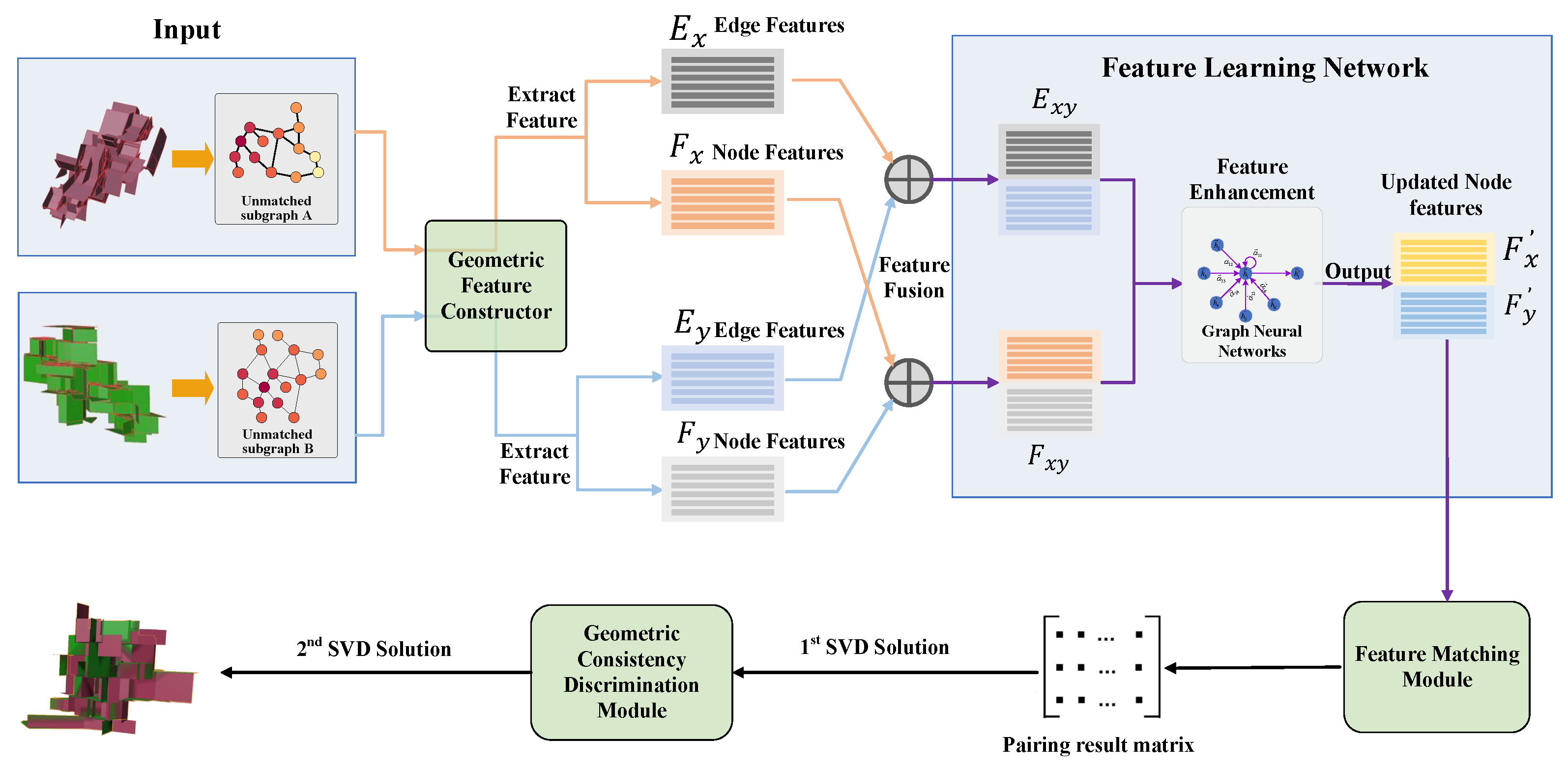
Given two geometric point clouds with coordinates, denoted as ${\displaystyle V_{\mathrm{src}}=\{{\mathbf{x}}_1,\dots ,{\mathbf{x}}_n\}\in {\mathbb{R}}^3}$ and ${\displaystyle V_{\mathrm{tgt}}=\{{\mathbf{y}}_1,\dots ,{\mathbf{y}}_n\}\in {\mathbb{R}}^3}$, and their corresponding edge relationships ${\displaystyle E_{\mathrm{src}}=\{{\mathbf{e}}_{x1},\dots ,{\mathbf{e}}_{xn}\}\in {\mathbb{R}}^2}$ and ${\displaystyle E_{\mathrm{tgt}}=\{{\mathbf{e}}_{y1},\dots ,{\mathbf{e}}_{yn}\}\in {\mathbb{R}}^2}$, our goal is to align the source graph structures with the target graph structure within the same coordinate system through rigid rotation (${\displaystyle \mathbf{R}}$) and translation (${\displaystyle \mathbf{T}}$). Ideally, the points in the graph structures correspond to each other and can be represented by the following equation:

$${\mathbf{y}}_i=\mathbf{R}{\mathbf{x}}_i+\mathbf{T}+{\mathbf{N}}_i$$

(1)

where ${\displaystyle {\mathbf{N}}_i}$ is the noise vector. The objective is to compute the rotation and translation matrices (${\displaystyle \mathbf{R}}$ and ${\displaystyle \mathbf{T}}$) to minimize the least-squares error:

$$\mathrm{error}(\mathbf{R},\mathbf{T})={\displaystyle \frac{1}{N}}\sum _{i=1}^N{\parallel \mathbf{R}{\mathbf{x}}_i+\mathbf{T}-{\mathbf{y}}_i\parallel }^2$$

(2)

However, during the registration process, the points in the two subgraphs do not correspond perfectly. Therefore, it is essential to employ specific methods to identify the corresponding points. In this paper, we utilize the existing point and edge information to predict the correspondence matrix ${\displaystyle {\mathbf{C}}_x\in {\mathbb{R}}^{|V_{\mathrm{src}}|\times |V_{\mathrm{tgt}}|}}$ through an end-to-end neural network. Once the correspondences are established, the rigid transformation parameters can be obtained using Singular Value Decomposition (SVD).

Given two partially overlapping geometric graph structures ${\displaystyle G_{\mathrm{src}}=(V_{\mathrm{src}},E_{\mathrm{src}})}$ and ${\displaystyle G_{\mathrm{tgt}}=(V_{\mathrm{tgt}},E_{\mathrm{tgt}})}$, where ${\displaystyle V=\{{\mathbf{x}}_i\in {\mathbb{R}}^3\}}$ represents the set of vertices and ${\displaystyle E=\{{\mathbf{e}}_{ij}\in {\mathbb{R}}^2\}}$ denotes the set of edges, the registration objective is to determine the rigid transformation (${\displaystyle \mathbf{R},\mathbf{T}}$) that minimizes the error as follows:

$$\mathrm{error}(\mathbf{R},\mathbf{T})={\displaystyle \frac{1}{N}}\sum _{i=1}^N{\parallel \mathbf{R}{\mathbf{x}}_i+\mathbf{T}-{\mathbf{y}}_{\pi \left(i\right)}\parallel }^2$$

(3)

where ${\displaystyle \pi \left(i\right):V_{\mathrm{src}}\to V_{\mathrm{tgt}}}$ denotes the point correspondence. After predicting the correspondence matrix ${\displaystyle {\mathbf{C}}_x}$ using an end-to-end neural network, the optimal transformation parameters are obtained via SVD.

4. Methods

The proposed graph structure registration framework, as shown in Figure 1, consists of four core modules: the Feature Construction Module (FCM), the Feature Learning Network Module (FLM), the Node Feature Matching Module (NFM), and the Geometric Consistency Discrimination Module (GCDM). The specific workflow is shown as follows:

For two geometric point cloud subgraphs with different poses and positions, the key point features and edge features are first extracted using the feature construction module. This module integrates geometric features and complex network indicators to generate 15-dimensional node feature vectors and 5-dimensional edge feature vectors. Subsequently, these features are fed into the designed EKNet graph neural network. It employs GraphKAN layers and EdgeConv layers to perform hierarchical feature aggregation, thereby enhancing the feature vectors of each point.

Next, based on a cosine similarity threshold, matching point pairs are filtered according to their feature vectors. The rotation and translation matrices are then solved using Singular Value Decomposition (SVD). Finally, through the Geometric Consistency Discrimination Module, the registration result is obtained after another round of SVD, aligning the point clouds into a unified coordinate system.

4.1. Feature Construction Module (FCM)

In graph neural networks, the number of nodes and edges is fixed, allowing for the construction of relevant features. This process serves as a means of data preprocessing and dimensionality reduction, thereby improving the accuracy and interpretability of model training and guiding models to learn more effective data representations. Subsequently, features are designed and extracted from the graph data of the geometric point clouds. For the graphs ${\displaystyle G_{\mathrm{src}}}$ and ${\displaystyle G_{\mathrm{tgt}}}$ to be registered, sorting is performed in the order of ${\displaystyle G_{\mathrm{src}1}}$, ${\displaystyle G_{\mathrm{tgt}1}}$, ${\displaystyle G_{\mathrm{src}2}}$, and ${\displaystyle G_{\mathrm{tgt}2}}$ to facilitate subsequent feature construction.

Node features are categorized into two main types: geometric features and complex network features. Geometric features, due to their intuitiveness, can effectively capture the geometric attributes of building structures and are computationally simple and efficient. Specifically, geometric features include degree, mean distance, minimum distance, maximum distance, mean angle, minimum angle, maximum angle, and mean orientation direction.

The calculation formulas for degree, mean distance, mean orientation, and mean angle are provided in

Table 1. Formula and meaning of geometric characteristics.

Feature	Formula	Meaning
Degree	${\displaystyle k_i=\sum _{j=1}^N{A}_{ij}}$	The number of edges connected to vertex ${\displaystyle i}$.
Average Distance	${\displaystyle L=\frac{1}{k_i}\sum _{i\ne j}{d}_{ij}}$	The average distance of the sum of the lengths of all edges where the point is located.
Average Orientation	${\displaystyle {\overrightarrow{v}}_{\mathrm{avg}}=\frac{1}{k_i}\sum _{i\ne j}{\overrightarrow{v}}_{ij}}$	The value obtained by normalizing the sum of vectors extending in the direction of all edges where the point is located, starting from that point.
Average Angles	${\displaystyle {\theta }_{av{g}_i}=\frac{2}{k_i(k_i-1)}\sum _{j=1}^N{\theta }_{ij}}$	The average degree of angle between the vectors that extend from this point to all the edges where the point is located, measured as the angle between each pair of vectors.

where the degree ${\displaystyle k_i}$ of each node is the number of connected edges of the vertex. ${\displaystyle A_{ij}}$ represents the adjacency matrix between nodes ${\displaystyle i}$ and ${\displaystyle j}$. ${\displaystyle d_{ij}}$ represents the distance between nodes ${\displaystyle i}$ and ${\displaystyle j}$. ${\displaystyle {\overrightarrow{v}}_{ij}}$ represents the vector formed between nodes ${\displaystyle i}$ and ${\displaystyle j}$. The average orientation vector includes dimensions along the three coordinate axes of xyz. ${\displaystyle {\theta }_{ij}}$ denotes the angle between node ${\displaystyle i}$ and the two edges it is connected to.

.

The characteristics of complex networks can reveal the essence and laws of the entire system and highlight several important key nodes in the geometric point cloud. The relevant formulas and meanings are presented as

Table 2. Complex network feature formulas and meanings.

Feature	Formula	Meaning
Clustering Coefficient	${\displaystyle C_i=\frac{2\parallel \{e_{jk}:v_j,v_k\in N_i,e_{jk}\in E\}\parallel }{k_i(k_i-1)}}$	The coefficient of the degree of clustering between vertices in a graph.
Degree Centrality	${\displaystyle C_D\left(v\right)=\frac{k_i}{N-1}}$	The degree to which a node is connected to all other nodes.
Eigenvector Centrality	${\displaystyle C_E\left(v\right)=\frac{1}{\lambda }\sum _{u\in N\left(v\right)}{C}_E\left(u\right)}$	Ranking of the likelihood of a node being visited during an infinite-length random walk in the graph.
PageRank	${\displaystyle PR{\left(a\right)}_{i+1}=\sum _{i=0}^n\frac{PR{\left(T_i\right)}_i}{L\left(T_i\right)}}$	Measures the importance of nodes through random walk models and transition probability matrices.
Load Centrality	${\displaystyle C_L\left(v\right)=\sum _{s\ne v\ne t\in V}\frac{{\sigma }_{st}\left(v\right)}{{\sigma }_{st}}}$	Calculates the proportion of all shortest paths in the network that pass through this node.

where ${\displaystyle k_i}$ denotes the degree of node ${\displaystyle i}$, and ${\displaystyle N_i}$ represents the set of neighboring nodes of node ${\displaystyle i}$. ${\displaystyle C_E\left(u\right)}$ indicates the Eigenvector Centrality of neighboring node ${\displaystyle u}$. ${\displaystyle E_{jk}}$ represents the edge connecting nodes ${\displaystyle v_j}$ and ${\displaystyle v_k}$; ${\displaystyle N_i}$ represents the set of neighboring nodes of node ${\displaystyle v_i}$. ${\displaystyle E}$ represents the set of edges in the graph. ${\displaystyle C_E\left(v\right)}$ indicates the Eigenvector Centrality of node ${\displaystyle v}$, and ${\displaystyle N\left(v\right)}$ denotes the set of neighboring nodes of node ${\displaystyle v}$. ${\displaystyle \lambda }$ is a constant (eigenvalue). ${\displaystyle PR\left(T_i\right)}$ refers to the PageRank values of other nodes pointing to node ${\displaystyle a}$, and ${\displaystyle L\left(T_i\right)}$ represents the number of outgoing links from other nodes pointing to node ${\displaystyle a}$. The index ${\displaystyle i}$ indicates the iteration count. ${\displaystyle {\sigma }_{st}}$ is the total number of shortest paths from node ${\displaystyle s}$ to node ${\displaystyle t}$, and ${\displaystyle {\sigma }_{st}\left(v\right)}$ is the number of shortest paths passing through node ${\displaystyle v}$.

:

Based on these definitions, a 15-dimensional feature vector is constructed. Finally, all features are normalized to ensure consistency and comparability.

For edge features, we similarly designed several important edge attributes, including the following:

• Edge length: The Euclidean distance between the two endpoints of the edge.
• Edge direction: The normalized direction vector from one endpoint to the other (3 dimensions including xyz).
• Edge loop count: The number of loops occupied by an edge. The meaning of a ring is to characterize the number of connected edges that are connected head to tail to form a closed loop.

These features collectively form a five-dimensional edge feature vector. This helps in understanding the structure and layout of objects. Finally, the edge features are also normalized.

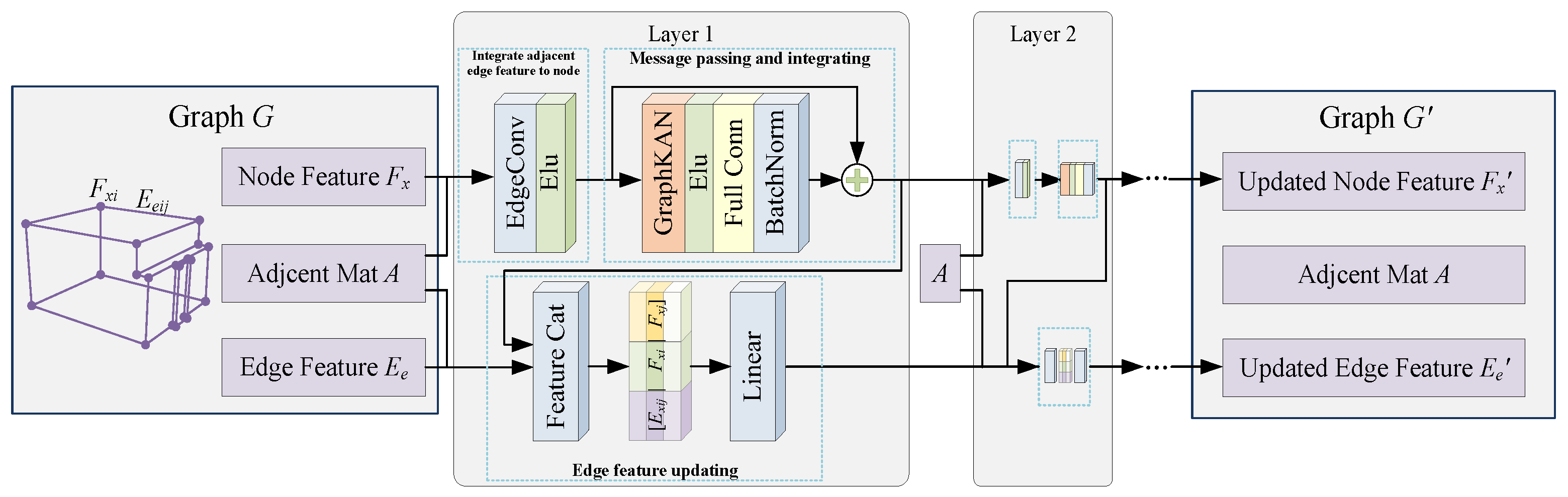
4.2. Feature Learning Network Module (FLNM)

After obtaining the node and edge features for each graph, this study proposes a novel graph neural network architecture, named EKNet, to further extract features from the geometric point cloud graphs. EKNet aims to enhance computational efficiency while maintaining accuracy, addressing the issues of high computational cost and excessive parameters in other graph neural networks.

Figure 2 illustrates the overall structure of EKNet. The network is designed to efficiently process geometric point cloud data by integrating specialized layers that capture both local and global features. This architecture ensures that EKNet can handle large-scale point clouds with reduced computational overhead compared to existing methods.

4.2.1. Update of Node Features

To enhance the accuracy of graph structure registration while reducing computational costs and improving efficiency, we propose a novel graph neural network architecture, namely EKNet. The network framework we designed mainly consists of two layers of graph neural networks: an KAN layer and EdgeConv layer. When the node features pass through each layer of the graph neural network, they will be aggregated and updated in sequence. This process strengthens the global feature representation capabilities of nodes, edges, and the entire graph, thereby laying a solid foundation for the subsequent feature matching stage. Subsequently, these features are processed through an EdgeConv layer and GraphKAN layer. The EdgeConv layer, derived from the Dynamic Graph CNN (DGCNN) [48], primarily addresses the issue that networks such as PointNet [37] fail to fully consider the geometric structure relationships in local information when extracting node features. By constructing a local neighborhood graph and applying convolution-like operations on edges between adjacent point pairs to develop local geometric structures, its dynamic graph updating method enables the network to better capture the local geometric information of point clouds, thereby improving the accuracy of point cloud registration. We design the output feature dimension to be 64. The specific process is as follows:

Since the feature extraction process of the two subgraphs is the same, one of the subgraphs is taken as an example. Firstly, take the initial node features ${\displaystyle F_x}$ and adjacency matrix after geometrization as inputs. Then, construct a directed graph ${\displaystyle G}$ as the ${\displaystyle k}$-nearest neighbor (${\displaystyle k}$-NN) graph of ${\displaystyle x}$ in ${\displaystyle {\mathbb{R}}^F}$. The graph includes self-loops, meaning that each node also points to itself. Define the edge features of the paired subgraphs as ${\displaystyle E_{x_{ij}}=h_{\Theta }(x_i,x_j)}$, where ${\displaystyle h_{\Theta }:{\mathbb{R}}^F\times {\mathbb{R}}^F\to {\mathbb{R}}^{F^{\prime }}}$ is a nonlinear function with a set of learnable parameters ${\displaystyle \Theta }$. Here, ${\displaystyle F}$ is 15-dimensional, and ${\displaystyle F^{\prime }}$ is 64-dimensional.

The processing of features in graph neural networks typically involves two steps: (a) Aggregation. The message function aims to combine the adjacent features of the target node, including its own features, the features of neighboring nodes, and the edge features connecting to neighboring nodes, into a single vector. This vector will represent the neighborhood information of the central node. (b) Update. The node update function is employed to integrate the node features of the current layer with the messages obtained through the message passing function, thereby updating the node features of the next graph layer.

(a) EdgeConv Layer

The EdgeConv layer employs an asymmetric edge feature calculation function. It explicitly combines global shape structures with local neighborhood information. The aggregation function ${\displaystyle h_{\Theta }}$ is represented as

$$h_{\Theta }(x_i,x_j)=h_{\Theta }(x_i,x_j-x_i)$$

(4)

where ${\displaystyle h_{\Theta }}$ integrates the global shape structure encapsulated by the central coordinate ${\displaystyle x_i}$ and the local proximity data represented by ${\displaystyle x_j-x_i}$. Then it is fed into another perceptron to obtain the features. The specific formula for the ${\displaystyle m}$-th channel is given by

$$E_{x_{ijm}}^{\prime }=\mathrm{ReLU}({\theta }_m·(x_j-x_i)+{\varphi }_m·x_i)$$

(5)

where ${\displaystyle \theta =({\theta }_1,\dots ,{\theta }_m,{\varphi }_1,\dots ,{\varphi }_m)}$ denotes the learnable parameters. The m-th channel represents the m-th dimension of the feature vector. In multi-channel feature representation, each channel can capture distinct feature information. ReLU stands for the Rectified Linear Unit function. The aggregation function is applied to update the values of the ${\displaystyle m}$-th channels of node ${\displaystyle i}$:

$$x_{im}^{\prime }=\underset{j:(i,j)\in E}{max}{E}_{x_{ijm}}^{\prime }$$

(6)

where m-channels denote the m-th dimension in the feature vector. In multi-channel feature representation, each channel can capture different feature information.

Despite its advantages, the EdgeConv layer has several limitations. It relies on a transformation network to offset nodes, which increases the network’s size. Additionally, the deep features and their neighbors may be too similar to provide valuable edge vectors. Moreover, EdgeConv has many trainable parameters, making it difficult to find the optimal parameters during network training, especially for large-scale building data, resulting in slower processing speeds. While EdgeConv considers the coordinates of points and the distances to neighboring points, it neglects the vector directions between adjacent points, leading to a partial loss of local geometric information. Therefore, relying solely on the EdgeConv layer is insufficient.

After the EdgeConv layer, the features are passed through an ELU (Exponential Linear Unit) activation function [49]. Compared to ReLU, ELU has negative values, which push the mean activations closer to zero. This speeds up learning because it brings the gradient closer to the natural gradient, reducing the bias shift effect.

(b) GraphKAN

Inspired by Zhang [50], Kolmogorov–Arnold Networks (KANs) are applied to graph neural networks (GNNs) to replace traditional multi-layer perceptrons (MLPs) and activation functions [51]. This approach enhances nonlinearity and representation capabilities by using spline-based univariate functions as learnable activation functions. It improves model efficiency and interpretability, addresses information loss issues, and enhances performance across different datasets. The content of this theorem is that any multivariate continuous function ${\displaystyle f(x_1,\dots ,x_n)}$ on a bounded domain can be expressed as a finite combination of simpler one-dimensional continuous functions. The formula can be expressed as follows:

$$f(x_1,\dots ,x_n)=\sum _{q=1}^{2n+1}{\Phi }_q\left(\sum _{p=1}^n{\varphi }_{q,p}\left(x_p\right)\right),$$

(7)

where ${\displaystyle {\varphi }_{q,p}}$ maps the interval ${\displaystyle [0,1]}$ to ${\displaystyle \mathbb{R}}$, and ${\displaystyle {\Phi }_q}$ performs a mapping from ${\displaystyle \mathbb{R}\to \mathbb{R}}$. However, these one-dimensional mappings can exhibit irregularities and even fractal properties, making them challenging to learn in real-world applications.

Specifically, the Kolmogorov–Arnold Network (KAN) can be formulated as

$$x_{l+1}={\Phi }_l{x}_l,$$

(8)

where ${\displaystyle {\Phi }_l}$ denotes the following matrix:

$${\Phi }_l=\left(\begin{array}{cccc}{\varphi }_{1,1}& {\varphi }_{1,2}& \dots & {\varphi }_{1,n}\\ {\varphi }_{2,1}& {\varphi }_{2,2}& \dots & {\varphi }_{2,n}\\ ⋮& ⋮& \ddots & ⋮\\ {\varphi }_{m,1}& {\varphi }_{m,2}& \dots & {\varphi }_{m,n}\end{array}\right).$$

(9)

Since geometric graph structures belong to non-Euclidean space data, where the set of neighboring nodes for each node is dynamically changing, graph neural networks (GNNs) can leverage the message passing mechanism to propagate and update node and edge features within the graph, adapting to different topological structures.

For the aggregation process, in the propagation at layer ${\displaystyle t}$, it includes the node’s own feature ${\displaystyle h_v^t}$, the features of neighboring nodes ${\displaystyle h_w^t}$, and the edge features ${\displaystyle e_{vw}^t}$ connecting to neighboring nodes. This aggregation forms the message vector ${\displaystyle m}$, which is then passed to the target node. The formula is presented as

$$m_v^{t+1}=\sum _{w\in N\left(v\right)}{M}^t\left(h_v^t,h_w^t,e_{vw}^t\right)$$

(10)

where ${\displaystyle m_v^{t+1}}$ represents the aggregated data received by node ${\displaystyle v}$ at layer ${\displaystyle t+1}$. The function ${\displaystyle M^t}$ is responsible for the message passing mechanism. In the current layer ${\displaystyle t}$, the feature of node ${\displaystyle v}$ is denoted by ${\displaystyle h_v^t}$. The set of neighboring nodes connected to node ${\displaystyle v}$ is denoted by ${\displaystyle N\left(v\right)}$. Additionally, ${\displaystyle h_w^t}$ represents the features of these neighboring nodes in the same layer. Moreover, ${\displaystyle e_{vw}^t}$ captures the attribute information of the edge from node ${\displaystyle v}$ to node ${\displaystyle w}$. The formula for the update progress is depicted as follows:

$$h_v^{t+1}=U^t\left(h_v^t,m_v^{t+1}\right)$$

(11)

where ${\displaystyle U^t}$ is the node update function at layer ${\displaystyle t}$, which takes the current node state and the received messages as inputs and generates the new node state.

Compared to EdgeConv, which primarily focuses on local neighborhood node features, GraphKAN can more effectively capture global graph structure information through the introduction of attention mechanisms and graph kernels, thereby enhancing registration performance. Additionally, EdgeConv is sensitive to changes in node degrees within the graph structure and is prone to being affected by noise or outlier nodes. In contrast, GraphKAN leverages nuclear norm regularization and attention mechanisms to enhance the robustness of registration, showing greater tolerance to degree changes and noise. Moreover, GraphKAN can effectively identify complex relationships between nodes, further improving registration accuracy. When dealing with sparse graphs, EdgeConv may lead to over-smoothing issues, while GraphKAN, through attention mechanisms and nuclear norm regularization, better maintains the distinguishability between nodes, more effectively addressing the registration problem of sparse graphs. Therefore, the combination of GraphKAN and EdgeConv can significantly improve registration accuracy.

However, GraphKAN also has some limitations. Due to the complex structure of GraphKAN, it may have a relatively long training cycle and high computational costs. To meet the needs of building structure registration, this study adopts a single-layer network design, increasing the feature vector dimension from 64 to 128 to reduce operational demands and costs.

Subsequently, fully connected layers are added, and residual connections and normalization layers are employed to stabilize the training process, enhancing the model’s expressive power and performance to extract more complex graph structure information. This approach facilitates easier convergence during model training, effectively reducing training time and computational resource consumption.

4.2.2. Update of Edge Features

Inspired by the work of Zhou et al. [52], we adopt a novel feature update method that can simultaneously aggregate neighbor node information and multidimensional edge features to the central node. After the node feature update is completed, the updated node features are concatenated with the edge features to update the edge feature information. In each layer, node features not only aggregate part of the initial features but also integrate features from the previous layer, effectively avoiding the problem of feature oversmoothing. This method has three significant characteristics:

• It can obtain non-local structural features of nodes as well as more refined higher-order features.
• It can effectively prevent the problem of feature oversmoothing.
• It can aggregate multidimensional edge features to the central node.

Through the above process, a round of node updates in the graph structure is completed.

4.3. Loss Function

We employ a cosine similarity-based loss function to measure the similarity between feature vectors. For a batch of data ${\displaystyle D(a,b,y)}$ containing ${\displaystyle N}$ samples, where ${\displaystyle a}$ and ${\displaystyle b}$ represent the feature vectors of two nodes output by the neural network, and ${\displaystyle y}$ denotes the true label of the point cloud pair (taking values in ${\displaystyle \{1,-1\}}$ to indicate similarity and dissimilarity, respectively), the loss function for the ${\displaystyle i}$-th sample is expressed as follows:

$${\mathrm{loss}}_i=\left\{\begin{array}{cc}1-cos(a_i,b_i),\hfill & \mathrm{if}{y}_i=1,\hfill \\ max(0,cos(a_i,b_i)-\mathrm{margin}),\hfill & \mathrm{if}{y}_i=-1,\hfill \end{array}\right.$$

(12)

where ${\displaystyle cos(a_i,b_i)}$ denotes the cosine similarity between the feature vectors ${\displaystyle a_i}$ and ${\displaystyle b_i}$ of sample ${\displaystyle i}$, and ${\displaystyle \mathrm{margin}}$ is a predefined margin value set to 0.4.

The network outputs feature vectors of matched point pairs, with an equal number of positive and negative pairs extracted. The feature similarity between these pairs is computed, and the labels for negative pairs are set to ${\displaystyle -}$1, while positive pairs have labels of 1. Given that the number of negative samples far exceeds that of positive samples, we set the ratio of positive to negative samples to 1:8 to improve training effectiveness. Subsequently, the total loss function is obtained by weighted summation based on the total number of positive and negative samples. The weighted loss function is specified as follows:

$$\mathrm{Loss}={\mathrm{Loss}}_{\mathrm{pos}}·{\displaystyle \frac{{\sum }_{i=1}^n{X}_{\mathrm{label},i}}{N}}+{\mathrm{Loss}}_{\mathrm{neg}}·{\displaystyle \frac{{\sum }_{i=1}^n{X}_{\mathrm{mis},i}}{N}},$$

(13)

where ${\displaystyle {\mathrm{Loss}}_{\mathrm{pos}}}$ represents the cross-entropy loss function for positive samples, and ${\displaystyle X_{\mathrm{label},i}}$ denotes a pair of labels. Conversely, ${\displaystyle {\mathrm{Loss}}_{\mathrm{neg}}}$ indicates the cross-entropy loss function for negative pairs, and ${\displaystyle X_{\mathrm{mis},i}}$ represents a pair of mislabeled point clouds.

The design of this loss function is simple and easy to optimize, focusing on the directional differences between two feature vectors rather than their specific numerical values. This approach is particularly effective in handling class imbalance problems. Additionally, the loss function is applicable to high-dimensional data, mitigating the impact of dimensionality and thereby enhancing the model’s accuracy and robustness.

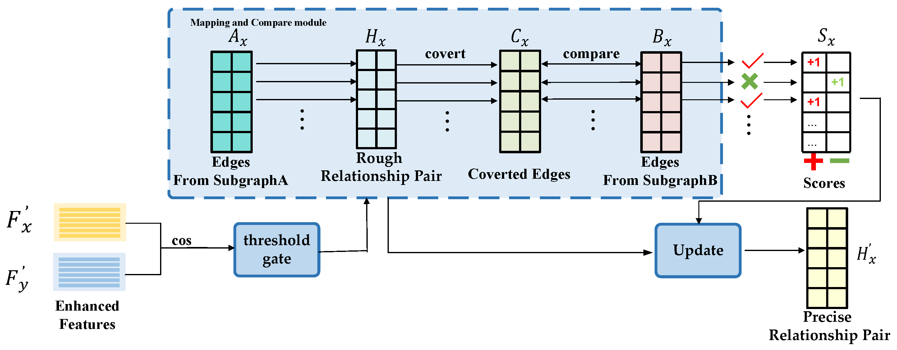
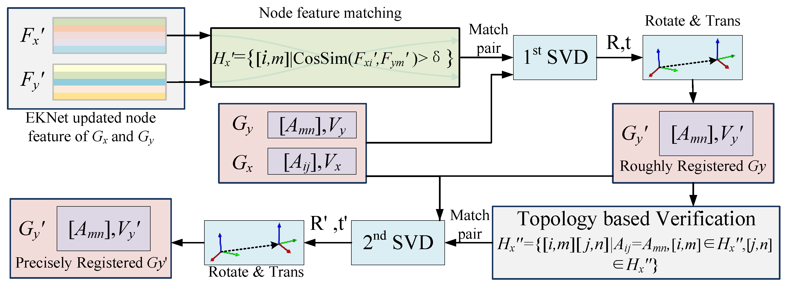
4.4. Node Feature Matching Module (NFMM)

To address the issue of non-matching point pairs that may arise after network training, we design a Node Feature Matching Module (NFMM). This module aims to identify and exclude mismatched point pairs. The specific steps are detailed as follows:

• Threshold Setting: The module begins by computing the cosine similarity matrix from the enhanced node features of the corresponding points in the two images. A threshold filter is then applied, which considers pairs with a cosine similarity below 0.8 as non-matching and excludes them. The pairs with the highest cosine values are selected to form a preliminary coarse correspondence matrix ${\displaystyle H_x}$.
• Prediction Matrix Generation: We map each edge from the edge matrix ${\displaystyle A_x}$ of one of the images to be registered, based on the point correspondence matrix ${\displaystyle H_x}$, by scanning ${\displaystyle A_x}$ row by row. This process results in the predicted point correspondence matrix ${\displaystyle C_x}$ for the target image.
• Accumulation Matrix Construction: An accumulation matrix ${\displaystyle S_x}$ is constructed to match the generated edge correspondences. The first column of ${\displaystyle S_x}$ represents the positive accumulation for each point, while the second column represents the negative accumulation.
• Comparison: Matrix ${\displaystyle C_x}$ is compared row by row with the edge distance matrix ${\displaystyle B_x}$ of the corresponding image to be registered. If an edge from ${\displaystyle C_x}$ is found in ${\displaystyle B_x}$, the positive integral for the corresponding points in the integral matrix ${\displaystyle S_x}$ is incremented by one; otherwise, the negative integral is incremented.
• Updating the Correspondence Matrix: After completing the comparison of all edges, the integral matrix ${\displaystyle S_x}$ is used to determine the retention of edges. An edge is retained if the absolute value of its positive integral exceeds its negative integral; otherwise, it is discarded. The final output is the feature-matched point cloud correspondence matrix ${\displaystyle H_x^{\prime }}$.

The algorithm module is described as Figure 3:

4.5. Geometric Consistency Discrimination Module (GCDM)

Initially, a coarse registration process is performed in this study. Given the point correspondence matrix ${\displaystyle H_x^{\prime }}$ output by the feature matching module, the preliminary rotation matrix ${\displaystyle \mathbf{R}}$ and translation vector ${\displaystyle \mathbf{T}}$ are solved using Singular Value Decomposition (SVD).

Subsequently, the Geometric Consistency Discrimination Module (GCDM) is deployed to validate the coarse registration results. Based on the premise that the translation distance of each point should theoretically remain consistent during the registration process, the coarse registration results are analyzed. Specifically, the frequency distribution of translation errors for the registered keypoints in the ${\displaystyle x}$, ${\displaystyle y}$, and ${\displaystyle z}$ directions is statistically analyzed, and points that fall within the concentrated error distribution intervals in all three directions are identified. These point pairs are considered correctly registered pairs. Subsequently, another round of SVD is performed on these correctly registered pairs to obtain the final rotation matrix ${\displaystyle \mathbf{R}}$ and translation vector ${\displaystyle \mathbf{T}}$. Finally, the transformation and restoration of Gy are achieved through this process, as shown in Figure 4. The colored arrows in the figure indicate the schematic diagram of the Cartesian coordinate system of the two subfigures.

Through the above steps, the Geometric Consistency Discrimination Module effectively enhances the accuracy of registration, ensuring that the final registration results maintain geometric consistency. This process strengthens the robustness and reliability of the model.

5. Experiments

In this section, we demonstrate the robustness and effectiveness of our algorithm under different noise levels and overlap rates by conducting registration experiments on a self-built point cloud geometric dataset.

5.1. Dataset Construction

Currently, there is a lack of publicly available datasets for geometric point clouds. To simulate building structure data and facilitate the training of graph neural networks, we first constructed a graph-structured dataset with building structure characteristics. The geometric building structures are composed of interconnected planes. In the Cartesian coordinate system, a base plane with ${\displaystyle z=0}$ is first constructed, consisting of seven randomly generated points with ${\displaystyle z=0}$. Since most buildings have horizontal and vertical structures, new planes are added in these directions. Each time, an existing plane is selected probabilistically as a reference plane. If the reference plane is horizontal, two points are randomly selected from this plane to form the base edge of a rectangle, and the height of the rectangle is randomly sampled to construct a vertical plane. If the reference plane is vertical, either the top or bottom edge is chosen as the reference edge ${\displaystyle E_{\mathrm{ref}}}$. Within a horizontal plane centered at the midpoint of ${\displaystyle E_{\mathrm{ref}}}$ with a radius of 3 m, ${\displaystyle n=10}$ points are randomly added, and only those on the side with more points relative to ${\displaystyle E_{\mathrm{ref}}}$ are retained. A new horizontal plane is constructed based on the remaining points and the endpoints of ${\displaystyle E_{\mathrm{ref}}}$ by computing the convex hull. To form an expanding trend horizontally and vertically, new planes are given a higher sampling probability when selecting reference planes. This process is repeated until a sufficient number of planes are generated. Since all planes are generated based on existing edges, the resulting interconnected structure forms a graph ${\displaystyle G}$.

To construct subgraphs with different overlap rates, we extend new graphs from a base graph that already has a certain number of planes. The common base represents the overlapping part between different new graphs. By applying random rotations, translations, and positional noise to nodes, data under various conditions can be simulated.

In total, 1000 pairs of graph data were generated for model training and verification, thereby forming a dataset GPCR.

5.2. Evaluation Metrics

To analyze and compare our results with previous algorithms on the same scale, we selected five commonly used evaluation criteria for point cloud registration algorithms: the root mean square error (RMSE) and mean absolute error (MAE) of the rotation Euler angles and translation vectors. The time metric represents the duration required to obtain the output feature vectors using the respective network method on the test set. Let the true rotation matrix ${\displaystyle \mathbf{R}}$ be represented by the Euler angles ${\displaystyle {\mathrm{Eu}}_{\mathrm{gt}}}$, and the predicted rotation matrix ${\displaystyle \mathbf{R}}$ by ${\displaystyle {\mathrm{Eu}}_{\mathrm{pre}}}$. The rotation error is calculated as follows:

$$\mathrm{RMSE}\left(\mathbf{R}\right)=\sqrt{{\displaystyle \frac{1}{n}}\sum _{i=1}^n{({\mathrm{Eu}}_{\mathrm{pre}}-{\mathrm{Eu}}_{\mathrm{gt}})}^2},$$

(14)

$$\mathrm{MAE}\left(\mathbf{R}\right)={\displaystyle \frac{1}{n}}\sum _{i=1}^n|{\mathrm{Eu}}_{\mathrm{pre}}-{\mathrm{Eu}}_{\mathrm{gt}}|.$$

(15)

For the translation vector error, ${\displaystyle {\mathbf{t}}_{\mathrm{pre}}}$ is the predicted translation vector, and ${\displaystyle {\mathbf{t}}_{\mathrm{gt}}}$ is the true translation vector. The translation error is calculated as follows:

$$\mathrm{RMSE}\left(\mathbf{t}\right)=\sqrt{{\displaystyle \frac{1}{n}}\sum _{i=1}^n{({\mathbf{t}}_{\mathrm{pre}}-{\mathbf{t}}_{\mathrm{gt}})}^2},$$

(16)

$$\mathrm{MAE}\left(\mathbf{t}\right)={\displaystyle \frac{1}{n}}\sum _{i=1}^n|{\mathbf{t}}_{\mathrm{pre}}-{\mathbf{t}}_{\mathrm{gt}}|.$$

(17)

5.3. Implementation Details

To comprehensively evaluate the algorithm’s performance, experiments were conducted to verify the impact of three key factors on registration results: the noise level of graph nodes, the difference in initial translation and rotation angles, and the overlap rate between the graphs to be registered.

First, a noise-free clean dataset was constructed. Using the aforementioned method, graph structures of simulated buildings were generated, and subgraphs with overlap rates of 20%, 40%, and 60% were set. Subsequently, these graphs were subjected to random rotations and translations. For the initial parameter settings, the random translation range in each direction was set to ${\displaystyle [-10,10]}$ meters, and the rotation angle range was set to ${\displaystyle [-\pi ,\pi ]}$, thereby generating the rotation matrix ${\displaystyle \mathbf{R}}$ and translation vector ${\displaystyle \mathbf{T}}$. A total of 1000 graphs ${\displaystyle G_{tgt}}$ to be registered were generated. Based on the 60% clean data, point cloud data with Gaussian noise were further constructed. Normal distribution noise with a mean of 0 and a standard deviation of 1 was added to the clean data to simulate positional changes of each point in real-world scenarios.

Our model was run on an NVIDIA GeForce RTX 4090 (NVIDIA, Santa Clara, CA, USA) and implemented within the PyTorch 2.3.1 framework, with 100 training epochs. The Adam optimizer was used with an initial learning rate of 0.001. Training was performed using random sampling, and the dataset was split into training, validation, and test sets in an 8:1:1 ratio. Since conventional point cloud registration techniques are mainly applied in scenarios featuring large-scale data and dense point clouds, and they either do not utilize edge information or rely on image-based point cloud data, we opt for the graph neural network approach for comparison to ensure a fairer benchmarking. We compared our method with several state-of-the-art algorithms, including Graph Convolutional Network (GCN) [21], Graph Attention Network (GAT) [44], and three other learning-based methods: GDC [53], GraphKAN [50], SGC [54], and NIGCN [55]. For the comparison methods, we used the code provided by the authors and trained the models according to the settings specified by the authors. The input and output of the networks were set to be the entire concatenated graph, consistent with our method. All networks were retrained from scratch, as pre-trained models were not available.

Through these detailed experimental settings, the algorithm’s performance can be comprehensively evaluated under different noise levels, initial rotation angles, and overlap rates.

5.4. Experimental Results

Compared with conventional point cloud registration methods, this study improves the registration process by incorporating edge information. Given the difficulty in directly comparing with all existing methods comprehensively, several graph neural network methods were selected for comparative experiments, with other modules kept unchanged.

5.4.1. Comparison Experiments with Different Overlap Rates

First, comparative experiments were conducted on noise-free data with initial structure overlap rates of 20%, 40%, and 60%. The test set contained 100 pairs of graphs. The registration results are shown in

Table 3. Registration performance at 20% overlap.

Method	RMSE(R)	RMSE(t)	MAE(R)	MAE(t)	Times(s)
GDC [53]	0.158	1.080	0.085	0.554	17.8
GAT [44]	0.245	1.673	0.144	0.937	168.3
GCN [21]	0.176	1.238	0.092	0.610	17.4
GraphKan [50]	0.103	0.719	0.054	0.349	20.2
SGC [54]	0.451	3.286	0.280	1.971	21.9
NIGCN [55]	0.368	2.713	0.233	1.664	30.5
Ours	0.030	0.193	0.010	0.067	12.7

,

Table 4. Registration performance at 40% overlap.

Method	RMSE(R)	RMSE(t)	MAE(R)	MAE(t)	Times(s)
GDC [53]	0.051	0.302	0.018	0.126	17.5
GAT [44]	0.104	0.909	0.036	0.273	168.4
GCN [21]	0.045	0.316	0.011	0.074	21.9
GraphKan [50]	0.023	0.173	0.011	0.083	24.2
SGC [54]	0.244	1.842	0.116	0.855	27.8
NIGCN [55]	0.126	1.043	0.066	0.513	28.1
Ours	0.005	0.037	0.002	0.017	18.8

and

Table 5. Registration performance at 60% overlap.

Method	RMSE(R)	RMSE(t)	MAE(R)	MAE(t)	Times(s)
GDC [53]	0.012	0.083	0.006	0.046	19.4
GAT [44]	0.040	0.281	0.010	0.073	165.0
GCN [21]	0.014	0.100	0.007	0.057	19.1
GraphKan [50]	0.005	0.046	0.003	0.023	27.2
SGC [54]	0.086	0.592	0.031	0.237	28.6
NIGCN [55]	0.030	0.239	0.017	0.144	33.9
Ours	0.002	0.013	0.001	0.006	19.5

, demonstrating the performance comparison between our method and other similar methods. The experimental results indicate that our method achieved the best performance, surpassing other comparative methods.

Our method was compared with several traditional and popular graph neural network algorithms. The experimental results demonstrate that EKNet outperforms other graph neural learning-based algorithms across multiple metrics. Specifically, our algorithm achieves a Mean Squared Error (MSE) in Euler angle rotation that is two orders of magnitude lower than the commonly used GCN algorithm and one order of magnitude lower than the second-best GraphKAN method, resulting in a 94.98% improvement. The unit related to translation error is meters. In terms of translation vector error MSE(t), EKNet significantly outperforms the SGC algorithm and is one order of magnitude better than the GDC algorithm. EKNet requires a floating-point operation volume of 171.50 M and has a parameter count of only 3.166 K.

This significant performance improvement is primarily attributed to the feature construction module, which accurately extracts features, and the node feature matching module, which plays a crucial role in the registration process.

From the tables above, it is evident that there are significant differences in registration time among different algorithms. For example, the GAT algorithm, due to its high computational complexity, runs slowly, requiring 164 s to register 100 pairs of graphs with an overlap rate of 60%. In contrast, the GCN algorithm, with its simpler structure, runs faster but does not achieve the best registration results. Moreover, as the overlap rate decreases, the error increases for all methods, further demonstrating the advantage of our feature construction module in extracting precise features and the importance of the node feature matching module in the registration process.

The experimental results prove that EKNet can effectively handle the registration of partially overlapping point clouds and outperforms some popular registration algorithms in terms of performance.

5.4.2. Comparison Experiments with Noisy Data

To evaluate the robustness of different algorithms under noisy conditions, Gaussian noise with a mean of 0 and a standard deviation of 0.05 was added to each point in the graph-structured data with a 60% overlap rate. The other experimental conditions remained consistent with the previous experiments. The comparison results are shown in

Table 6. Registration performance at 60% overlap.

Method	RMSE(R)	RMSE(t)	MAE(R)	MAE(t)	Times(s)
GDC [53]	0.013	0.105	0.007	0.059	21.2
GAT [44]	0.051	0.451	0.012	0.092	165.5
GCN [21]	0.017	0.133	0.009	0.075	17.7
GraphKan [50]	0.008	0.060	0.004	0.033	23.5
SGC [54]	0.110	0.880	0.040	0.299	21.5
NIGCN [55]	0.117	0.943	0.043	0.320	26.1
Ours	0.003	0.021	0.002	0.014	18.8

.

We observed that the introduction of moderate noise led to a slight decrease in the overall rotation matrix error (MSE(R)) and translation vector error (MSE(t)), with minimal impact on the network’s running speed on the test set, demonstrating a certain level of interference resistance. Moreover, our algorithm was able to more effectively adapt to the registration task under high-noise conditions. Specifically, the NIGCN algorithm struggled to complete registration quickly and accurately under high-noise conditions. This is because noise points further disrupted the global consistency it relies on, failing to meet the registration process’s demands for global consistency and smoothness. In contrast, our deep learning-based registration algorithm could extract deeper-level features, effectively addressing this issue. In terms of running time, our algorithm and the GCN algorithm both achieved times around 18 s, showing high efficiency and significantly outperforming the GAT algorithm. However, the error of GCN’s method is only achieved with the support of other modules in our method, and it is still larger than ours. Therefore, compared with other registration algorithms, our algorithm demonstrated advantages in both high-noise conditions and running speed.

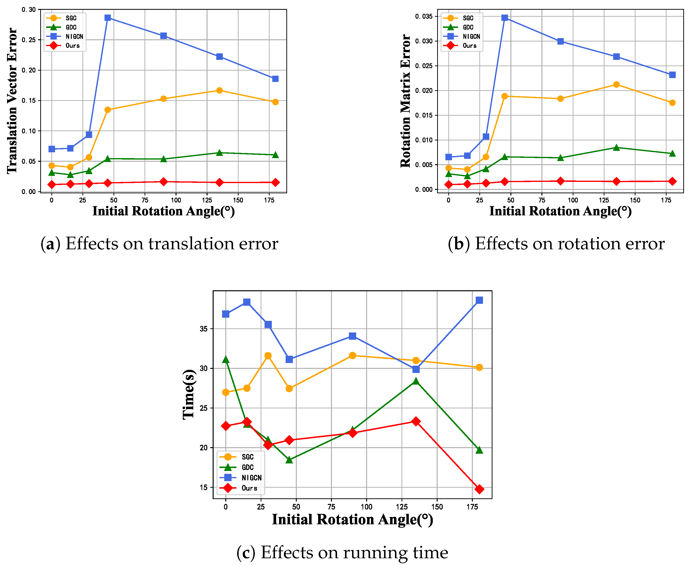
5.4.3. Effect of Initial Rotation Angles on Registration Results

To further analyze and validate the effectiveness and robustness of our algorithm, experiments with different initial rotation angles were conducted on the noisy dataset with a fixed overlap rate of 60%. In the experiments, the initial translation vector was kept constant at ${\displaystyle [-5,5]}$, while the initial rotation angles were systematically varied from [−0°,0°] to [−180°,180°] to explore the relationship between registration results and initial rotation angles. The experimental results are shown in Figure 5.

It can be observed that our algorithm exhibits high stability when the initial rotation angles are within the range of [0°,30°]. The rotation and translation errors significantly increase when the initial rotation angle reaches 30° or larger. However, after the initial rotation angle exceeds 90°, the errors of all algorithms begin to decrease. This phenomenon can be attributed to the fact that larger rotation angles make the features more distinct, facilitating the registration process.

Additionally, we found that the time required for algorithm output is not strongly correlated with the initial rotation angle. In contrast, the NIGCN algorithm shows insufficient stability and struggles to work effectively under large initial rotation angles, taking the longest time. This indicates that the NIGCN algorithm has difficulty achieving accurate registration when dealing with complex structures. Compared with SGC, GDC, and NIGCN algorithms, our algorithm demonstrates higher stability and robustness. Even under large initial rotation angles, our algorithm still provides stable and accurate registration results, with lower rotation and translation errors than other methods.

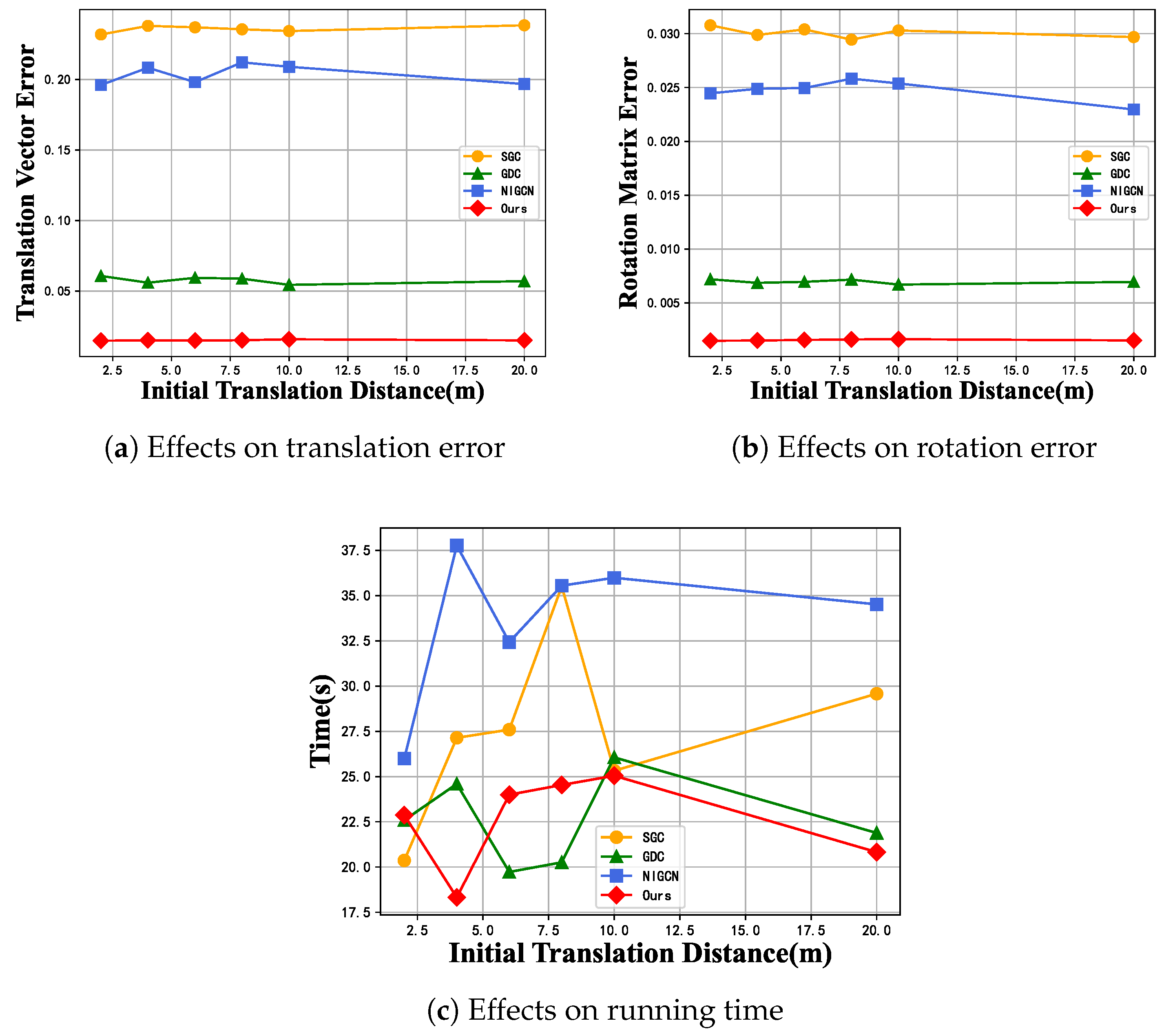
5.4.4. Effect of Initial Translation Distances on Registration Results

In this experiment, the initial rotation angles were fixed at [−90°,90°], and the initial translation distances were systematically varied from ${\displaystyle [-0,0]}$ to ${\displaystyle [-20,20]}$ to explore the relationship between registration results and initial translation distances. The experimental results are shown in Figure 6.

The analysis reveals that all algorithms demonstrate a lack of sensitivity to variations in initial translation distances. For rotation errors, the results of SGC, NIGCN, GDC, and our method are basically unaffected by changes in initial translation distance, maintaining a consistent level of rotation error. This observation suggests that these algorithms exhibit commendable stability across different initial translation distances. In contrast, our method showcases enhanced robustness and more consistent outcomes when addressing varying initial rotation angles and translation distances. Furthermore, our approach reaches a stable state without the need for iterative processes, thereby exhibiting greater efficiency. Specifically, our method achieves a standard deviation of translation vector error of ${\displaystyle 3.56\times {10}^{-4}}$, which is nearly an order of magnitude lower than the standard deviation of ${\displaystyle 2.35\times {10}^{-3}}$ observed in the suboptimal method, indicating a significantly higher level of stability. Figure 7 shows the registration results of two images with an initial translation error of 10 m. The color value of the vertex represents the normalized value of the distance error. The redder the color, the larger the relative error, and the lighter the color, the smaller the error.

5.5. Ablation Studies

The observed performance enhancement of our algorithm can be primarily attributed to the strategic design of four essential modules: the Feature Construction Module (FCM), the Feature Learning Network Module (FLNM), the Node Feature Matching Module (NFMM), and the Geometric Consistency Discrimination Module (GCDM). To assess the effectiveness of these modules, we conducted ablation studies.

In each ablation experiment, one module was systematically removed while the remaining modules were preserved, ensuring that all other experimental conditions remained constant to evaluate the contribution of each module. The Mean Squared Error of Rotation (MSE(R)) and the Mean Squared Error of Translation (MSE(t)) of the final registration outcomes were employed as metrics to assess the efficacy of each module. At the same time, in calculating the contribution ratio of each module, we use the indicator values of the complete model (Ours) as a benchmark, calculate the relative difference between each error indicator and the ablation model, and take the average based on the decrease ratio. After normalization, we obtain the contribution ratio of this module.

The results of the ablation studies, as presented in

Table 7. Ablation study results.

Methods	RMSE(R)	RMSE(t)	MAE(R)	MAE(t)	Times(s)	Contribution(%)
Full Models	0.003	0.021	0.002	0.014	18.83	-
w/o FCM	0.038	0.321	0.020	0.178	46.83	25.0%
w/o FLNM	0.080	0.589	0.038	0.291	31.21	48.5%
w/o NFMM	0.015	0.128	0.009	0.083	14.25	9.4%
w/o GCDM	0.024	0.193	0.017	0.143	24.01	17.1%

, indicate that each of the designed modules contributes positively to the performance enhancement of the registration network. Notably, the Feature Learning Network Module (FLNM) exhibits an improvement of two orders of magnitude compared to a basic fully connected layer network module, underscoring the significance of learning features from neighboring nodes and associated edge features in enhancing the capability to identify corresponding point pairs. The experimental findings unequivocally demonstrate that these four modules play critical roles in the performance enhancement of the network to varying extents.

6. Conclusions

This research investigates a graph structure registration algorithm that utilizes point cloud data and introduces a novel coarse-to-fine graph structure registration network, referred to as EKNet. First, the feature construction module captures the geometric features and complex network features of the graph structure. Next, EKNet utilizes these features for network training. Following this, the network engages in node feature matching and enhances the registration outcomes by applying geometric consistency discrimination. The final step involves the precise computation of rotation and translation matrices through Singular Value Decomposition (SVD) to achieve refined registration.

The experimental findings indicate that the EKNet method excels in managing graph structure registration tasks. The root mean square error (RMSE) of our registration method is 0.03 at an overlap ratio of 20%, and reaches 0.002 at an overlap ratio of 60%. In the presence of noise, the EKNet algorithm demonstrated remarkable precision, achieving a Mean Squared Error (MSE) of rotation at ${\displaystyle 1.10837\times {10}^{-5}}$, which is an order of magnitude better than the suboptimal method. EKNet effectively addresses several critical challenges associated with point cloud registration tasks, including incomplete overlap, significant initial discrepancies, and noise interference, which frequently result in registration failures or inaccurate matching outcomes when employing conventional techniques. In the presence of noise, it can still maintain 0.003. In comparison to traditional Graph Convolutional Networks (GCNs), our approach realized a 27.28% enhancement in registration speed and an 80.66% improvement in registration accuracy over the suboptimal method. Our method is more stable under different initial translation distances and rotation errors. EKNet achieves high efficiency, robustness, and accuracy in the registration of sparse graph structures within building scenes, all without necessitating iterative processes.

References

1. Lyu, M.; Yang, J.; Qi, Z.; Xu, R.; Liu, J. Rigid pairwise 3D point cloud registration: A survey. Pattern Recognit. 2024, 151, 110408. [Google Scholar] [CrossRef]
2. Pomerleau, F.; Colas, F.; Siegwart, R. A review of point cloud registration algorithms for mobile robotics. Found. Trends® Robot. 2015, 4, 1–104. [Google Scholar] [CrossRef]
3. Surmann, H.; Slomma, D.; Grobelny, S.; Grafe, R. Deployment of Aerial Robots after a major fire of an industrial hall with hazardous substances, a report. In Proceedings of the 2021 IEEE International Symposium on Safety, Security, and Rescue Robotics (SSRR), New York, NY, USA, 25–27 October 2021; pp. 40–47. [Google Scholar]
4. Paolanti, M.; Pierdicca, R.; Martini, M.; Di Stefano, F.; Morbidoni, C.; Mancini, A.; Malinverni, E.S.; Frontoni, E.; Zingaretti, P. Semantic 3D object maps for everyday robotic retail inspection. In Proceedings of the New Trends in Image Analysis and Processing—ICIAP 2019: ICIAP International Workshops, BioFor, PatReCH, e-BADLE, DeepRetail, and Industrial Session, Trento, Italy, 9–10 September 2019; Revised Selected Papers 20. Springer: Cham, Switzerland, 2019; pp. 263–274. [Google Scholar]
5. Peng, F.; Wu, Q.; Fan, L.; Zhang, J.; You, Y.; Lu, J.; Yang, J.Y. Street view cross-sourced point cloud matching and registration. In Proceedings of the 2014 IEEE International Conference on Image Processing (ICIP), Paris, France, 27–30 October 2014; pp. 2026–2030. [Google Scholar]
6. Huang, X.; Zhang, J.; Fan, L.; Wu, Q.; Yuan, C. A systematic approach for cross-source point cloud registration by preserving macro and micro structures. IEEE Trans. Image Process. 2017, 26, 3261–3276. [Google Scholar] [CrossRef]
7. Bai, X.; Luo, Z.; Zhou, L.; Fu, H.; Quan, L.; Tai, C.L. D3feat: Joint learning of dense detection and description of 3D local features. In Proceedings of the IEEE/CVF Conference on Computer Vision and Pattern Recognition, Seattle, WA, USA, 13–19 June 2020; pp. 6359–6367. [Google Scholar]
8. Wang, H.; Liu, Y.; Dong, Z.; Guo, Y.; Liu, Y.S.; Wang, W.; Yang, B. Robust multiview point cloud registration with reliable pose graph initialization and history reweighting. In Proceedings of the IEEE/CVF Conference on Computer Vision and Pattern Recognition, Vancouver, BC, Canada, 17–24 June 2023; pp. 9506–9515. [Google Scholar]
9. Choy, C.; Park, J.; Koltun, V. Fully convolutional geometric features. In Proceedings of the IEEE/CVF International Conference on Computer Vision, Seoul, Republic of Korea, 27 October–2 November 2019; pp. 8958–8966. [Google Scholar]
10. Huang, S.; Gojcic, Z.; Usvyatsov, M.; Wieser, A.; Schindler, K. Registration of 3D Point Clouds with Low Overlap. In Proceedings of the Computer Vision and Pattern Recognition, Nashville, TN, USA, 20–25 June 2021; pp. 1–60. [Google Scholar]
11. Qin, Z.; Yu, H.; Wang, C.; Peng, Y.; Xu, K. Deep graph-based spatial consistency for robust non-rigid point cloud registration. In Proceedings of the IEEE/CVF Conference on Computer Vision and Pattern Recognition, Vancouver, BC, Canada, 17–24 June 2023; pp. 5394–5403. [Google Scholar]
12. Yu, Z.; Qin, Z.; Zheng, L.; Xu, K. Learning Instance-Aware Correspondences for Robust Multi-Instance Point Cloud Registration in Cluttered Scenes. In Proceedings of the IEEE/CVF Conference on Computer Vision and Pattern Recognition, Seattle, WA, USA, 17–21 June 2024; pp. 19605–19614. [Google Scholar]
13. Pomerleau, F.; Liu, M.; Colas, F.; Siegwart, R. Challenging data sets for point cloud registration algorithms. Int. J. Robot. Res. 2012, 31, 1705–1711. [Google Scholar] [CrossRef]
14. Koide, K.; Yokozuka, M.; Oishi, S.; Banno, A. Voxelized GICP for fast and accurate 3D point cloud registration. In Proceedings of the 2021 IEEE International Conference on Robotics and Automation (ICRA), Xi’an, China, 30 May–5 June 2021; pp. 11054–11059. [Google Scholar]
15. Rusu, R.B.; Blodow, N.; Beetz, M. Fast point feature histograms (FPFH) for 3D registration. In Proceedings of the 2009 IEEE International Conference on Robotics and Automation, Kobe, Japan, 12–17 May 2009; pp. 3212–3217. [Google Scholar]
16. Gojcic, Z.; Zhou, C.; Wegner, J.D.; Wieser, A. The perfect match: 3D point cloud matching with smoothed densities. In Proceedings of the IEEE/CVF Conference on Computer Vision and Pattern Recognition, Long Beach, CA, USA, 15–20 June 2019; pp. 5545–5554. [Google Scholar]
17. Li, J.; Hu, Q.; Ai, M. Point cloud registration based on one-point ransac and scale-annealing biweight estimation. IEEE Trans. Geosci. Remote Sens. 2021, 59, 9716–9729. [Google Scholar] [CrossRef]
18. Zhang, J.; Yao, Y.; Deng, B. Fast and robust iterative closest point. IEEE Trans. Pattern Anal. Mach. Intell. 2021, 44, 3450–3466. [Google Scholar] [CrossRef]
19. Adiyatov, O.; Varol, H.A. A novel RRT*-based algorithm for motion planning in dynamic environments. In Proceedings of the 2017 IEEE International Conference on Mechatronics and Automation (ICMA), Takamatsu, Japan, 6–9 August 2017; pp. 1416–1421. [Google Scholar]
20. Shiarlis, K.; Messias, J.; Whiteson, S. Rapidly exploring learning trees. In Proceedings of the 2017 IEEE International Conference on Robotics and Automation (ICRA), Singapore, 29 May–3 June 2017; pp. 1541–1548. [Google Scholar]
21. Wang, X.; Zhu, M.; Bo, D.; Cui, P.; Shi, C.; Pei, J. Am-gcn: Adaptive multi-channel graph convolutional networks. In Proceedings of the 26th ACM SIGKDD International Conference on Knowledge Discovery & Data Mining, Virtual, 6–10 July 2020; pp. 1243–1253. [Google Scholar]
22. Feng, A.; You, C.; Wang, S.; Tassiulas, L. Kergnns: Interpretable graph neural networks with graph kernels. In Proceedings of the AAAI Conference on Artificial Intelligence, Virtual, 22 February–1 March 2022; Volume 36, pp. 6614–6622. [Google Scholar]
23. Perozzi, B.; Al-Rfou, R.; Skiena, S. Deepwalk: Online learning of social representations. In Proceedings of the 20th ACM SIGKDD International Conference on Knowledge Discovery and Data Mining, New York, NY, USA, 24–27 August 2014; pp. 701–710. [Google Scholar]
24. Grover, A.; Leskovec, J. node2vec: Scalable feature learning for networks. In Proceedings of the 22nd ACM SIGKDD International Conference on Knowledge Discovery and Data Mining, San Francisco, CA, USA, 13–17 August 2016; pp. 855–864. [Google Scholar]
25. Meng, Y.; Shang, R.; Shang, F.; Jiao, L.; Yang, S.; Stolkin, R. Semi-supervised graph regularized deep NMF with bi-orthogonal constraints for data representation. IEEE Trans. Neural Netw. Learn. Syst. 2019, 31, 3245–3258. [Google Scholar] [CrossRef]
26. Besl, P.J.; McKay, N.D. Method for registration of 3-D shapes. In Proceedings of the Sensor Fusion IV: Control Paradigms and Data Structures, Boston, MA, USA, 14–15 November 1991; Volume 1611, pp. 586–606. [Google Scholar]
27. Greenspan, M.; Yurick, M. Approximate kd tree search for efficient ICP. In Proceedings of the Fourth International Conference on 3-D Digital Imaging and Modeling, 2003 (3DIM 2003), Proceedings, Banff, AB, Canada, 6–10 October 2003; pp. 442–448. [Google Scholar]
28. Min, Z.; Wang, J.; Meng, M.Q.H. Robust generalized point cloud registration using hybrid mixture model. In Proceedings of the 2018 IEEE International Conference on Robotics and Automation (ICRA), Brisbane, QLD, Australia, 21–25 May 2018; pp. 4812–4818. [Google Scholar]
29. Lo, T.W.R.; Siebert, J.P. Local feature extraction and matching on range images: 2.5 D SIFT. Comput. Vis. Image Underst. 2009, 113, 1235–1250. [Google Scholar] [CrossRef]
30. Dempster, A.P.; Laird, N.M.; Rubin, D.B. Maximum likelihood from incomplete data via the EM algorithm. J. R. Stat. Soc. Ser. B (Methodol.) 1977, 39, 1–22. [Google Scholar] [CrossRef]
31. Sipiran, I.; Bustos, B. Harris 3D: A robust extension of the Harris operator for interest point detection on 3D meshes. Vis. Comput. 2011, 27, 963–976. [Google Scholar] [CrossRef]
32. Zhang, J.; Singh, S. Visual-lidar odometry and mapping: Low-drift, robust, and fast. In Proceedings of the 2015 IEEE International Conference on Robotics and Automation (ICRA), Seattle, WA, USA, 26–30 May 2015; pp. 2174–2181. [Google Scholar]
33. Prakhya, S.M.; Liu, B.; Lin, W. B-SHOT: A binary feature descriptor for fast and efficient keypoint matching on 3D point clouds. In Proceedings of the 2015 IEEE/RSJ International Conference on Intelligent Robots and Systems (IROS), Hamburg, Germany, 28 September–2 October 2015; pp. 1929–1934. [Google Scholar]
34. Rusu, R.B.; Blodow, N.; Marton, Z.C.; Beetz, M. Aligning point cloud views using persistent feature histograms. In Proceedings of the 2008 IEEE/RSJ International Conference on Intelligent Robots and Systems, Nice, France, 22–26 September 2008; pp. 3384–3391. [Google Scholar]
35. Chen, C.; Li, G.; Xu, R.; Chen, T.; Wang, M.; Lin, L. Clusternet: Deep hierarchical cluster network with rigorously rotation-invariant representation for point cloud analysis. In Proceedings of the IEEE/CVF Conference on Computer Vision and Pattern Recognition, Long Beach, CA, USA, 15–20 June 2019; pp. 4994–5002. [Google Scholar]
36. Aoki, Y.; Goforth, H.; Srivatsan, R.A.; Lucey, S. Pointnetlk: Robust & efficient point cloud registration using pointnet. In Proceedings of the IEEE/CVF Conference on Computer Vision and Pattern Recognition, Long Beach, CA, USA, 15–20 June 2019; pp. 7163–7172. [Google Scholar]
37. Qi, C.R.; Su, H.; Mo, K.; Guibas, L.J. Pointnet: Deep learning on point sets for 3D classification and segmentation. In Proceedings of the IEEE Conference on Computer Vision and Pattern Recognition, Honolulu, HI, USA, 21–26 July 2017; pp. 652–660. [Google Scholar]
38. Wang, Y.; Solomon, J.M. Deep closest point: Learning representations for point cloud registration. In Proceedings of the IEEE/CVF International Conference on Computer Vision, Seoul, Republic of Korea, 27 October–2 November 2019; pp. 3523–3532. [Google Scholar]
39. Vaswani, A. Attention is all you need. Adv. Neural Inf. Process. Syst. 2017, 30, 5998–6008. [Google Scholar]
40. Li, J.; Zhang, C.; Xu, Z.; Zhou, H.; Zhang, C. Iterative distance-aware similarity matrix convolution with mutual-supervised point elimination for efficient point cloud registration. In Proceedings of the Computer Vision—ECCV 2020: 16th European Conference, Glasgow, UK, 23–28 August 2020; Proceedings, Part XXIV 16. Springer: Cham, Switzerland, 2020; pp. 378–394. [Google Scholar]
41. Wang, Y.; Solomon, J.M. Prnet: Self-supervised learning for partial-to-partial registration. Adv. Neural Inf. Process. Syst. 2019, 32, 8814–8826. [Google Scholar]
42. Yuan, W.; Eckart, B.; Kim, K.; Jampani, V.; Fox, D.; Kautz, J. Deepgmr: Learning latent gaussian mixture models for registration. In Proceedings of the Computer Vision—ECCV 2020: 16th European Conference, Glasgow, UK, 23–28 August 2020; Proceedings, Part V 16. Springer: Cham, Switzerland, 2020; pp. 733–750. [Google Scholar]
43. Yew, Z.J.; Lee, G.H. Rpm-net: Robust point matching using learned features. In Proceedings of the IEEE/CVF Conference on Computer Vision and Pattern Recognition, Seattle, WA, USA, 13–19 June 2020; pp. 11824–11833. [Google Scholar]
44. Velickovic, P.; Cucurull, G.; Casanova, A.; Romero, A.; Lio, P.; Bengio, Y. Graph attention networks. stat 2017, 1050, 10–48550. [Google Scholar]
45. Xu, B.; Shen, H.; Cao, Q.; Qiu, Y.; Cheng, X. Graph wavelet neural network. arXiv 2019, arXiv:1904.07785. [Google Scholar]
46. Wijesinghe, A.; Wang, Q. A new perspective on “How graph neural networks go beyond Weisfeiler-Lehman?”. In Proceedings of the International Conference on Learning Representations, Virtual, 25–29 April 2022. [Google Scholar]
47. Aziz, F.; Ullah, A.; Shah, F. Feature selection and learning for graphlet kernel. Pattern Recognit. Lett. 2020, 136, 63–70. [Google Scholar] [CrossRef]
48. Phan, A.V.; Le Nguyen, M.; Nguyen, Y.L.H.; Bui, L.T. Dgcnn: A convolutional neural network over large-scale labeled graphs. Neural Netw. 2018, 108, 533–543. [Google Scholar] [CrossRef]
49. Clevert, D.A.; Unterthiner, T.; Hochreiter, S. Fast and accurate deep network learning by exponential linear units (elus). arXiv 2015, arXiv:1511.07289. [Google Scholar]
50. Zhang, F.; Zhang, X. GraphKAN: Enhancing Feature Extraction with Graph Kolmogorov Arnold Networks. arXiv 2024, arXiv:2406.13597. [Google Scholar]
51. Liu, Z.; Wang, Y.; Vaidya, S.; Ruehle, F.; Halverson, J.; Soljačić, M.; Hou, T.Y.; Tegmark, M. Kan: Kolmogorov-arnold networks. arXiv 2024, arXiv:2404.19756. [Google Scholar]
52. Zhou, Y.; Huo, H.; Hou, Z.; Bu, L.; Mao, J.; Wang, Y.; Lv, X.; Bu, F. Co-embedding of edges and nodes with deep graph convolutional neural networks. Sci. Rep. 2023, 13, 16966. [Google Scholar] [CrossRef]
53. Gasteiger, J.; Weißenberger, S.; Günnemann, S. Diffusion improves graph learning. Adv. Neural Inf. Process. Syst. 2019, 32, 13354–13366. [Google Scholar]
54. Wu, F.; Souza, A.; Zhang, T.; Fifty, C.; Yu, T.; Weinberger, K. Simplifying graph convolutional networks. In Proceedings of the International Conference on Machine Learning, PMLR, Long Beach, CA, USA, 10–15 June 2019; pp. 6861–6871. [Google Scholar]
55. Huang, K.; Tang, J.; Liu, J.; Yang, R.; Xiao, X. Node-wise diffusion for scalable graph learning. In Proceedings of the ACM Web Conference 2023, Austin, TX, USA, 30 April–4 May 2023; pp. 1723–1733. [Google Scholar]
Figure 1. The proposed graph structure registration framework.
Applsci 15 07133 g001
Figure 2. Overall structure of EKNet.
Applsci 15 07133 g002
Figure 3. Structure of feature learning networks.
Applsci 15 07133 g003
Figure 4. Process of geometric consistency discrimination module.
Applsci 15 07133 g004
Figure 5. Effects of initial rotation angle on rotation error, translation error, and running time.
Applsci 15 07133 g005
Figure 6. Effects of initial translation distance on rotation error, translation error and running time.
Applsci 15 07133 g006
Figure 7. Registration result with initial translation error of 10 m and noise. The orange and blue boxes represent the two registered subgraphs, and the gray represents the overlapping area.
Applsci 15 07133 g007