
PcBD: A Novel Point Cloud Processing Flow for Boundary Detecting and De-Noising

Abstract
Featured Application
Abstract

1. Introduction
- We propose a novel point cloud processing flow PcBD for outlier removal, boundary detection, and smoothing of raw point cloud data. Compared with traditional engineering application methods, PcBD can fulfill multiple tasks in one network using only 3D coordinates, significantly improving the real-time performance of 3D measurement.
- We have improved various traditional 3D point cloud processing modules and combined them with local reference frame calculation and novel convolutional layers to achieve point cloud 3D feature extraction with strong expressiveness. In the multi-task processing flow of PcBD, the extracted 3D features are continuously strengthened to guide different tasks.
- We propose a method to combine 3D and 2D features for projection boundary prediction and smoothing with a novel cross transformer structure to simultaneously search for the locations of target features in 2D and 3D point clouds, allowing the network to extract 2D projection boundaries in combination with 3D features, and de-noise the 3D coordinates of the projection boundaries in combination with 2D features.
- We propose a new benbenchmark, Bound57, for multiple point cloud processing tasks, including outlier-removal, de-noising, boundary-detection and up-sampling. Our proposed method can be used to generate new 3D point cloud data and to test point cloud processing flows for arbitrary functions.
2. Related Work
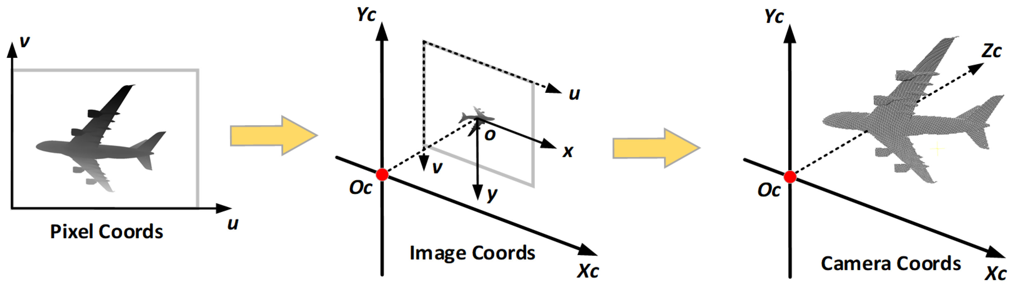
3. Methods
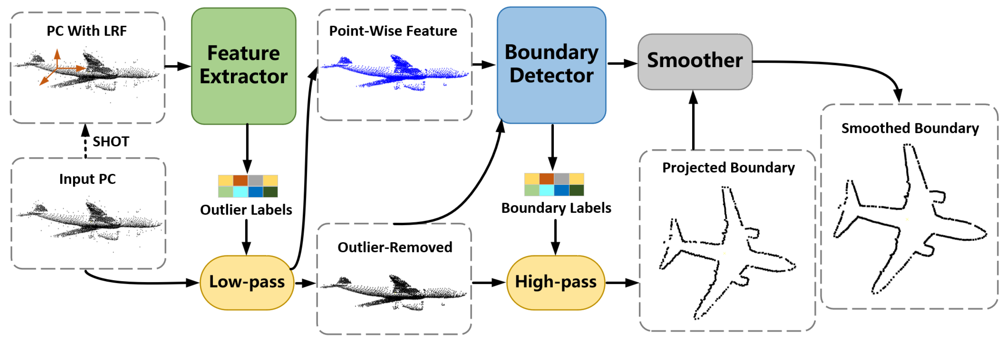
3.1. Overview
| Algorithm 1 Overall Pipeline of PcBD Processing Flow |
|
3.2. Feature-Extracting & Outlier Removal

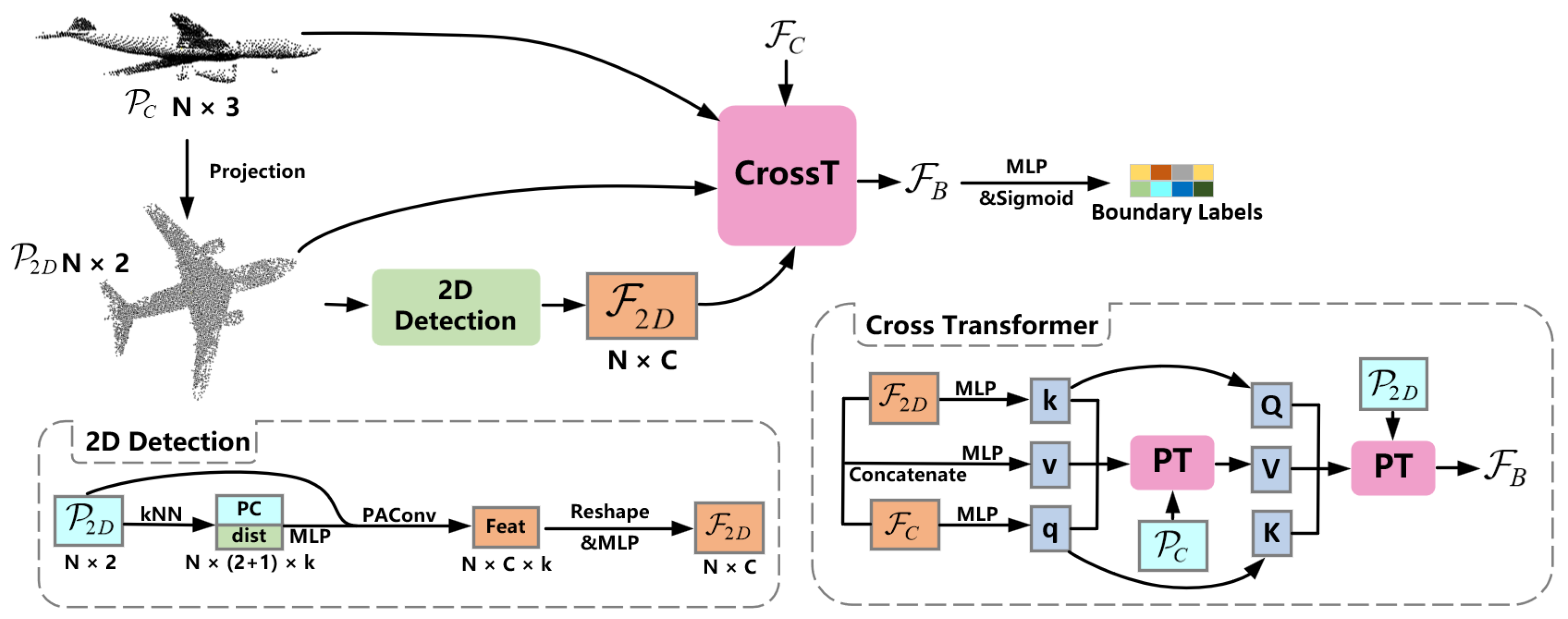
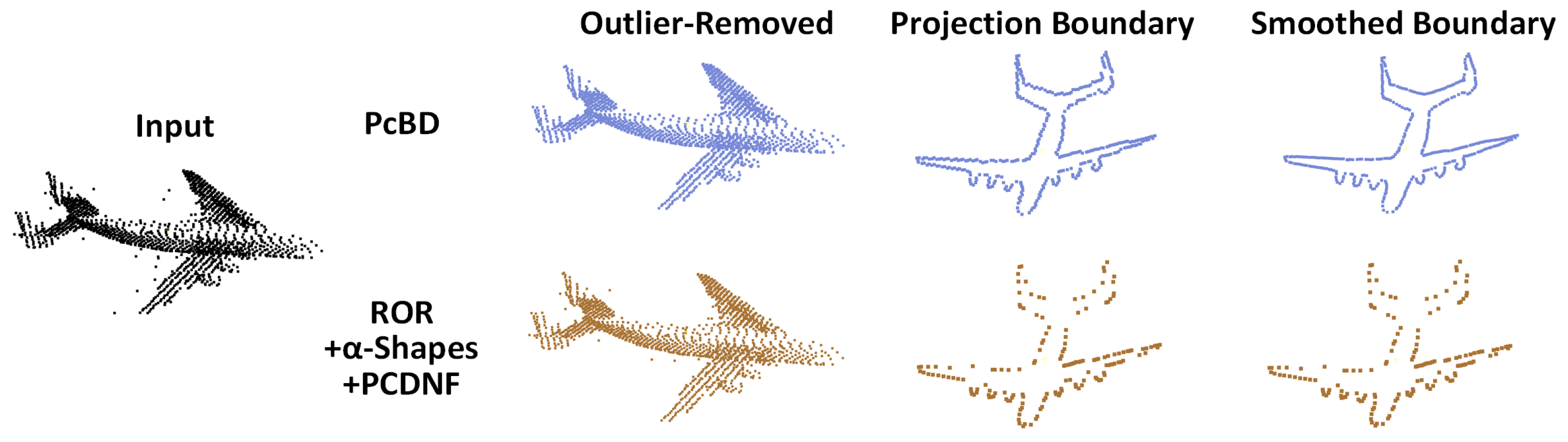
3.3. Boundary-Detecting
3.4. Smoothing
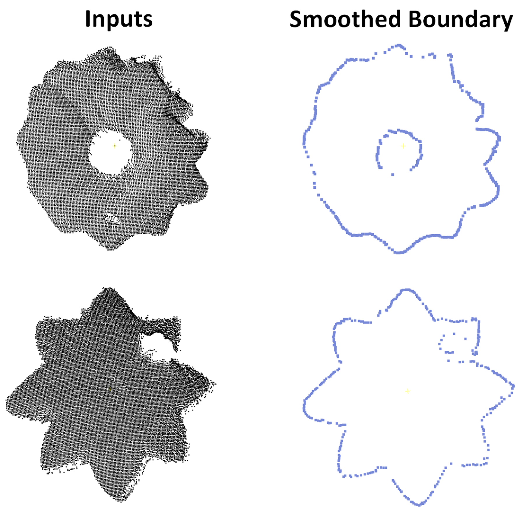
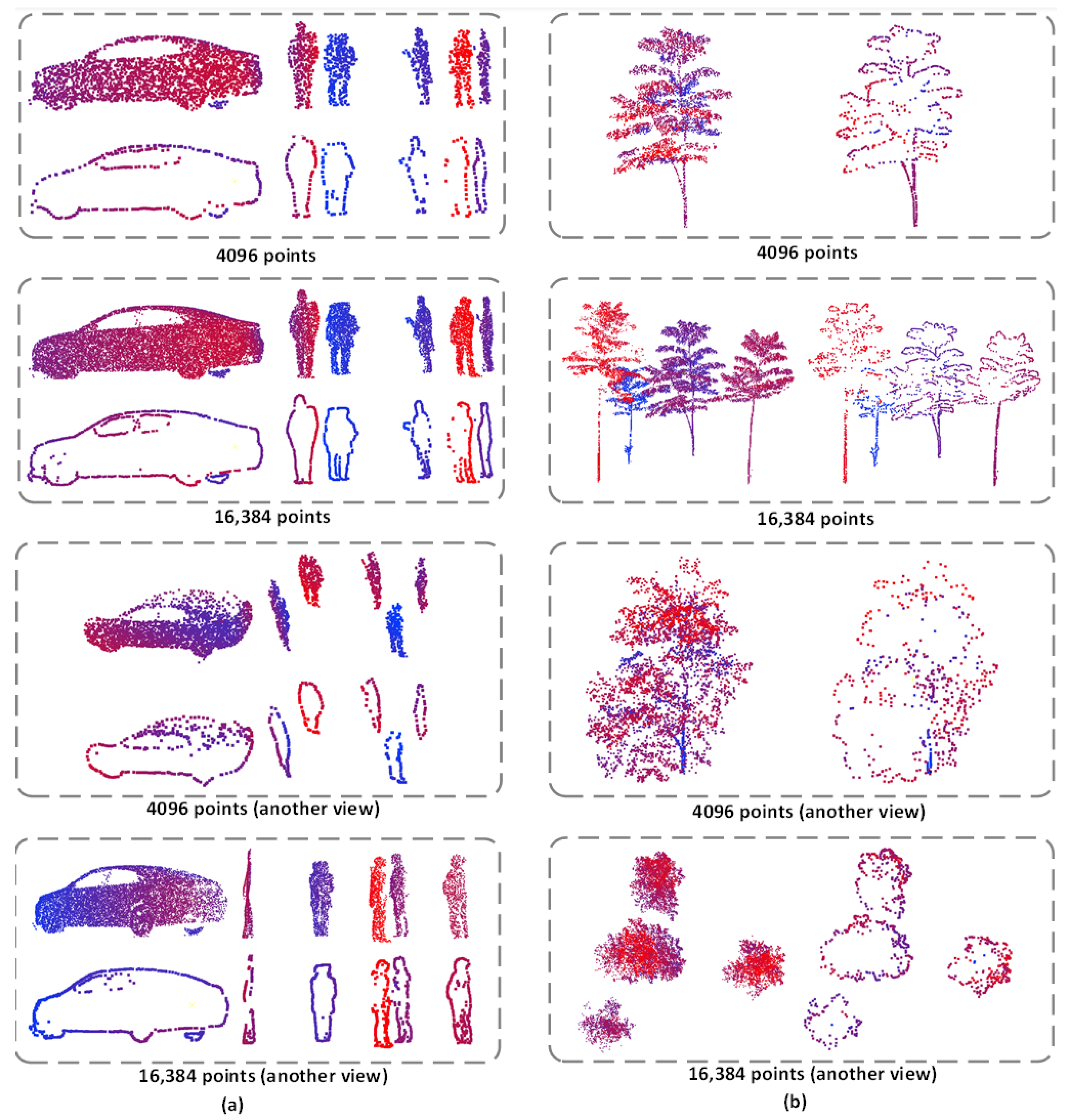
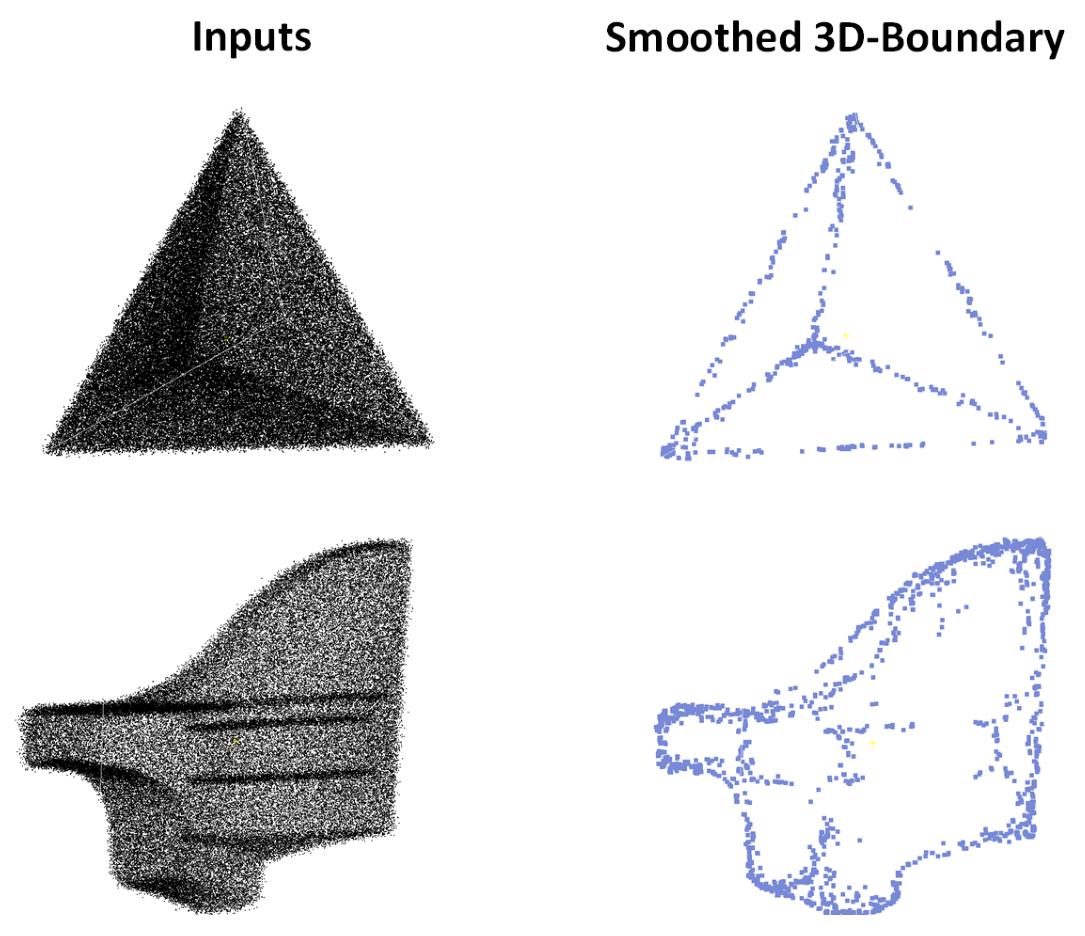
4. Experiments and Results
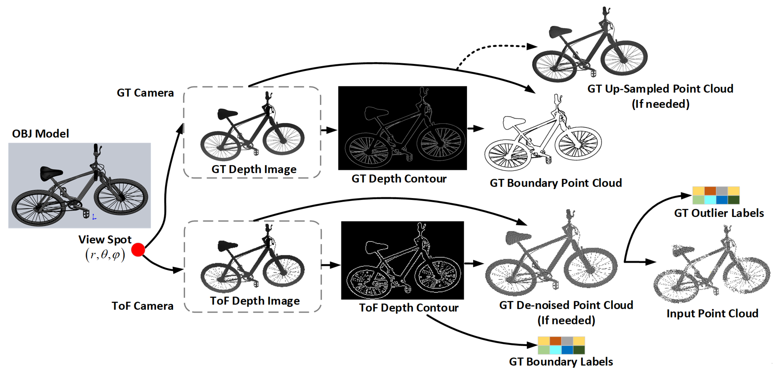
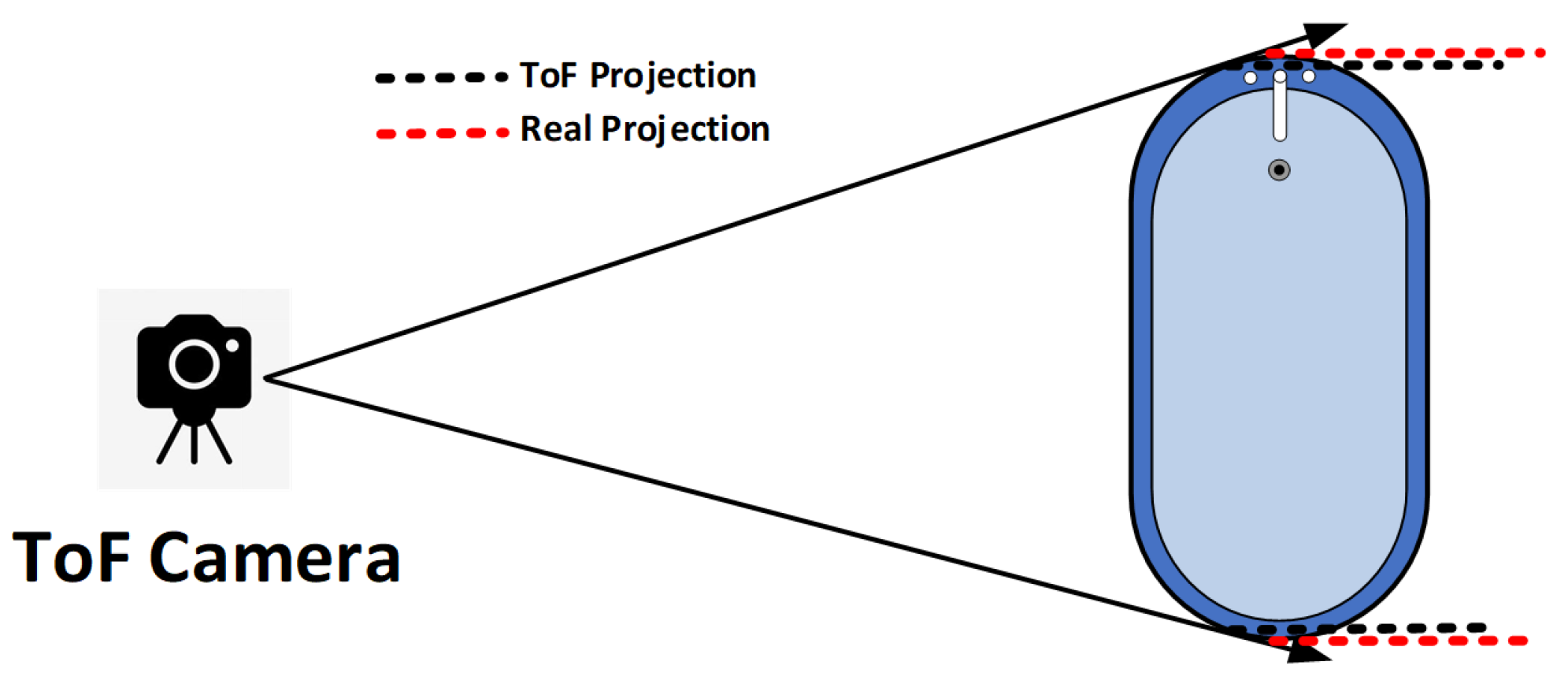
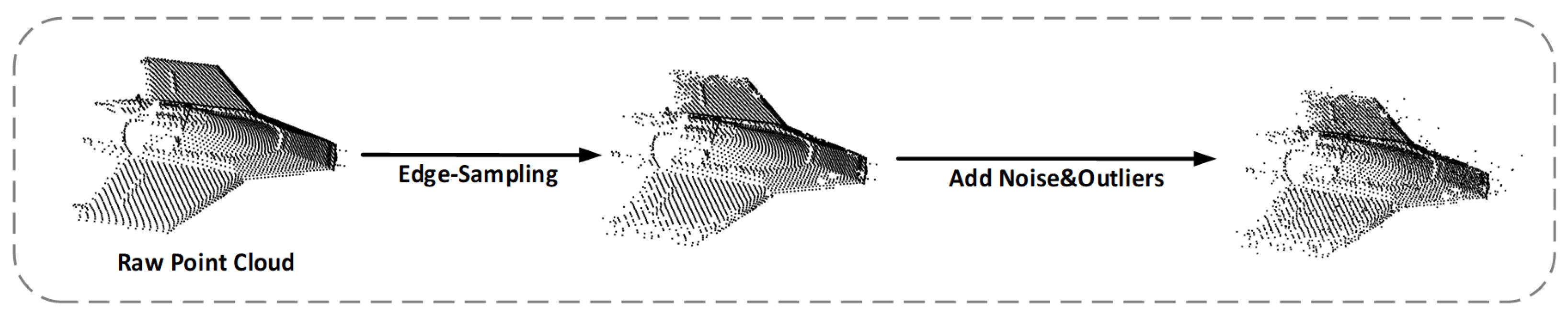
4.1. The Bound57 Dataset
4.2. Training
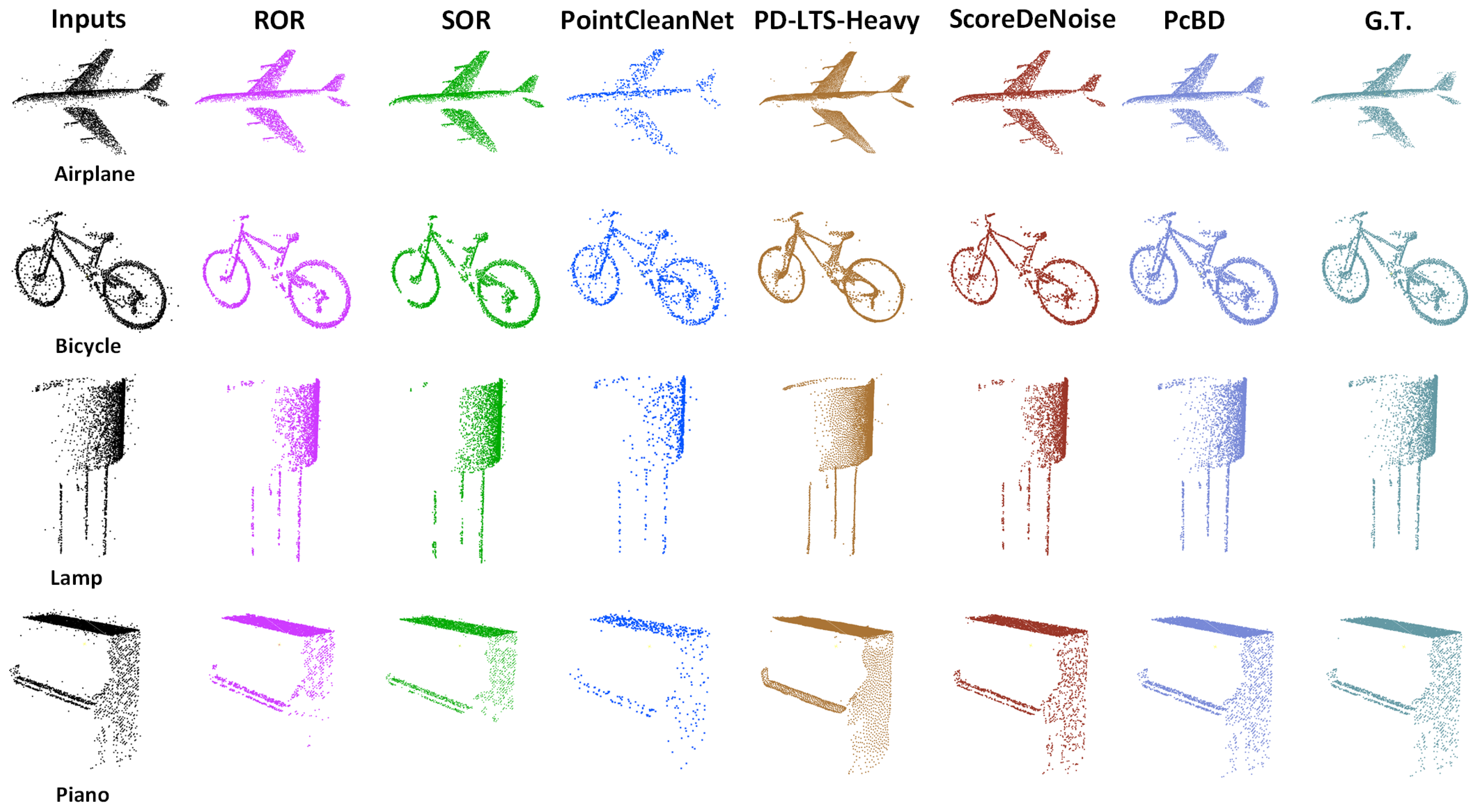
4.3. Results on Bound57
4.4. Other Experiments
4.5. Ablation Studies
5. Discussion
6. Conclusions
- A 89.47–99.30% reduction in Chamfer-L1 distance in outlier removal, outperforming methods such as ROR and PD-LTS;
- A 58.15–81.33% improvement in boundary detection accuracy over methods such as Grid-Contour and Adaptive -Shape methods;
- Superior smoothing results with an average Chamfer-L1 distance of 9.92, surpassing traditional methods such as MLS and modern networks such as Score de-noise.
- As a processing flow, significantly outperforms a processing flow consisting of three different advanced methods in completing the above tasks simultaneously.
Author Contributions
Funding
Institutional Review Board Statement
Informed Consent Statement
Data Availability Statement
Conflicts of Interest
Abbreviations
| ToF | Time of Flight |
| MLP | MultiLayer Perceptron |
| kNN | k-Nearest Neighbors |
| LRF | Local Reference Frame |
| GT | Ground Truth |
| CD | Chamfer Distance |
| BCE | Binary Cross Entropy |
References
- Henry, P.; Krainin, M.; Herbst, E.; Ren, X.; Fox, D. RGB-D Mapping: Using Kinect-Style Depth Cameras for Dense 3D Modeling of Indoor Environments. Int. J. Robot. Res. 2012, 31, 647–663. [Google Scholar] [CrossRef]
- Han, D. Research on Control System Design of Automobile Wind Tunnel Model Test. In Proceedings of the 2023 Asia-Europe Conference on Electronics, Data Processing and Informatics (ACEDPI), Prague, Czech Republic, 17–19 April 2023; pp. 15–19. [Google Scholar] [CrossRef]
- Inman, J.A.; Danehy, P.M. From Wind Tunnels to Flight Vehicles: Visualization and quantitative measurements supporting NASA’s space program. In Proceedings of the Optical Sensors and Sensing Congress, Washington, DC, USA, 22–26 June 2020; p. LW4E.1. [Google Scholar] [CrossRef]
- Tanner, C.L.; Clark, I.G.; Chen, A. Overview of the Mars 2020 parachute risk reduction activity. In Proceedings of the 2018 IEEE Aerospace Conference, Big Sky, MT, USA, 3–10 March 2018; pp. 1–11. [Google Scholar] [CrossRef]
- O’Farrell, C.; Muppidi, S.; Brock, J.M.; Van Norman, J.W.; Clark, I.G. Development of models for disk-gap-band parachutes deployed supersonically in the wake of a slender body. In Proceedings of the 2017 IEEE Aerospace Conference, Big Sky, MT, USA, 4–11 March 2017; pp. 1–16. [Google Scholar] [CrossRef]
- Salti, S.; Tombari, F.; Di Stefano, L. SHOT: Unique signatures of histograms for surface and texture description. Comput. Vis. Image Underst. 2014, 125, 251–264. [Google Scholar] [CrossRef]
- Zhao, H.; Jiang, L.; Jia, J.; Torr, P.; Koltun, V. Point Transformer. In Proceedings of the IEEE/CVF International Conference on Computer Vision, Montreal, BC, Canada, 11–17 October 2021. [Google Scholar]
- Wang, W.; You, X.; Chen, L.; Tian, J.; Tang, F.; Zhang, L. A Scalable and Accurate De-Snowing Algorithm for LiDAR Point Clouds in Winter. Remote Sens. 2022, 14, 1468. [Google Scholar] [CrossRef]
- Kurup, A.; Bos, J. DSOR: A Scalable Statistical Filter for Removing Falling Snow from LiDAR Point Clouds in Severe Winter Weather. arXiv 2021, arXiv:2109.07078. [Google Scholar]
- Digne, J.; Franchis, C. The Bilateral Filter for Point Clouds. Image Process. Line 2017, 7, 278–287. [Google Scholar] [CrossRef]
- Si, H.; Wei, Z.; Zhu, Z.; Chen, H.; Liang, D.; Wang, W.; Wei, M. LBF:Learnable Bilateral Filter For Point Cloud Denoising. arXiv 2022, arXiv:2210.15950. [Google Scholar]
- Huang, H.; Wu, S.; Gong, M.; Cohen-Or, D.; Ascher, U.M.; Zhang, H. Edge-aware point set resampling. ACM Trans. Graph. (TOG) 2013, 32, 1–12. [Google Scholar] [CrossRef]
- Zeng, J.; Cheung, G.; Ng, M.; Pang, J.; Yang, C. 3D Point Cloud Denoising using Graph Laplacian Regularization of a Low Dimensional Manifold Model. arXiv 2019, arXiv:1803.07252. [Google Scholar] [CrossRef]
- Hu, W.; Gao, X.; Cheung, G.; Guo, Z. Feature Graph Learning for 3D Point Cloud Denoising. IEEE Trans. Signal Process. 2020, 68, 2841–2856. [Google Scholar] [CrossRef]
- Qi, C.R.; Yi, L.; Su, H.; Guibas, L.J. PointNet++: Deep Hierarchical Feature Learning on Point Sets in a Metric Space. arXiv 2017, arXiv:1706.02413. [Google Scholar]
- Xu, M.; Ding, R.; Zhao, H.; Qi, X. PAConv: Position Adaptive Convolution with Dynamic Kernel Assembling on Point Clouds. arXiv 2021, arXiv:2103.14635. [Google Scholar]
- Ao, S.; Hu, Q.; Yang, B.; Markham, A.; Guo, Y. SpinNet: Learning a General Surface Descriptor for 3D Point Cloud Registration. arXiv 2021, arXiv:2011.12149. [Google Scholar]
- Thomas, H.; Qi, C.R.; Deschaud, J.E.; Marcotegui, B.; Goulette, F.; Guibas, L.J. KPConv: Flexible and Deformable Convolution for Point Clouds. arXiv 2019, arXiv:1904.08889. [Google Scholar]
- Seppänen, A.; Ojala, R.; Tammi, K. 4DenoiseNet: Adverse Weather Denoising from Adjacent Point Clouds. IEEE Robot. Autom. Lett. 2023, 8, 456–463. [Google Scholar] [CrossRef]
- Heinzler, R.; Piewak, F.; Schindler, P.; Stork, W. CNN-based Lidar Point Cloud De-Noising in Adverse Weather. IEEE Robot. Autom. Lett. 2020, 5, 2514–2521. [Google Scholar] [CrossRef]
- Zhao, X.; Wen, C.; Wang, Y.; Bai, H.; Dou, W. TripleMixer: A 3D Point Cloud Denoising Model for Adverse Weather. arXiv 2024, arXiv:2408.13802. [Google Scholar]
- Rakotosaona, M.; La Barbera, V.; Guerrero, P.; Mitra, N.J.; Ovsjanikov, M. PointCleanNet: Learning to Denoise and Remove Outliers from Dense Point Clouds. Comput. Graph. Forum 2020, 39, 185–203. [Google Scholar] [CrossRef]
- Duan, C.; Chen, S.; Kovacevic, J. 3D Point Cloud Denoising via Deep Neural Network based Local Surface Estimation. arXiv 2019, arXiv:1904.04427. [Google Scholar]
- Luo, S.; Hu, W. Differentiable Manifold Reconstruction for Point Cloud Denoising. In Proceedings of the 28th ACM International Conference on Multimedia, Seattle, WA, USA, 12–16 October 2020; pp. 1330–1338. [Google Scholar] [CrossRef]
- Hermosilla, P.; Ritschel, T.; Ropinski, T. Total Denoising: Unsupervised Learning of 3D Point Cloud Cleaning. arXiv 2019, arXiv:1904.07615. [Google Scholar]
- Luo, S.; Hu, W. Score-Based Point Cloud Denoising (Learning Gradient Fields for Point Cloud Denoising). In Proceedings of the 2021 IEEE/CVF International Conference on Computer Vision (ICCV), Montreal, QC, Canada, 17 October 2021; pp. 4563–4572. [Google Scholar] [CrossRef]
- Hyvarinen, A. Estimation of Non-Normalized Statistical Models by Score Matching. J. Mach. Learn. Res. 2005, 6, 695–709. [Google Scholar]
- Vogel, M.; Tateno, K.; Pollefeys, M.; Tombari, F.; Rakotosaona, M.J.; Engelmann, F. P2P-Bridge: Diffusion Bridges for 3D Point Cloud Denoising. In European Conference on Computer Vision; Springer: Cham, Switzerland, 2024. [Google Scholar]
- Li, Y.; Sheng, H. A single-stage point cloud cleaning network for outlier removal and denoising. Pattern Recognit. 2023, 138, 109366. [Google Scholar] [CrossRef]
- Li, X.; Lu, J.; Ding, H.; Sun, C.; Zhou, J.T.; Meng, C.Y. Risk-optimized Outlier Removal for Robust 3D Point Cloud Classification. arXiv 2024, arXiv:2307.10875. [Google Scholar] [CrossRef]
- Chand, D.R.; Kapur, S.S. An Algorithm for Convex Polytopes. J. ACM 1970, 17, 78–86. [Google Scholar] [CrossRef]
- Graham, R.L. An Efficient Algorithm for Determining the Convex Hull of a Finite Planar Set. Inf. Process. Lett. 1972, 1, 132–133. [Google Scholar] [CrossRef]
- Edelsbrunner, H.; Kirkpatrick, D.; Seidel, R. On the shape of a set of points in the plane. IEEE Trans. Inf. Theory 1983, 29, 551–559. [Google Scholar] [CrossRef]
- dos Santos, R.C.; Galo, M.; Carrilho, A.C. Extraction of Building Roof Boundaries From LiDAR Data Using an Adaptive Alpha-Shape Algorithm. IEEE Geosci. Remote Sens. Lett. 2019, 16, 1289–1293. [Google Scholar] [CrossRef]
- Peethambaran, J.; Muthuganapathy, R. A non-parametric approach to shape reconstruction from planar point sets through Delaunay filtering. Comput.-Aided Des. 2015, 62, 164–175. [Google Scholar] [CrossRef]
- Yang, Q.; Li, Z.; Liu, Z.; Jiang, X.; Gao, X. The Circle Pure Rolling Method for Point Cloud Boundary Extraction. Sensors 2025, 25, 45. [Google Scholar] [CrossRef]
- Bode, L.; Weinmann, M.; Klein, R. BoundED: Neural Boundary and Edge Detection in 3D Point Clouds via Local Neighborhood Statistics. arXiv 2022, arXiv:2210.13305. [Google Scholar] [CrossRef]
- Xiang, P.; Wen, X.; Liu, Y.S.; Cao, Y.P.; Wan, P.; Zheng, W.; Han, Z. SnowflakeNet: Point Cloud Completion by Snowflake Point Deconvolution with Skip-Transformer. arXiv 2021, arXiv:2108.04444. [Google Scholar]
- Paszke, A.; Gross, S.; Massa, F.; Lerer, A.; Bradbury, J.; Chanan, G.; Killeen, T.; Lin, Z.; Gimelshein, N.; Antiga, L.; et al. PyTorch: An Imperative Style, High-Performance Deep Learning Library. arXiv 2019, arXiv:1912.01703. [Google Scholar]
- Chang, A.X.; Funkhouser, T.; Guibas, L.; Hanrahan, P.; Huang, Q.; Li, Z.; Savarese, S.; Savva, M.; Song, S.; Su, H.; et al. ShapeNet: An Information-Rich 3D Model Repository. arXiv 2015, arXiv:1512.03012. [Google Scholar]
- Canny, J. A Computational Approach to Edge Detection. In Readings in Computer Vision; Fischler, M.A., Firschein, O., Eds.; Morgan Kaufmann: San Francisco, CA, USA, 1987; pp. 184–203. [Google Scholar] [CrossRef]
- Bradski, G. The OpenCV Library. Dr. Dobb’s J. Softw. Tools 2000, 25, 120–123. [Google Scholar]
- Yuan, W.; Khot, T.; Held, D.; Mertz, C.; Hebert, M. PCN: Point Completion Network. arXiv 2019, arXiv:1808.00671. [Google Scholar]
- Goodfellow, I.; Bengio, Y.; Courville, A. Deep Learning; MIT Press: Cambridge, MA, USA, 2016. [Google Scholar]
- Fan, H.; Su, H.; Guibas, L.J. A Point Set Generation Network for 3D Object Reconstruction from a Single Image. In Proceedings of the IEEE Conference on Computer Vision and Pattern Recognition (CVPR), Honolulu, HI, USA, 21–26 July 2017; pp. 605–613. [Google Scholar]
- Achlioptas, P.; Diamanti, O.; Mitliagkas, I.; Guibas, L. Learning Representations and Generative Models for 3D Point Clouds. In Proceedings of the International Conference on Machine Learning (ICML), Stockholm, Sweden, 10–15 July 2018; pp. 40–49. [Google Scholar]
- Rusu, R.B.; Cousins, S. 3D is here: Point Cloud Library (PCL). In Proceedings of the 2011 IEEE International Conference on Robotics and Automation, Shanghai, China, 9–13 May 2011; pp. 1–4. [Google Scholar] [CrossRef]
- Rusu, R.B. Semantic 3D Object Maps for Everyday Manipulation in Human Living Environments. KI-Künstliche Intelligenz 2010, 24, 345–348. [Google Scholar] [CrossRef]
- Anant, R.; Sunita, J.; Anand, J.; Kumar, M. A Density Based Algorithm for Discovering Density Varied Clusters in Large Spatial Databases. Int. J. Comput. Appl. 2010, 3, 1–4. [Google Scholar]
- Mao, A.; Yan, B.; Ma, Z.; He, Y. Denoising Point Clouds in Latent Space via Graph Convolution and Invertible Neural Network. In Proceedings of the 2024 IEEE/CVF Conference on Computer Vision and Pattern Recognition (CVPR), Seattle, WA, USA, 16–22 June 2024; pp. 5768–5777. [Google Scholar] [CrossRef]
- Gao, Y.; Chen, W.; Yu, C.; Yao, Y.; Xiao, T. Automatic extraction of building elevation contours based on LIDAR data. In Proceedings of the 2017 4th International Conference on Systems and Informatics (ICSAI), Hangzhou, China, 11–13 November 2017; pp. 1352–1357. [Google Scholar] [CrossRef]
- Sun, D.; Fan, Z.; Li, Y. Automatic extraction of boundary characteristic from scatter data. J. Huazhong Univ. 2008, 36, 82–84. [Google Scholar]
- Yu, L.; Li, X.; Fu, C.W.; Cohen-Or, D.; Heng, P.A. EC-Net: An Edge-aware Point set Consolidation Network. arXiv 2018, arXiv:1807.06010. [Google Scholar]
- Xie, Y.; Tu, Z.; Yang, T.; Zhang, Y.; Zhou, X. EdgeFormer: Local patch-based edge detection transformer on point clouds. Pattern Anal. Appl. 2025, 28, 11. [Google Scholar] [CrossRef]
- Loizou, M.; Averkiou, M.; Kalogerakis, E. Learning Part Boundaries from 3D Point Clouds. Comput. Graph. Forum 2020, 39, 183–195. [Google Scholar] [CrossRef]
- Han, X.F.; Jin, J.S.; Wang, M.J.; Jiang, W. Iterative guidance normal filter for point cloud. Multimed. Tools Appl. 2018, 77, 16887–16902. [Google Scholar] [CrossRef]
- Duan, C.; Chen, S.; Kovacevic, J. Weighted multi-projection: 3D point cloud denoising with tangent planes. In Proceedings of the 2018 IEEE Global Conference on Signal and Information Processing (GlobalSIP), Anaheim, CA, USA, 26–28 November 2018; pp. 725–729. [Google Scholar] [CrossRef]
- Leal, E.; Sanchez-Torres, G.; Branch, J.W. Sparse Regularization-Based Approach for Point Cloud Denoising and Sharp Features Enhancement. Sensors 2020, 20, 3206. [Google Scholar] [CrossRef] [PubMed]
- Alexa, M.; Behr, J.; Cohen-Or, D.; Fleishman, S.; Levin, D.; Silva, C. Computing and rendering point set surfaces. IEEE Trans. Vis. Comput. Graph. 2003, 9, 3–15. [Google Scholar] [CrossRef]
- Xu, Z.; Foi, A. Anisotropic Denoising of 3D Point Clouds by Aggregation of Multiple Surface-Adaptive Estimates. IEEE Trans. Vis. Comput. Graph. 2021, 27, 2851–2868. [Google Scholar] [CrossRef] [PubMed]
- Liu, Z.; Zhao, Y.; Zhan, S.; Liu, Y.; Chen, R.; He, Y. PCDNF: Revisiting Learning-Based Point Cloud Denoising via Joint Normal Filtering. IEEE Trans. Vis. Comput. Graph. 2024, 30, 5419–5436. [Google Scholar] [CrossRef]
- Zhang, D.; Lu, X.; Qin, H.; He, Y. Pointfilter: Point Cloud Filtering via Encoder-Decoder Modeling. arXiv 2020, arXiv:2002.05968. [Google Scholar] [CrossRef]
- Dong, Z.; Liang, F.; Yang, B.; Xu, Y.; Zang, Y.; Li, J.; Yuan, W.; Dai, W.; Fan, H.; Hyyppä, J.; et al. Registration of large-scale terrestrial laser scanner point clouds: A review and benchmark. ISPRS J. Photogramm. Remote Sens. 2020, 163, 327–342. [Google Scholar] [CrossRef]


| Methods/Results | Avg. | Airplane | Bench | Bicycle | Lamp | Microphone | Piano | Stove | Watercraft |
|---|---|---|---|---|---|---|---|---|---|
| DMRde-noise [24] | 14.43 | 13.83 | 13.77 | 14.29 | 16.48 | 17.46 | 14.10 | 15.26 | 12.49 |
| PointCleanNet [22] | 5.02 | 4.39 | 4.68 | 5.72 | 4.48 | 5.93 | 6.13 | 2.79 | 5.81 |
| Score de-noise [26] | 3.90 | 3.73 | 3.89 | 4.33 | 3.74 | 3.56 | 3.87 | 3.98 | 3.83 |
| PD-LTS-Heavy [50] | 3.79 | 3.17 | 3.92 | 4.39 | 3.13 | 3.22 | 3.85 | 4.08 | 3.62 |
| PD-LTS-Light [50] | 3.15 | 2.65 | 3.45 | 4.18 | 2.61 | 2.66 | 3.17 | 3.35 | 3.10 |
| DBSCAN [49] | 2.31 | 0.81 | 1.54 | 1.30 | 2.00 | 3.00 | 2.89 | 2.46 | 1.11 |
| SOR [48] | 1.38 | 0.58 | 0.96 | 0.98 | 1.10 | 1.07 | 1.70 | 1.77 | 0.73 |
| ROR [47] | 0.95 | 0.26 | 0.61 | 0.58 | 0.58 | 0.56 | 1.02 | 1.42 | 0.46 |
| PcBD (Ours) | 0.10 | 0.07 | 0.13 | 0.23 | 0.05 | 0.04 | 0.11 | 0.09 | 0.10 |
| Methods/Results | Avg. | Bag | Bowl | Car | Chair | Mug | Printer | Telephone |
|---|---|---|---|---|---|---|---|---|
| Normal-based [52] | 38.78 | 45.26 | 61.28 | 39.80 | 34.60 | 55.84 | 40.78 | 33.62 |
| Ada -Shapes [34] | 25.18 | 25.77 | 55.62 | 25.27 | 19.44 | 47.28 | 46.39 | 19.07 |
| -Shapes [33] | 23.02 | 27.11 | 48.50 | 19.79 | 16.62 | 29.50 | 50.12 | 27.62 |
| Grid-Contour [51] | 17.30 | 13.36 | 32.65 | 16.40 | 14.89 | 31.14 | 29.20 | 20.21 |
| PcBD (Ours) | 7.24 | 10.55 | 14.20 | 7.08 | 7.72 | 9.54 | 6.42 | 3.23 |
| Methods/Results | Avg. | Bathtub | Camera | Earphone | Flowerpot | Motorbike | Pillow | Rifle | Train |
|---|---|---|---|---|---|---|---|---|---|
| DMRde-noise [24] | 61.99 | 81.24 | 55.51 | 54.01 | 81.91 | 33.96 | 63.26 | 25.12 | 37.30 |
| PointCleanNet [22] | 59.90 | 66.98 | 57.65 | 43.59 | 73.29 | 31.21 | 75.18 | 23.54 | 46.42 |
| PD-LTS-Heavy [50] | 16.03 | 18.86 | 15.90 | 13.21 | 17.75 | 11.86 | 22.59 | 8.21 | 12.53 |
| Score de-noise [26] | 14.85 | 17.39 | 14.10 | 11.75 | 17.35 | 10.67 | 19.18 | 6.89 | 11.45 |
| PD-LTS-Light [50] | 13.33 | 15.56 | 12.89 | 12.32 | 15.56 | 10.53 | 15.94 | 7.13 | 10.55 |
| Bilateral Filter [10] | 12.03 | 14.48 | 11.46 | 9.42 | 13.95 | 8.99 | 14.90 | 5.76 | 8.60 |
| AdaMLS [60] | 11.01 | 11.43 | 9.97 | 7.70 | 14.11 | 7.71 | 10.87 | 5.23 | 8.39 |
| SparseReg [58] | 11.85 | 13.59 | 11.31 | 10.36 | 12.76 | 9.67 | 12.09 | 8.27 | 9.97 |
| Iter-norm-filter [56] | 10.97 | 13.06 | 10.30 | 9.50 | 13.05 | 8.24 | 12.27 | 5.63 | 8.04 |
| PointFilter [62] * | 10.86 | 12.78 | 10.33 | 8.96 | 12.24 | 8.73 | 12.41 | 6.85 | 8.19 |
| W-Multi-Proj [57] | 10.29 | 12.86 | 9.04 | 10.00 | 12.32 | 8.36 | 12.90 | 5.57 | 7.72 |
| MLS [59] | 10.21 | 12.51 | 9.86 | 8.62 | 12.34 | 8.68 | 11.33 | 5.41 | 7.98 |
| PCDNF [61] * | 9.28 | 11.08 | 8.55 | 7.59 | 10.87 | 7.43 | 10.69 | 5.08 | 6.71 |
| PcBD (Ours) | 9.92 | 8.29 | 7.04 | 19.60 | 13.24 | 8.75 | 9.68 | 4.37 | 8.05 |
| Version | Outlier | Boundary | Smoothing |
|---|---|---|---|
| Removing | Detecting | ||
| PcBD | 0.100 | 7.239 | 9.918 |
| PCA Normal Calculation | 0.109 | 7.533 | 10.201 |
| Regular Conv in Set-Abstraction | 0.116 | 8.078 | 10.638 |
| Regular PT in FE | 0.111 | 8.031 | 10.545 |
| Only 2D Projection in BD | 0.107 | 8.338 | 10.782 |
| No Cross Attention (2D and 3D) | 0.105 | 7.705 | 9.999 |
| Smoothing Only Using 3D Boundary | 0.100 | 7.241 | 10.504 |
Disclaimer/Publisher’s Note: The statements, opinions and data contained in all publications are solely those of the individual author(s) and contributor(s) and not of MDPI and/or the editor(s). MDPI and/or the editor(s) disclaim responsibility for any injury to people or property resulting from any ideas, methods, instructions or products referred to in the content. |
© 2025 by the authors. Licensee MDPI, Basel, Switzerland. This article is an open access article distributed under the terms and conditions of the Creative Commons Attribution (CC BY) license (https://creativecommons.org/licenses/by/4.0/).
Share and Cite
Sun, S.; Huang, J.; Zhao, S.; Huang, T. PcBD: A Novel Point Cloud Processing Flow for Boundary Detecting and De-Noising. Appl. Sci. 2025, 15, 7073. https://doi.org/10.3390/app15137073
Sun S, Huang J, Zhao S, Huang T. PcBD: A Novel Point Cloud Processing Flow for Boundary Detecting and De-Noising. Applied Sciences. 2025; 15(13):7073. https://doi.org/10.3390/app15137073
Chicago/Turabian StyleSun, Shuyu, Jianqiang Huang, Shuai Zhao, and Tengchao Huang. 2025. "PcBD: A Novel Point Cloud Processing Flow for Boundary Detecting and De-Noising" Applied Sciences 15, no. 13: 7073. https://doi.org/10.3390/app15137073
APA StyleSun, S., Huang, J., Zhao, S., & Huang, T. (2025). PcBD: A Novel Point Cloud Processing Flow for Boundary Detecting and De-Noising. Applied Sciences, 15(13), 7073. https://doi.org/10.3390/app15137073