An Optimal 3D Visualization Method for Integral Imaging Optical Display Systems Using Depth Rescaling and Field-of-View Resizing

Abstract

Integral imaging is a promising 3D sensing and visualization technique that enables full-parallax and continuous viewpoint reconstruction. However, challenges, such as depth distortion and a limited field-of-view (FoV), can compromise the quality of 3D visualization. This paper proposes a method to optimize the display of captured 3D scenes for integral imaging optical display systems. To achieve high-quality 3D visualization, the captured 2D images are processed to align the depth range and field-of-view with the specification of the display system. The proposed approach computationally scales the captured scene nonuniformly across three dimensions, integrating a depth scaling process and a scene resizing process. By generating synthetic 2D elemental images tailored to a specific 3D display system, the proposed method can enhance depth accuracy and display adaptability. Experimental results demonstrate that our method significantly improves 3D display quality, offering a more immersive and visually accurate representation.

1. Introduction

Integral imaging (InIm) was first proposed by G. Lippmann in 1908 [1,2]. As one of the autostereoscopic systems [1,2,3,4,5,6], InIm can produce a 3D optical image with continuous viewing points and does not need special glasses, which makes it a favored technique for 3D optical visualization. InIm has been applied in various imaging applications, such as 3D display [7,8,9,10], depth estimation [11,12], task specific 3D sensing, detection and recognition, etc. [13,14]. Conventional integral imaging includes two general steps: pickup of 3D objects information, and 3D reconstruction. In the pickup process, a lenslet array and an imaging sensor are used to capture light rays from the objects in 3D space. Passing through each lenslet, object information is recorded by the image sensor as a 2D image. Each captured 2D image is referred to as an elemental image (EI), and contains the intensity and directional information of light rays from the objects. For 3D reconstruction, a display device is used to visualize the elemental images. Light from the display screen passes through the identical lenslet array used in the pickup process, retraces the same optical route, and then converges at the original point of the 3D objects.

One problem for InIm 3D optical display is the pseudoscopic nature of the 3D imaging. The convex and concave portions of 3D objects are reversed for viewers. Some approaches have been investigated to solve such a problem. A concave–convex convention method was proposed in [15] by rotating each elemental image by 180 degrees around its center. Additionally, a general algorithm for pseudoscopic to orthoscopic imaging convention, known as the Smart Pseudoscopic-to-Orthoscopic Conversion (SPOC) method, was introduced in [16]. This method also provides full control over display parameters to generate synthetic elemental images for an InIm optical display system.

Another challenge in InIm optical display is the limitation of image depth. A simple method to improve image depth was proposed in [17] by displaying a 3D image within the real and virtual imaging fields. The multiple-plane pseudoscopic to orthoscopic conversion (MP POC) method [18] offers more precise pixel mapping, leading to improve 3D display results. By utilizing these methods, enhanced 3D visualization in InIm optical display becomes possible.

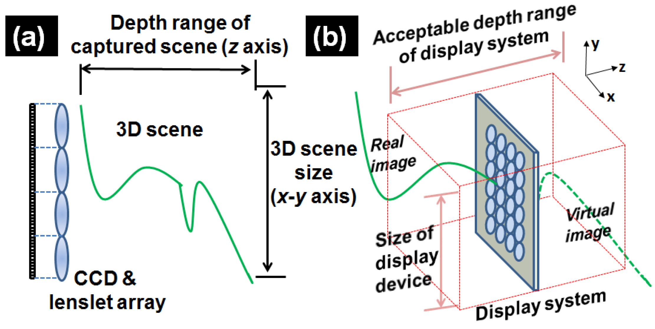
For a given display system, the acceptable display range (along the z-axis) is constrained by light diffraction and the resolution of the pixelated imaging device. Additionally, the field-of-view (FoV) of a display device (x-y axis plane) is fixed. However, in practical applications, the captured 3D scene often has varying depth ranges and scene sizes, which may not match with the constraints of the display system. As shown in Figure 1, when the depth range of a 3D scene exceeds the capabilities of the system or the scene size surpasses dimensions of the display device, achieving a fully visible and high-quality 3D display becomes challenging. To address this issue, some research works have been reported. In [19], a scaling method that adjusts the special ray sampling rate using a moving array-lenslet technique (MALT) was investigated. Multi-depth fitting fusion was investigated in [20]. Another method in [21] employed an intermediate-view reconstruction technique to magnify 3D images in an InIm system. In [22,23,24], tunable focus techniques have been introduced, utilizing cropped elemental image and focus-tunable lens. Recently, transmissive mirror and semi-transparent mirror have been integrated with an integral imaging display for depth of field and resolution-enhanced 3D display [25]. However, these methods primarily focused on two-dimensional scaling (depth in z or field of view in x-y) and may require pre-processing or specialized devices.

Table 1. Comparison between methods for optimized integral imaging optical display.

Method	Enhancement		Other Limitation
	Depth	Field of View
SPOC [16]
Use of real and virtual fields [17]	X		Low resolution, mainly for static 3D image
MP SPOC [18]	X
MALT [20]		X
IVRT-based scaling [21]	X	X	Uniformly scaling, needs identical lens array
Tunable focus techniques [22,23,24]	X		Need specialized devices
Transmissive mirror and semi-transparent mirror [25]	X	X	Need specialized devices
Proposed method in this paper	X	X

presents a comparative summary of the methods described above, including key features and corresponding limitations of each approach.

To optimally display the captured 3D scene for a specific display system, we propose a computational approach that regenerates elemental images through depth rescaling and scene resizing. The depth rescaling process adjusts the depth range of the captured scene to match the acceptable range of the display device, while the scene resizing process modifies the field-of-view to fit the display dimensions. By fully utilizing the display capacities of the system (acceptable depth range in z direction and the field-of-view in x-y directions), optimal display results for a specific display system can be achieved.

This paper is organized as follows: Section 2 details the proposed depth rescaling (z-axis). In Section 3, the proposed scene resizing (x-y axis) process is explained. Section 4 details the 3D display experimental results. Conclusions are given in Section 5.

2. Depth Rescaling Process (Z Axis)

To rescale the depth of a captured scene and match the depth capacity of a 3D display system, we processed a depth rescaling method. This implementation works by generating a synthetic elemental image array. The depth range of the scene can then be adjusted in the newly generated elemental image array by setting multiple virtual pinhole arrays in the synthetics capture process.

Similar to the MP POC method [16,18], the generation of synthetic elemental images includes two stages:

• Simulated Display:
  • The captured elemental images (from the real pickup process) are first virtually displayed on multiple reference planes (RPs). The parameters in the simulated display process include (i) the pitch of the lenslet array (p), (ii) the gap (g) between the captured elemental images and the lenslet array, and (iii) the focal length (f) of the lenslet array; they should be identical to the parameters of the real pickup process.
• Synthetic Capture:
  • A virtual pinhole array (VPA) is set up to implement pixel mapping from the reference planes to an image sensor, then regenerate the synthetic elemental image array (EIA). The virtual pinhole array parameters depend on the specific 3D display system (display device and lenslet array).

The complete procedure is illustrated in Figure 2. Note that to optimize the use of the display system’s depth range, the display plane needs to be positioned at the center of the reconstructed 3D scene [18]. Additionally, the synthetic elemental image array is loaded onto the display device for 3D InIm display. The position of the virtual pinhole array needs be identical to the position of the lenslet array placed in front of the display device. In addition, the MP POC method not only performs depth rescaling but also mitigates the issue of inaccurate depth information [18]. By employing multiple reference planes (see Figure 2), the MP-POC method enables accurate pixel mapping for objects located at different depths.

In conventional synthetic capture, a single virtual pinhole array is positioned at a specific location. As a result, the depth information recorded by the synthetic elemental images remains unchanged from the original depth range of the scene. To adapt the captured 3D scene to the depth range of a display system, we propose to use multiple virtual pinhole arrays at different positions in the synthetic capture stage.

Each virtual pinhole array corresponds to a specific reference plane and records information about it. The multiple elemental image arrays captured through this process are then superimposed to create a new elemental image array. The distance between each reference plane and its corresponding virtual pinhole array in the synthetic capture process is set to match the distance between the image and the display device in the 3D display process. By carefully configuring these parameters (distance between each reference plane and its corresponding virtual pinhole array, d, as shown in Figure 2), the depth of the 3D scene can be effectively rescaled.

The proposed depth rescaling method includes the following steps:

• Depth Analysis: Obtain the depth information of the 3D scene in each captured elemental image and separate the 3D scene into multiple depth regions.
• Reference Plane Calculation: Determine the number of reference planes. For each reference plane, obtain its position.
• Virtual Pinhole Array Distance Calculation: Calculate the distance (d) between each reference plane and its corresponding virtual pinhole array.
• Pixel Mapping: Map pixels from the real captured elemental images to the corresponding reference plane (simulated display).
• Synthetic Capture: Generate new elemental images from each reference plane to their corresponding virtual pinhole array.
• Superimposition: Combine the elemental image arrays to create a synthetic captured elemental image array with rescaled depth.

In the proposed method, we adopt the depth estimation method in [11] to statistically estimate the depth information of the 3D scene. The depth estimation uses the statistics of spectral radiation in an object space to infer the depth of the surfaces in the 3D scene, and this method aligns well with the architecture of integral imaging optical sensing, sharing the same specifications and structural framework as the proposed process, which ensures procedural consistency. The number of the reference planes and the position of each reference plane can be calculated by segmenting the depth range of the original 3D scene into several sub-regions in the z direction. The boundary between two adjacent regions can be regarded as the position of the reference plane.

For further explanation, we denote the number of the reference planes as N_RP, and we set the N_RP reference planes to cover the depth range of the 3D scene. Note that the N_RP reference planes separate the depth range into N_RP − 1 sub-regions. The index of the reference planes ranges from 1 to N_RP, and the first reference plane is set at the position where the surface of the object is closest to the lenslet array. The distance between the lenslet array and the ith reference plane in the simulated display stage can be expressed as follows:

$$z_{RP}^i=z_{rear}+{\displaystyle \frac{d_o}{N_{RP}-1}}\times (i-1)$$

(1)

where z_rear is the closest distance between the surface of the object and the lenslet array. d_o is the depth range of the 3D scene and N_RP is the number of reference planes.

For optimal display, we set the rescaled depth of the 3D image to the depth range of the display system in order to fully utilize the capacities of the 3D display. To display both the real and virtual scene in the display system, the virtual pinhole array needs to be set at the center of the 3D scene in the synthetic capture stage [23]. The distance of d_i between the ith reference plane and the corresponding ith virtual pinhole array in the synthetic capture process is equal to the distance between the ith reference plane and the display plane in the 3D display process:

$$d^i={\displaystyle \frac{d_s}{N_{RP}-1}}\times [{\displaystyle \frac{N_{RP}}{2}}-(i-{\displaystyle \frac{1}{2}})]$$

(2)

where d_s is the depth range of the display system. From Equations (1) and (2), the distance between the ith virtual pinhole array and the lenslet array can be calculated as follows:

$$z_p^i=z_{RP}^i+d^i$$

(3)

In the simulated display stage, the distance between two neighboring reference planes is $\mathrm{\Delta }RP=d_o/(N_{RP}-1)$, after the synthetic capture stage, a new elemental image array is generated by superimposing the synthetic captured elemental images. The distance between two reference planes recorded in the regenerated elemental image array is $\mathrm{\Delta }d=d_s/(N_{RP}-1)$. The range of the reference planes corresponds to the depth range of the 3D scene. Therefore, the depth range of the 3D scene is rescaled by a factor of M_d:

$$M_d={\displaystyle \frac{d_s}{d_o}}$$

(4)

With the proposed depth rescaling method discussed in Section 2, the 3D image can be optimized to match the display systems with a specific depth range. In this manner, the display quality of the 3D scene can be improved substantially.

3. Scene Resizing Process (X-Y Axis)

The conventional InIm display remains the original size of the 3D scene. As the dimension of the display device is fixed, it may be difficult to display a large 3D scene which is over the display capacity. In this section, we propose a scene resizing method to adjust the field-of-view. This method is implemented computationally in the simulated display stage by proportionally resetting (i) the pitch (p) of the pinhole array, and (ii) the gap between the captured elemental images and the pinhole. The resized field-of-view will match to the specific size of the display device.

Figure 3 shows the principle of the scene resizing method in the computationally simulated display process, where a reference plane is set at z_RP from the lenslet array for simulated display. Figure 3a shows the simulated display with the original pickup parameters. The pixel size on the reference plane is denoted by s₁. By computationally rescaling the pixel size on the reference plane with a factor of variable M_s, the 3D scene size can be adjusted. The position of the rescaled reference plane still locates at z_RP, and the rescaled pixel size on the reference plane denoted as s₂ is shown in Figure 3b; the expressions for s₁ and s₂ are as follows:

$$\left\{\begin{array}{c}{s}_1={\displaystyle \frac{S_{CCD}}{EI\_resol}}\times {\displaystyle \frac{z_{RP}}{g_1}}\\ s_2={\displaystyle \frac{S_{CCD}}{EI\_resol}}\times {\displaystyle \frac{z_{RP}}{g_2}}\end{array}\right.$$

(5)

where S_CCD is the sensor size, EI_resol is the resolution of each captured elemental image, g₁ is the gap between the sensor and the lenslet array for simulated display with the original pickup parameters. g₂ is the gap between the sensor and the pinhole array for simulated display with the scene resizing method.

We focus on the same pixels (the green and red pixels shown in Figure 3) in the original reference plane and the new reference plane. Both the green pixel and the red pixel are on the principal optical axis of the corresponding two neighboring lenslets (pinholes). The two principal optical axes are shown in red and green dashed lines, respectively, in Figure 3. The lateral distance between the two pixels is equal to the pitch of the lenslet array (p₁). In order to resize the scene, we update the pitch of the virtual pinhole in the simulated display stage. To avoid nonlinear distortions in this process, the two specific pixels mentioned above should be located on the principal optical axes of the corresponding pinholes. The new distance between these resized pixels is equal to the pitch of the pinhole array (p₂). The pitch of the two pixels can be calculated as follows:

$$\left\{\begin{array}{c}{p}_1=n\times s_1\\ p_2=n\times s_2\end{array}\right.$$

(6)

where n is the pixel number between the two pixels. Using similar triangle geometry, the resized pixel size on the new reference plane can be expressed as follows:

$$s_2=s_1\times M_s={\displaystyle \frac{S_{CCD}}{EI\_resol}}\times {\displaystyle \frac{z_{RP}}{g_1}}\times M_s$$

(7)

By combining Equations (5)–(7), the relationship between the gaps in the real pickup stage (g₁) and the field-of-view resizing simulated display stage (g₂) can be calculated. In addition, we are able to obtain the relationship between the original pitch of lenslet array (p₁) in the real pickup process and the pitch of the pinhole array (p₂) in the scene resizing method by the following expression:

$$\left\{\begin{array}{c}{g}_2=g_1/M_s\\ p_2=p_1\times M_s\end{array}\right.$$

(8)

Based on Equation (8), by properly setting the gap (g) between the captured elemental images and the pinhole array, and the pitch (p) of the pinhole array in the simulated display stage, the field-of-view resizing process can be realized.

With the proposed scene resizing processing discussion in this section, the field of view of the 3D image can be optimized to match the display systems for the optimized 3D optical display.

4. 3D Integral Imaging Display Experimental Results

To demonstrate the feasibility of the proposed method, two groups of InIm optical display experiments are conducted. The first group is for a computer-generated 3D scene in 3dsMax. The second group is for a real 3D scene. Elemental images were captured by the synthetic aperture integral imaging technology [26].

Figure 4 shows two examples of the captured elemental images and the corresponding depth maps of the computer-generated 3D scene. A pyramid and a box are located at 190 mm and 490 mm in front of the camera. The depth range of the 3D scene is over 300 mm, exceeding the depth range of the display system (80 mm~100 mm). For the depth map, the pixel intensity represents the depth of the points recorded by the camera. As shown in Figure 4b, the further the objects are located, the lower the intensities will appear on the depth map. Parameters of the computer-generated 3D scene and the computational InIm pickup process are shown in

Table 2. Specifications of computer-generated integral imaging pickup.

Description	Parameters
Total number of elemental images (EIs)	11 (H) × 11 (V)
Resolution on each EI	2000 (H) × 2000 (V)
Sensor pitch	15 mm (H) × 15 mm (V)
Focal length	18.1 mm
Field-of-view of each sensor	50 degree
Angular resolution	0.025 degree
Distances between the surface of objects and the pickup plane	Pyramid: 190 mm Box: 490 mm
3D scene depth range	300 mm
Scene size	Approx. 220 mm (H) × 120 mm (V)

.

For the computer-generated 3D scene, the nearest surface (z_rear) is located at 190 mm from the camera. We reset the depth range (d_s) as 80 mm. Based on Equations (1)–(3), two reference planes are selected to cover the 3D scene at 190 mm and 490 mm. The virtual pinhole arrays are calculated at 230 mm and 450 mm. The pixel information on the two reference planes is synthetically captured by their corresponding virtual pinhole arrays with distances (d) of −40 mm and 40 mm, respectively. By superimposing the synthetic elemental images, a synthetic elemental image array is generated with a rescaled depth range of 80 mm centering at the display plane. The scene size is about 220 mm (Horizontal, H) × 120 mm (Vertical, V). Consider the field-of-view of the virtual pinhole array, the area for synthetic capture is approximately 140 mm (H) × 69 mm (V) at ±40 mm from the pinhole array. The 3D scene can be fully recorded by the synthetically generated elemental image array with a resize factor of 0.5.

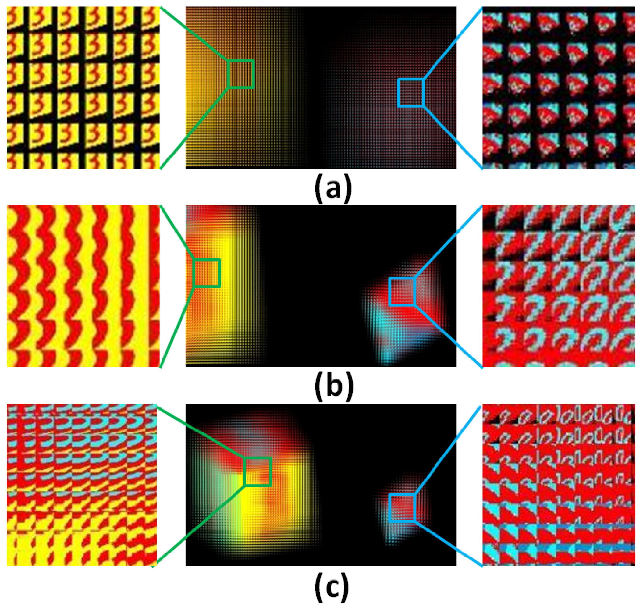
Figure 5 shows the generated synthetic elemental image arrays for 3D display. The elemental image array generated by the SPOC method remains the original depth and size information of the 3D scene, as shown in Figure 5a. Figure 5b is the elemental image array with the depth rescaling process. The depth range has been rescaled from 300 mm to 80 mm. By combining the depth rescaling and the scene resizing, a synthetic captured elemental image array is newly generated, as shown in Figure 5c. The depth of the 3D scene has been rescaled from 300 mm to 80 mm on the z axis, and the scene has been resized on the x-y axis by a factor of 0.5. The enlarged elemental images show that by setting multiple reference planes, pixel information of a large depth 3D scene can be mapped correctly, so that detailed information can be captured with the depth rescaling process. However, due to the limited resolution of the display device, only partial information of the 3D scene can be captured by the elemental image array. With the scene resizing process, the 3D scene is fully recorded by the synthetic captured elemental image array. Note that due to the use of multiple reference planes that better match the object’s depth during the depth rescaling process (as discussed in Section 2), details in the pyramid are well preserved in the elemental images, as shown in Figure 5c. In contrast, with the conventional SPOC method, which uses a single reference plane, details in the pyramid are lost, as illustrated in Figure 5a, because the reference plane is far from the actual object depth.

Another group of experiments for a real 3D scene obtained by the synthetic aperture integral imaging technique was conducted. The 3D scene consists of a white bear toy and a globe with a large depth range of 425 mm. Both objects are over 2000 mm away from the pickup camera array; the parameters of the 3D scene and the synthetic aperture pickup process are shown in

Table 3. Specifications of synthetic aperture integral imaging pickup—real 3D scene.

Description	Parameters
Total number of elemental images (EIs)	5 (H) × 8 (V)
Resolution on each EI	2808 (H) × 1872 (V)
Sensor pitch	36 mm (H) × 24 mm (V)
Focal length	35 mm
Field-of-view of each sensor	14 (H) × 9.4 (V) degree
Angular resolution	0.005 degree
Distances between the surface of objects and the pickup plane	Globe: 1975 mm Bear toy: 2400 mm
3D scene depth range	425 mm
Object sizes	Approx. 330 mm (H) × 220 mm (V)

.

Two of the captured elemental images and the corresponding estimated depth maps are shown in Figure 6. In the estimated depth maps, the pixel color represents the relative position of the corresponding 3D points recorded by the camera. In the depth map, pixel intensities encode the depth information of the points captured by the camera. Objects that are farther away appear with higher intensity values.

For the real 3D scene group, the nearest surface (z_rear) is located at 1975 mm in front of the pickup camera. We rescale the depth range (d_s) to 100 mm. Based on Equations (1)–(3), two reference planes were selected to encompass the 3D scene at 1975 mm and 2400 mm. The corresponding virtual pinhole arrays are calculated at 2025 mm and 2350 mm. Two reference planes are synthetically captured by their respective virtual pinhole array, positioned at −50 mm and 50 mm relative to the plane. By superimposing the synthetic elemental images, the synthetic elemental image array is regenerated with a rescaled depth range of 100 mm, centered at the display plane. The scene size is about 330 mm (H) × 200 mm (V). Considering the field-of-view of the virtual pinhole array within the depth range, the synthetic capture area is approximately 117 mm (H) × 72 mm (V) at ±50 mm from the pinhole array. The 3D scene is fully recorded by the regenerated elemental image array with a resizing factor of 0.35.

Figure 7 illustrates the synthetically captured elemental image arrays for the 3D display. The generated elemental image array by the conventional SPOC method preserves the original depth and size information of the 3D scene, as shown in Figure 7a. In contrast, Figure 7b presents the elemental image array after applying the depth rescaling process, where the depth range of the real 3D scene has been rescaled from 425 mm to 100 mm. By integrating both depth rescaling and scene resizing, the resulting elemental image array is depicted in Figure 7c. In this case, the depth range of the 3D scene is scaled from 425 mm to 100 mm along the z axis, while the scene size is adjusted on the x-y axis with a resizing factor of 0.35. Note that due to the use of multiple reference planes that better match the object’s depth during the depth rescaling process (as discussed in Section 2), details in globe are well preserved in the elemental images, as shown in Figure 7c. In contrast, with the conventional SPOC method, which uses a single reference plane, details in the globe are lost, as illustrated in Figure 7a, because the reference plane is far from the actual object depth.

In the experiment, a smart phone monitor and a lenslet array were used for the InIm 3D display system, as shown in Figure 8 The gap (g) between the display device and the lenslet array is equal to the focal length (f) of each optical lenslet. The display device is set in the center of the reconstruction space; therefore, the real image floating outside of the display plane and the virtual image converging inside of the display plane will be visualized synchronously for 3D display. Due to light diffraction and pixelated imaging device, the depth range of this display system is around 80mm to 100mm, centering at the display plane. Parameters of the display system for the experiment are listed in

Table 4. Specifications of integral imaging 3D display.

Description	Parameters
Display device	Smart phone monitor
Size of display panel	102 mm (H) × 57 mm (V)
Resolution of display device	1920 (H) × 1080 (V)
Pixel size of display device	Approx. 53 μm
Total number of elemental images (EIs)	96 (H) × 54 (V)
Pixel number on each EI	20 (H) × 20 (V)
Pitch of lenslet array	1 mm
Focal length of a lenslet	3.3 mm
Field-of-view	17.23 degree

.

The 3D display results of the computationally generated 3D scene are shown in Figure 9. Figure 9a presents three display results for the computer-generated 3D scene. From left to right, the images represent (i) the display result with the original object parameters, where depth range remains 300 mm without scene resizing; (ii) the display result after rescaling the depth from 300 mm to 80 mm along the z-axis, without scene resizing; and (iii) the display result after combing depth rescaling (form 300 mm to 80 mm along the z-axis) with field-of-view resizing on the x-y axis using a factor of 0.5. Figure 9b displays the five different viewpoint results from various perspectives of the computer-generated 3D scene.

The 3D display results of the real 3D scene are shown in Figure 10. Figure 10a presents the three display results for the real large-depth 3D scene. From left to right, the images represent (i) the display result with the original object parameters, where the depth range remains 425 mm; (ii) the display result after rescaling the depth from 425mm to 100 mm along the z-axis, without scene resizing; and (iii) the display result after combining depth rescaling (from 425 mm to 100 mm along the z axis) with scene resizing on the x-y axis using a factor of 0.35. Figure 10b shows the five different viewpoints results for the real 3D scene.

By applying the depth rescaling process, the 3D images can be displayed within the depth range of the display system. Due to the use of multiple reference planes that better align with the object’s depth during the depth rescaling process (as discussed in Section 2), the 3D display demonstrates improved viewing quality. Specifically, in the computer-generated integral imaging group, the box and pyramid maintain clearer details in the reconstructed 3D image, as shown in Figure 9a(iii). In contrast, with the conventional SPOC method, which uses a single reference plane, both the box and the pyramid appear with lower viewing quality—surface features, such as numbers and letters, are lost, as shown in Figure 9a(i). For the real 3D scene group, the clarity and structural details of the bear toy and the globe are well preserved in the 3D display when using the MP-POC method, as shown in Figure 10a(iii). Conversely, under the SPOC method, both the bear toy and the globe appear blurred, with poorly defined edges and shapes, as shown in Figure 10a(i). Additionally, the scene resizing process (as discussed in Section 3) ensures that the field-of-view of the 3D image matches the display device, allowing the entire 3D scene to be displayed without cropping. The display results show improved quality while maintaining the relative positions of objects in the 3D image without distortion.

In this section, we have presented experimental results of a 3D optical display using both a computer-generated (CG) 3D scene and a real-world captured 3D scene. The results confirm the feasibility of the proposed methods discussed in Section 2 and Section 3.

5. Conclusions

In this paper, we propose a practical technique to optimize the display of a captured 3D scene in an integral imaging optical display system by nonuniformly rescaling the depth range along the z-axis and resizing the field-of-view of a captured scene along the x-y axes. Using this approach, synthetically captured elemental images can be computationally regenerated to match the depth range and field-of-view of a specific 3D display system. Additionally, this technique allows focusing on specific parts of the 3D scene to enhance detail visibility. By fully utilizing the capabilities of the display system, both real and computer-generated 3D display experiments have demonstrated the feasibility of the proposed method in generating elemental images that align with the depth range and size requirements of a specified display system for optimal 3D visualization. The proposed method may face limitations when the scaling factor significantly exceeds one, as detailed information of the 3D scene must be computationally synthesized for accurate elemental image generation and 3D optical display. Further research will explore integrating machine learning algorithms to enhance the generation of synthetic elemental images, depth estimation, reduce noise and distortion, as well as extract details from original elemental images for high-resolution 3D optical displays.