Optimizing Car Collision Detection Using Large Dashcam-Based Datasets: A Comparative Study of Pre-Trained Models and Hyperparameter Configurations

Abstract

The automatic identification of traffic collisions is an emerging topic in modern traffic surveillance systems. The increasing number of surveillance cameras at urban intersections connected to traffic surveillance systems has created new opportunities for leveraging computer vision techniques for automatic collision detection. This study investigates the effectiveness of transfer learning utilizing pre-trained deep learning models for collision detection through dashcam images. We evaluated several state-of-the-art (SOTA) image classification models and fine-tuned them using different hyperparameter combinations to test their performance on the car collision detection problem. Our methodology systematically investigates the influence of optimizers, loss functions, schedulers, and learning rates on model generalization. A comprehensive analysis is conducted using 7 performance metrics to assess classification performance. Experiments on a large dashcam-based images dataset show that ResNet50, optimized with AdamW, a learning rate of 0.0001, CosineAnnealingLR scheduler, and Focal Loss, emerged as the top performer, achieving an accuracy of 0.9782, F1-score of 0.9617, and IoU of 0.9262, indicating a strong ability to reduce false negatives.

1. Introduction

Road traffic accidents represent one of the most critical public health issues of the modern era, exacting a devastating toll on human life and global economies. According to the World Health Organization (WHO), approximately 1.19 million lives are lost annually due to road collisions, with an additional 50 million individuals sustaining severe injuries [1]. These road accidents also impact the GDP of countries, as countries allocate nearly 3% of their annual GDP to address medical expenses, infrastructure repairs, and productivity losses linked to traffic incidents. These numbers rise even more in developing countries, where traffic safety rules are sometimes lenient and emergency response systems are inadequate, which fuels poverty and public health inequality in developing countries [2]. Moreover, according to the National Safety Council (NSC) [3], in 2023, car collisions claimed 19,400 lives out of the 44,762 total motor vehicle deaths in the United States, making up over 43% of the fatalities.

The inherent unpredictability of road accidents poses a difficult challenge to efforts to mitigate them. Collisions frequently arise from dynamic, non-linear interactions among human error, environmental conditions, and mechanical failures—factors that defy straightforward modeling [4,5]. Traditional reactive approaches, such as post-accident crash analysis or manual surveillance, suffer from critical limitations: they are labor-intensive, prone to human error, and incapable of enabling real-time intervention [6]. For instance, delayed accident detection on highways or in construction zones increases secondary risks, including prolonged congestion and delayed emergency response, which collectively increase economic losses and public frustration. The advancement in computer vision and deep learning offers transformative potential to address these gaps. Automated systems capable of real-time collision detection could revolutionize road safety by enabling proactive measures, from rerouting traffic to dispatching first-aid teams within seconds of an incident [7].

Recent research has leveraged deep learning for traffic-related applications, including vehicle detection [8,9,10], pedestrian tracking [11], and accident severity assessment [12,13,14]. Zhou [15] proposed an attention-based Stack ResNet for Citywide Traffic Accident Prediction framework which combines static spatial data with dynamic spatio-temporal information using a ResNet-based model and an attention mechanism to prioritize temporally relevant features and incorporates a speed inference module to address missing speed data. Jaspin et al. [16] proposed an automated, real-time Accident Detection and Severity Classification System that leverages YOLOv5 to identify accidents in video images and a machine learning classifier to categorize them into mild, moderate, or severe levels, triggering rapid alerts to authorities. To reduce latency and network usage in emergency detection, Banerjee et al. [17] proposed a Deep Learning-Based Car Accident Detection Framework which employs a 2D CNN on edge nodes for local video processing while offloading essential data to the cloud for further analysis.

Huang et al. [18] proposed the challenge of detecting near-accidents at traffic intersections in real-time, such as sudden lane changes or pedestrian crossings. They introduce a two-stream (spatial and temporal) convolutional network architecture designed for real-time detection, tracking, and near-accident prediction. The spatial stream uses the YOLO algorithm to detect vehicles and potential accident regions in individual video frames, while the temporal stream analyzes motion features across multiple frames to generate vehicle trajectories. By combining these spatial and temporal features, the system computes collision probabilities, flagging high-risk regions when trajectories intersect or come too close. Le et al. [19] proposed a two-stream deep learning network called Attention R-CNN to tackle the inability of traditional object detection methods to recognize not just the presence of objects but also their characteristic properties, such as whether they are safe, dangerous, or crashed, present in autonomous driving systems. The first stream leverages a modified Faster R-CNN to detect object bounding boxes and their classes, while the second stream, employs an attention mechanism to integrate global scene context with local object features, enabling the recognition of properties like “crashed” or “dangerous”. Javed et al. [20] address the shortcomings of existing accident detection systems, such as high false-positive rates, vehicle-specific compatibility issues, and high implementation costs, which delay emergency responses and increase road fatalities in smart cities. They developed a low-cost IoT kit equipped with sensors to collect real-time data like speed, gravitational force, and sound, which is transmitted to the cloud. A deep learning model based on YOLOv4, fine-tuned with ensemble transfer learning and dynamic weights, processes this data alongside video footage from a Pi camera to verify accidents and minimize false detections. Amrouche et al. [21] proposed a convolutional neural network (CNN)-based model for car crash detection using dashcam images, aiming to enable rapid and precise accident identification. Praveen et al. [22] proposed a framework that integrates IoT sensors with machine learning to enable real-time accident detection and risk prediction. IoT sensors installed on vehicles continuously collect data such as speed, acceleration, brake force, and lane deviation, transmitting this information wirelessly to a central system. The data are then processed using the Adaptive Random Forest algorithm that dynamically learns from incoming data to identify patterns indicative of accidents or high-risk situations. When parameters exceed predefined thresholds, such as excessive speed or sudden braking, the system issues alerts to drivers and may activate safety mechanisms like automatic braking. Pre-trained models have shown promising results in transfer learning scenarios, adapting to specialized tasks with limited data [23,24]. However, their application to car collision detection using dashcam images remains underexplored, particularly in optimizing hyperparameter configurations for real-world deployment.

This study provides a systematic evaluation of SOTA deep learning architectures for car collision detection to test their adaptability and performance under different hyper parameter settings. We fine-tune seven pre-trained models (

Table 1. Pre-trained models used for car collision detection.

Model	Number of Parameters	Weights Used
ResNet50	25,557,032	IMAGENET1K_V2
ResNet101	44,549,160	IMAGENET1K_V1
EffcientNet-B2	9,109,994	IMAGENET1K_V1
DenseNet121	7,978,856	IMAGENET1K_V1
MobileNetV3 (L)	5,483,032	IMAGENET1K_V2
ConvNeXt (B)	88,591,464	IMAGENET1K_V1
ViT-B-16	86,567,656	IMAGENET1K_V1

) under varied hyperparameter configurations (

Table 2. Parameters tested for car collision detection models.

Parameter	Value 1	Value 2	Value 3	Value 4
Scheduler	Step-LR	ReduceLROnPlateau	CosineAnnealingLR	CosineAnnealing WarmRestarts
Loss Function	Label Smoothing	Focal Loss	Cross Entropy	-
Optimizer	SGD	Adam	AdamW	-
Learning Rate	0.01	0.001	0.0001	-

) to identify optimal trade-offs between accuracy, computational efficiency, and localization reliability. The proposed framework holds significant practical implications. By automating collision detection, municipalities can reduce reliance on error-prone manual monitoring, accelerate emergency response times, and dynamically optimize traffic signals to mitigate congestion.

The rest of this paper is organized as follows: The Section 2 outlines the processes of data collection, data labeling, model selection, model customization, loss functions, optimizers, schedulers, and the training pipeline. The Section 3 explains the benchmark metrics for each model, and the Section 4 presents comparative findings of all the best models selected for each performance metric. The Section 5 explores the effects of different parameters in detail, while the Conclusion provides a summary and final remarks.

2. Methodology

The proposed framework for automatic car collision detection leverages transfer learning on pre-trained deep learning models with fine-tuning on a road car collision dataset. The pre-trained models were taken from the torchvision v0.22.1 library with ImageNet1K weights. The details of the model used, their number of parameters, and weights are provided in Table 1. Figure 1 shows the flow of our proposed car collision detection system.

2.1. Data Collection, Labeling, and Preparation

This section describes the data collection, labeling, and data preparation procedures. In Section 2.1.1, the process of car collision dataset collection from dashcam videos and their labeling process is explained. Section 2.1.2 describes the preprocessing and augmentation techniques applied to standardize and enhance the dataset for model training.

2.1.1. Data Collection and Labeling

We have created a comprehensive dataset from dashcam videos taken from YouTube, containing both collision events and normal driving scenarios. We collected a diverse set of more than 120 dashcam videos involving car collisions with a duration between 5 s and 8 s. Each video was further processed to extract the frames containing collision or no collision. Each extracted frame was labeled manually. All extracted frames were initially labeled by a single annotator to maintain consistency across the dataset, and the final labels were subsequently verified by another annotator to ensure accuracy and reliability. During the labeling process, the frames exhibiting visible collision cues and frames closer to the collision were labeled as ‘collision’, while those without such events were labeled as ‘no-collision’. After the labeling, the dataset was partitioned using stratified sampling with an 80/20 split (training and test sets), and the training set was further split into training and validation subsets (80/20 split). Figure 2 shows the train and test data distribution in our experiments. Due to the inherent imbalance between collision and non-collision frames, the training data were balanced using the RandomOverSampler from the imblearn library. This step ensured that minority collision classes were adequately represented, thereby reducing bias during model learning [25]. While RandomOverSampler was selected to balance the collision and non-collision classes due to its simplicity and effectiveness, we also considered the Synthetic Minority Oversampling Technique (SMOTE) and class-weighted loss functions. However, RandomOverSampler was chosen as it preserved original data integrity, whereas SMOTE’s synthetic samples risked introducing noise in the dashcam dataset, and class-weighted losses required extensive tuning.

2.1.2. Data Preprocessing and Augmentation

After the data labeling, data preprocessing was applied to standardize inputs and improve model robustness. Images were resized to 224 × 224 pixels and normalized using ImageNet mean and standard deviation (mean = [0.485, 0.456, 0.406], std = [0.229, 0.224, 0.225]) to standardize pixel value distributions. Horizontal Flip (p = 0.5) and Vertical Flip (p = 0.3) were applied to imitate varied perspectives. We have also applied Random Brightness and Contrast Adjustments (p = 0.2) to accommodate for variations in illumination.

2.2. Model Selection and Customization

In our experiments, we systematically evaluated seven pre-trained models as defined in Table 1 to identify the most effective model for car collision detection. All models were initialized with pre-trained weights from the ImageNet dataset, allowing them to start from a solid foundation of general image understanding. This transfer learning approach not only speeds up the training process but also improves performance on the task of collision detection by leveraging knowledge gained from a much larger and more diverse dataset.

During the fine-tuning process, we modified the last classification layers of each network to match pre-trained deep learning models for recognizing collisions in a binary classification setting. We customized each model to predict only two results: “collision” or “no-collision”, instead of maintaining the default output layers normally meant for multi-class problems. To streamline this process across different architectures, we built a unified framework that automatically finds and replaces the final classification layers. We replaced the last fully connected layer for models using a classification based on fully connected layers, and for transformer-based models, we updated the classification head accordingly. In every case, we introduced a new linear layer that outputs binary values (collision’, ‘no-collision’). These outputs are then passed through a SoftMax activation function to convert them into probabilities, making the predictions easy to interpret. This approach allows us to take full advantage of the powerful features already learned by these models on large datasets while fine-tuning them for the specific task of collision detection.

2.3. Loss Functions, Optimizers, and Schedulers

This section covers the choices of loss functions, optimizers, and learning rate schedulers used in training the models. Section 2.3.1 describes the three loss functions employed to address class imbalance and improve generalization. Section 2.3.2 details the optimizers selected for effective gradient handling and learning rate adjustment. Section 2.3.3 outlines the learning rate schedulers that dynamically adjust the learning rate to optimize training.

2.3.1. Loss Functions

We used three different loss functions to tackle the challenges of class imbalance and encourage more reliable learning. These loss functions bring unique strengths to the training process.

• Binary Cross Entropy (BCE) Loss: BCE loss is a standard choice for classification tasks, and it measures the difference between the predicted probabilities and the actual labels. It effectively penalizes incorrect predictions as it takes the full probability distribution into account.
• Focal Loss: Focal Loss is very useful when the dataset is highly imbalanced. Traditional loss functions tend to be influenced too much by examples that are easy to classify, which can cause the model to overlook the minority class. Focal Loss addresses this problem by reducing the importance of those easy examples and putting more focus on harder, misclassified examples, which makes it particularly useful for improving performance on underrepresented classes [26,27].
• Label Smoothing Loss: This loss was used to tackle the issue of overconfident predictions, which often harm generalization, especially in noisy or imbalanced data [28]. Instead of treating labels as absolute, this method softens them slightly. By applying a smoothing factor of 0.1, the model spreads a small portion of the label’s certainty across other classes. This encourages the model to be less certain in its predictions, helping to reduce overfitting and improve its ability to generalize.

2.3.2. Optimizers

In this study, the optimization process was carefully tailored using specific combinations of optimizers and learning rate schedulers to make sure that each model learned efficiently and adapted well throughout training.

Optimizers were chosen based on how they handle gradients and adjust learning over time.

• SGD (Stochastic Gradient Descent), enhanced with momentum (set to 0.9) and weight decay, offered a steady and reliable learning path. By accumulating gradients across iterations, it helped the model converge smoothly.
• Adam brought adaptive learning by adjusting learning rates based on both the average and variance of past gradients, which is especially helpful for handling sparse or noisy updates.
• AdamW, a refined version of Adam, separated weight decay from the update step, leading to better regularization and often improved generalization.

2.3.3. Schedulers

Learning rate schedulers were added to fine-tune the optimization process further. The schedulers used in our experiments are given below:

• StepLR gradually decreased the learning rate at set intervals, nudging the model toward convergence as training progressed.
• ReduceLROnPlateau watched the validation loss closely and reduced the learning rate only when improvements stalled—helpful for escaping local minima.
• CosineAnnealingLR and CosineAnnealingWarmRestarts [29] follow a cosine-shaped curve to gently reduce the learning rate and occasionally reset it, encouraging the model to explore new possibilities during training.

All optimizer and scheduler settings, including learning rates, momentum, and weight decay, were carefully tuned through experimentation. This setting ensured the models could not only learn robust features effectively but also stay robust against class imbalance and other training challenges.

2.4. Training Pipeline

We trained each model for 20 epochs on an NVIDIA GPU RTX 4080 with a batch size of 24. To prevent overfitting and save training time, early stopping was also implemented. StepLR reduced the learning rate by a factor of 0.1 every 10 epochs, while ReduceLROnPlateau kept monitoring the validation loss and adjusted only when improvements plateaued.

The experimental design involves a comprehensive set of hyperparameter configurations for training seven deep learning models. Each configuration is defined by a unique combination of four key components: the loss function, learning rate, optimizer, and scheduler. There are three loss functions, three learning rates, three optimizers, and four schedulers used in our experiments. The total number of distinct configurations is calculated by multiplying the number of options for each component: 3 (loss functions) × 3 (learning rates) × 3 (optimizers) × 4 (schedulers) = 108 configurations for one model. Figure 3 illustrates this combinatorial structure through a tree diagram, where each path from the root to a leaf node represents one such configuration. For clarity, the diagram partially expands the tree, showing the full branching for one loss function and partial branching for others, with the understanding that this pattern extends to all options. Each of these 108 configurations is then applied to each of the seven models, resulting in a total of 108 × 7 = 756 training runs. This systematic approach ensures a thorough exploration of the hyperparameter space, enabling a robust analysis of how different settings influence model performance across various metrics.

3. Evaluation Metrics

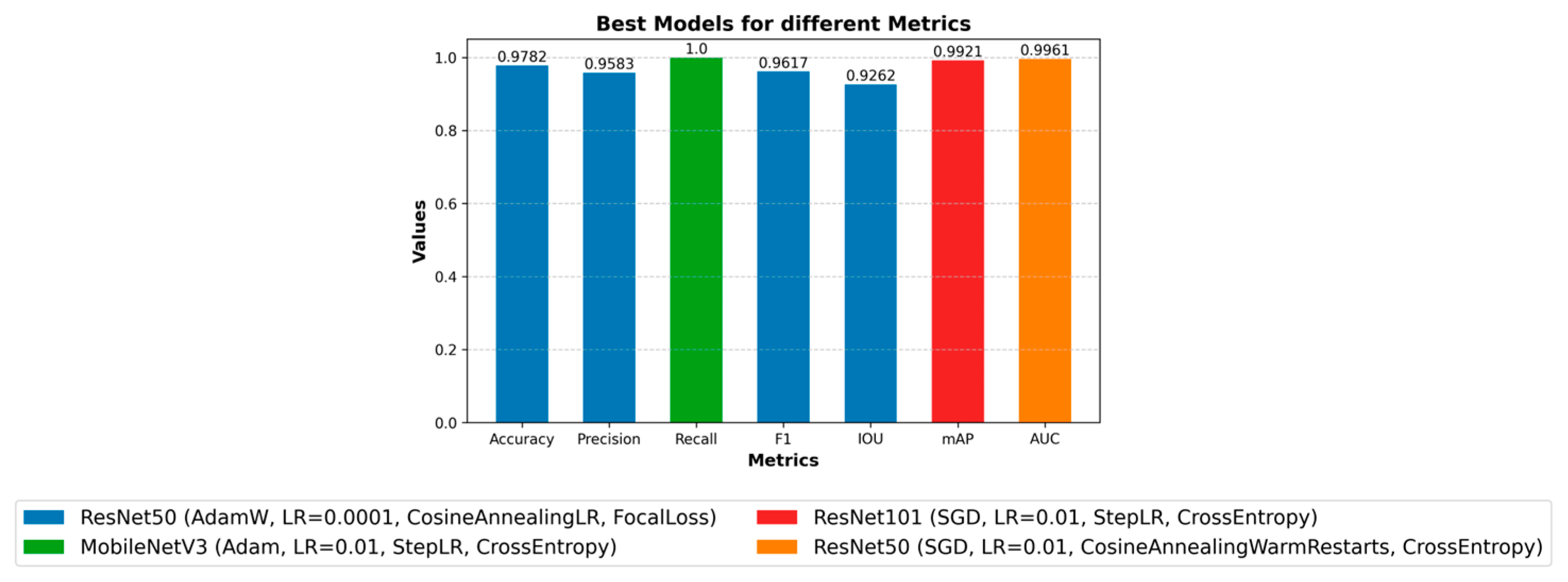
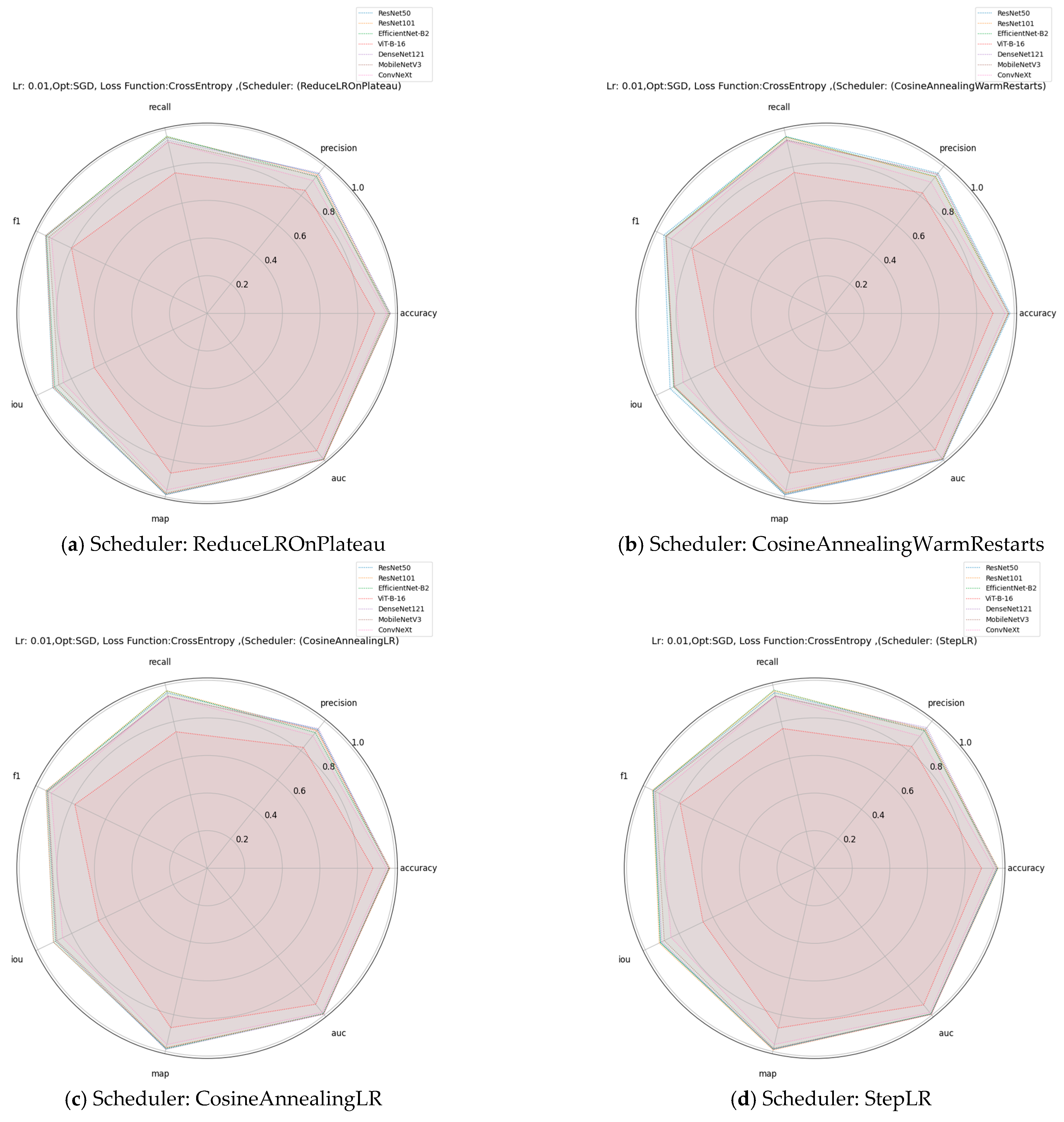
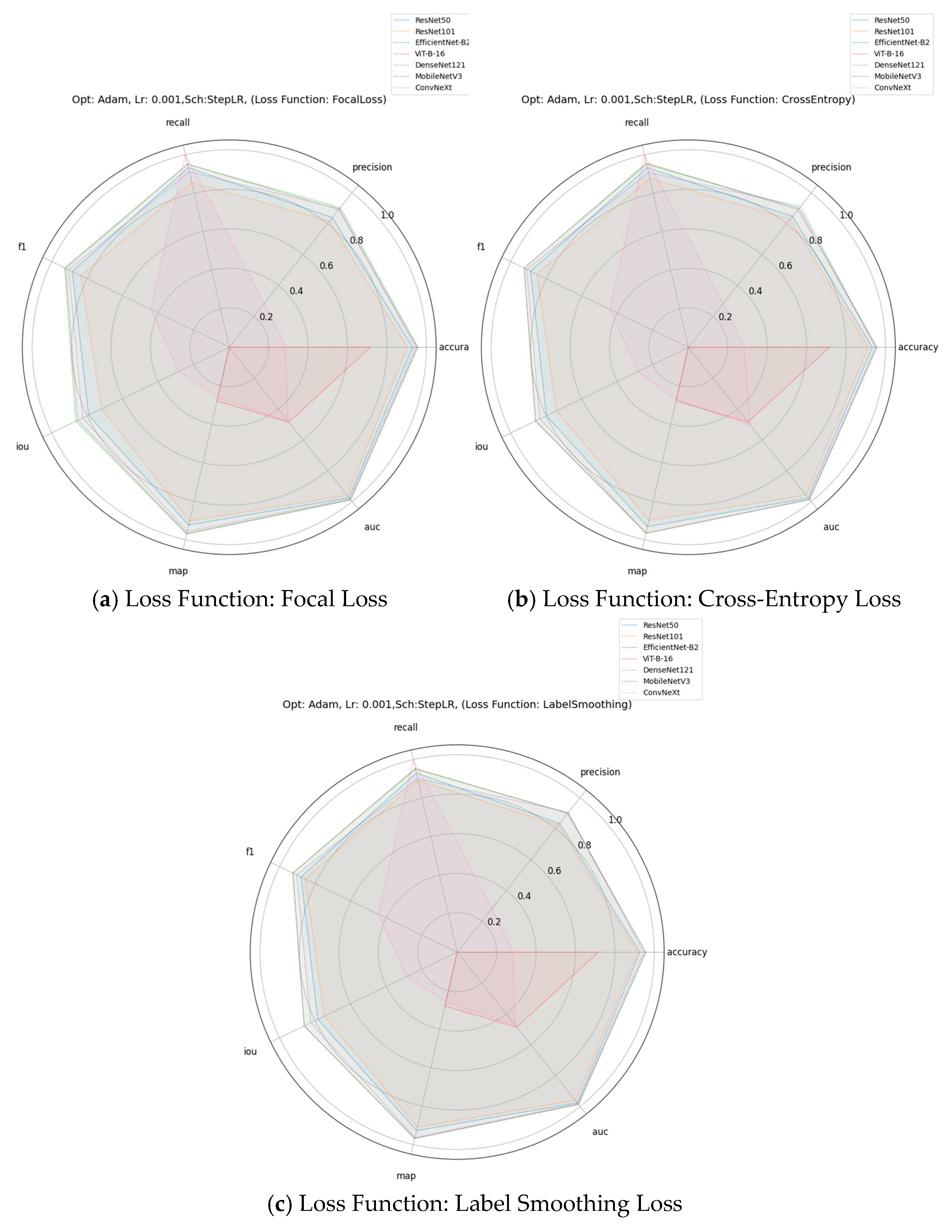
In this study, we investigated the impact of various training parameters on the performance of deep learning models applied to the car collision detection task. The parameters analyzed include learning rates, optimizers, learning rate schedulers, and loss functions. We evaluated their effects on eight key performance metrics: accuracy, precision, recall, F1-score, intersection over union (IoU), mean average precision (mAP), and area under the curve (AUC).

Below are the formal definitions and mathematical formulas of each metric:

3.1. Accuracy

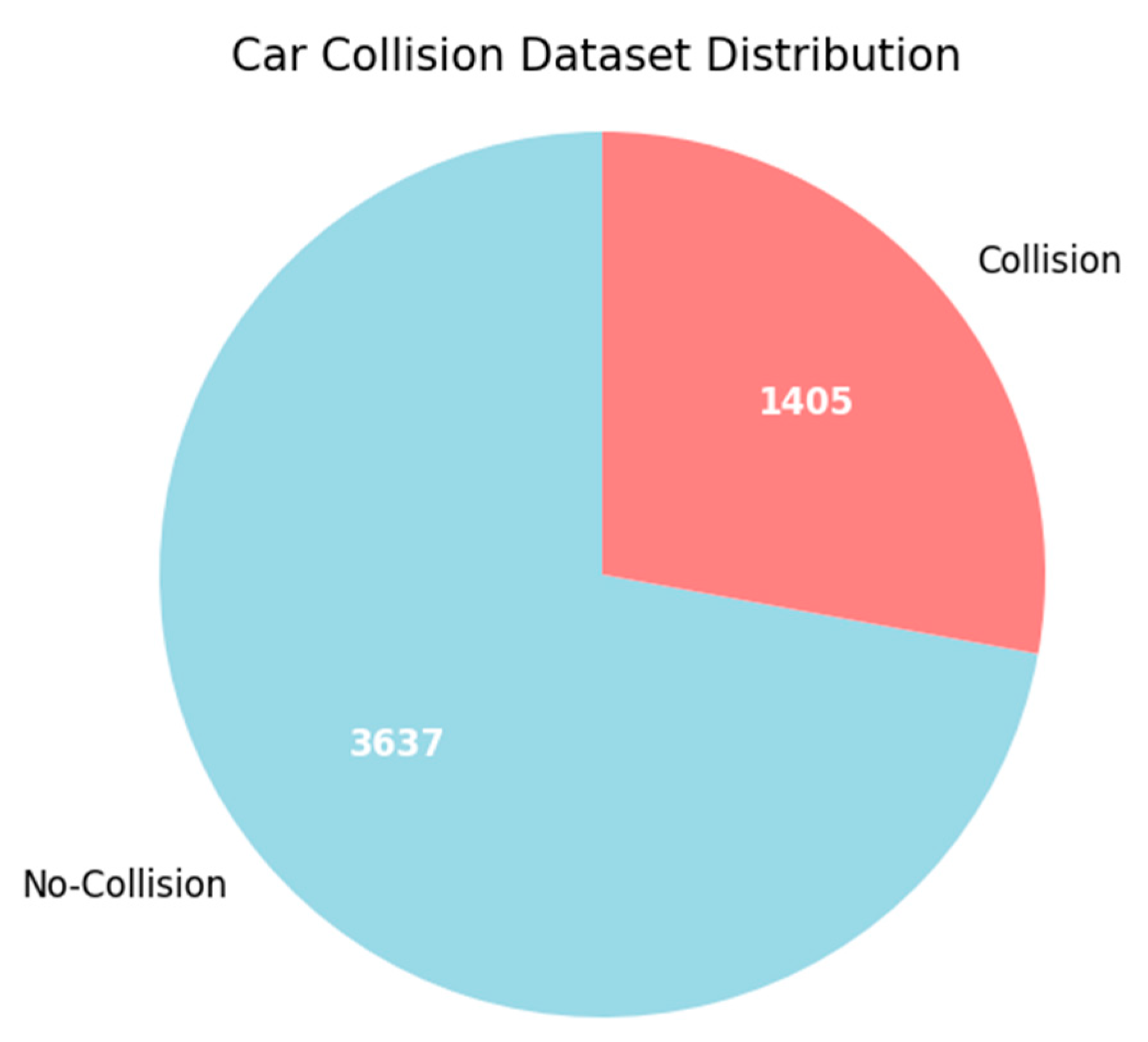
Accuracy is the ratio of correctly predicted instances (both collision and non-collision) to the total instances. It measures overall correctness but may be skewed in imbalanced datasets. While accuracy provides a general measure of performance, it can be misleading in imbalanced datasets (e.g., if collision events are rare). A model predicting mostly non-collisions may still achieve high accuracy without effectively detecting actual collisions.

$$\mathrm{A}\mathrm{c}\mathrm{c}\mathrm{u}\mathrm{r}\mathrm{a}\mathrm{c}\mathrm{y}={\displaystyle \frac{\mathrm{T}\mathrm{P}+\mathrm{T}\mathrm{N}}{\mathrm{T}\mathrm{P}+\mathrm{T}\mathrm{N}+\mathrm{F}\mathrm{P}+\mathrm{F}\mathrm{N}}}$$

(1)

where:

• True Positives (TP) represent cases where the model correctly identifies a collision event, such as accurately detecting an actual vehicle collision.
• True Negatives (TN) indicate instances where the model correctly identifies the absence of a collision, such as confirming no collision in a safe driving scenario.
• False Positives (FP) occur when the model incorrectly predicts a collision when none has occurred.
• False Negatives (FN) denote cases where the model fails to detect an actual collision, such as missing a critical crash event, which could compromise safety.

3.2. Precision

Precision represents the proportion of true collision predictions among all predicted collisions. Precision is critical in minimizing false positives, i.e., incorrectly predicting a collision when there is none. High precision ensures that collision alerts are trustworthy, which is especially important in real-world safety-critical applications to avoid unnecessary emergency responses.

$$\mathrm{P}\mathrm{r}\mathrm{e}\mathrm{c}\mathrm{i}\mathrm{s}\mathrm{i}\mathrm{o}\mathrm{n}={\displaystyle \frac{\mathrm{T}\mathrm{P}}{\mathrm{T}\mathrm{P}+\mathrm{F}\mathrm{P}}}$$

(2)

3.3. Recall

Recall is the proportion of actual collisions correctly identified by the model. Recall is vital in minimizing missed collisions (false negatives). In safety-critical systems, failing to detect a collision is far more dangerous than issuing a false alert, making recall a crucial performance indicator.

$$\mathrm{R}\mathrm{e}\mathrm{c}\mathrm{a}\mathrm{l}\mathrm{l}={\displaystyle \frac{\mathrm{T}\mathrm{P}}{\mathrm{T}\mathrm{P}+\mathrm{F}\mathrm{N}}}$$

(3)

3.4. F1-Score

The F1-score is the harmonic mean of precision and recall, which balances both metrics. The F1-score is particularly useful in imbalanced scenarios, such as collision detection, where one class (non-collision) may dominate. It offers a single measure that balances both precision and recall.

$$\mathrm{F}1=2\times {\displaystyle \frac{\mathrm{P}\mathrm{r}\mathrm{e}\mathrm{c}\mathrm{i}\mathrm{s}\mathrm{i}\mathrm{o}\mathrm{n}\times \mathrm{R}\mathrm{e}\mathrm{c}\mathrm{a}\mathrm{l}\mathrm{l}}{\mathrm{P}\mathrm{r}\mathrm{e}\mathrm{c}\mathrm{i}\mathrm{s}\mathrm{i}\mathrm{o}\mathrm{n}+\mathrm{R}\mathrm{e}\mathrm{c}\mathrm{a}\mathrm{l}\mathrm{l}}}$$

(4)

3.5. Intersection over Union (IoU)

IoU measures the overlap between predicted and ground-truth collision regions, normalized by their union. In binary classification settings, it reduces to comparing predicted collision frames with actual ones. IoU quantifies the accuracy of the model in predicting the location and presence of collision-critical events in space or time. It is particularly useful when spatial localization is required. This quantifies the spatial localization accuracy of collision-critical regions in frames.

$$\mathrm{I}\mathrm{o}\mathrm{U}={\displaystyle \frac{\mathrm{T}\mathrm{P}}{\mathrm{T}\mathrm{P}+\mathrm{F}\mathrm{P}+\mathrm{F}\mathrm{N}}}$$

(5)

3.6. Mean Average Precision (mAP)

mAP is the average of precision values across all recall levels, computed over different confidence thresholds. mAP evaluates how well the model maintains high precision across different levels of recall, giving insight into performance consistency over varying detection thresholds. It is especially useful when predictions are confidence-scored (e.g., collision likelihood).

$$\mathrm{m}\mathrm{A}\mathrm{P}=\underset{0}{\overset{1}{\int }}\mathrm{P}\mathrm{r}\mathrm{e}\mathrm{c}\mathrm{i}\mathrm{s}\mathrm{i}\mathrm{o}\mathrm{n}\left(\mathrm{r}\right)\mathrm{d}\mathrm{r}$$

(6)

3.7. AUC-ROC

AUC represents the area under the Receiver Operating Characteristic (ROC) curve, which plots the True Positive Rate (TPR) against the False Positive Rate (FPR).

AUC-ROC reflects the model’s ability to distinguish between collision and non-collision events. A higher AUC indicates better separability and overall classification capability across all decision thresholds.

$$\mathrm{A}\mathrm{U}\mathrm{C}=\underset{0}{\overset{1}{\int }}\mathrm{T}\mathrm{R}\mathrm{P}\left(\mathrm{f}\right)\mathrm{d}\mathrm{f}$$

(7)

where f = FPR.

All the above evaluation metrics were employed to comprehensively assess the deep learning model’s performance in car collision detection. Accuracy measures overall correctness but may mislead with imbalanced datasets where collisions are rare. Precision minimizes the incorrect prediction of a collision when there is none, while recall ensures all true collisions are detected, which is crucial for safety-critical applications. The F1-score balances precision and recall, offering a single measure of detection efficacy. IoU measures the overlapping between predicted and ground-truth collision regions whereas AUC reflects the model’s ability to distinguish between collision and non-collision events. Together, these metrics provide a robust evaluation framework for this safety-critical application.

4. Results

The performance of seven models, evaluated under various hyperparameter configurations, was assessed under seven key metrics. Figure 4 shows the best-performing model configurations for each metric. The ResNet50 architecture demonstrated superior performance in a majority of the metrics. Specifically, ResNet50 with an AdamW optimizer, a learning rate of 0.0001, CosineAnnealingLR scheduler, and FocalLoss achieved the highest accuracy (0.9782), precision (0.9583), F1-score (0.9617), and IOU (0.9262). A different ResNet50 configuration, utilizing an SGD optimizer, a learning rate of 0.01, CosineAnnealingWarmRestarts scheduler, and CrossEntropy loss, achieved the best AUC (0.9961). Meanwhile, MobileNetV3 with an Adam optimizer, a learning rate of 0.01, StepLR scheduler, and CrossEntropy loss excelled in recall (1.0). Multiple models achieved a recall (1.0), so we used the model which took the least training time, as well as for better comparison. ResNet101 with an SGD optimizer, a learning rate of 0.01, StepLR scheduler, and CrossEntropy loss achieved the highest mAP (0.9921). Overall, ResNet50 emerged as the most effective model, particularly with the AdamW and FocalLoss configuration, underscoring its robustness and versatility across multiple performance metrics.

4.1. Detection Results

For each architecture (seven models), we provided predictions of only the single models that achieved the highest validation accuracy among all of their trained variants. Figure 5 shows the prediction performance of these seven top-performing models, ordered by decreasing accuracy, while Figure 6 shows their corresponding confusion matrices.

4.2. Optimal Configurations for Different Models Across Different Performance Metrics

This section explains the optimal hyperparameter configurations for all the trained models across seven key performance metrics. The best configurations for each metric, identified through extensive hyperparameter tests, are summarized in Table 3, Table 4, Table 5, Table 6, Table 7, Table 8 and Table 9.

4.2.1. Optimal Configurations for Accuracy

Table 3 shows optimal hyperparameter settings that maximize classification accuracy for seven deep learning architectures. Each configuration includes the optimizer, learning rate, scheduler, loss function, and resulting accuracy.

ResNet50 achieves the highest accuracy of 0.978196 using the AdamW optimizer with a learning rate of 0.0001, CosineAnnealingLR scheduler, and FocalLoss. This superior performance stems from AdamW’s adaptive weight decay, which mitigates overfitting by regularizing parameter updates, particularly effective for ResNet50’s deep architecture. FocalLoss enhances generalization by prioritizing hard-to-classify samples and assigning higher weights to misclassified examples. The CosineAnnealingLR scheduler further refines convergence through a smooth, cyclical decay of the learning rate, enabling precise optimization over training epochs.

ResNet101 and EfficientNet-B2 follow with accuracies of 0.975223 and 0.973241, respectively, both leveraging the SGD optimizer with a learning rate of 0.01, StepLR scheduler, and CrossEntropy loss. DenseNet121, using SGD with identical settings, achieves 0.971259, benefiting from its dense connectivity, which enhances feature reuse and gradient flow.

MobileNetV3 secures an accuracy of 0.970268 with SGD (learning rate 0.01), CosineAnnealingLR, and FocalLoss. ConvNeXt attains 0.969277 with Adam (learning rate 0.0001), CosineAnnealingWarmRestarts, and CrossEntropy, where the cyclical learning rate restarts potentially aid in escaping local minima. ViT-B-16, with an accuracy of 0.96333, uses SGD (learning rate 0.001), ReduceLROnPlateau, and CrossEntropy, suggesting that transformer-based models may require adaptive scheduling to optimize performance.

Table 3. Optimal hyperparameter configurations for maximizing classification accuracy across deep learning models.

Model	Optimizer	Learning Rate	Scheduler	Loss Function	Accuracy
ResNet50	AdamW	0.0001	CosineAnnealingLR	FocalLoss	0.978196
ResNet101	SGD	0.01	StepLR	CrossEntropy	0.975223
EfficientNet-B2	SGD	0.01	StepLR	CrossEntropy	0.973241
DenseNet121	SGD	0.01	StepLR	CrossEntropy	0.971259
MobileNetV3	SGD	0.01	CosineAnnealingLR	FocalLoss	0.970268
ConvNeXt	Adam	0.0001	CosineAnnealingWarmRestarts	CrossEntropy	0.969277
ViT-B-16	SGD	0.001	ReduceLROnPlateau	CrossEntropy	0.96333

Table 3. Optimal hyperparameter configurations for maximizing classification accuracy across deep learning models.

Model	Optimizer	Learning Rate	Scheduler	Loss Function	Accuracy
ResNet50	AdamW	0.0001	CosineAnnealingLR	FocalLoss	0.978196
ResNet101	SGD	0.01	StepLR	CrossEntropy	0.975223
EfficientNet-B2	SGD	0.01	StepLR	CrossEntropy	0.973241
DenseNet121	SGD	0.01	StepLR	CrossEntropy	0.971259
MobileNetV3	SGD	0.01	CosineAnnealingLR	FocalLoss	0.970268
ConvNeXt	Adam	0.0001	CosineAnnealingWarmRestarts	CrossEntropy	0.969277
ViT-B-16	SGD	0.001	ReduceLROnPlateau	CrossEntropy	0.96333

4.2.2. Optimal Configurations for Precision

Table 4 outlines the settings that optimize precision, a metric critical for minimizing false positives. Again, ResNet50 leads with a precision of 0.958333, employing AdamW (learning rate 0.0001), CosineAnnealingLR, and FocalLoss. DenseNet121 follows closely at 0.957295 with SGD (learning rate 0.01), StepLR, and CrossEntropy, leveraging its dense connectivity to maintain high precision through efficient feature propagation and momentum-based optimization.

MobileNetV3 achieves 0.947552 using SGD (learning rate 0.01), CosineAnnealingWarmRestarts, and CrossEntropy, where cyclical learning rate adjustments may enhance stability in positive predictions. ResNet101, with 0.945392, reflects DenseNet121’s SGD and StepLR setup with CrossEntropy, benefiting from its depth and periodic learning rate drops. ConvNeXt records 0.939502 with Adam (learning rate 0.0001), ReduceLROnPlateau, and CrossEntropy, where adaptive learning rate reduction stabilizes precision for this modern convolutional architecture.

EfficientNet-B2 and ViT-B-16 yield precisions of 0.938983 and 0.936842, respectively. EfficientNet-B2 uses SGD (learning rate 0.01), CosineAnnealingWarmRestarts, and FocalLoss, suggesting that while cyclical schedules are beneficial, they may introduce variability in precision. ViT-B-16 employs SGD (learning rate 0.001), CosineAnnealingWarmRestarts, and FocalLoss, indicating that transformer models may require further tuning to match convolutional counterparts in precision.

Table 4. Optimal hyperparameter configurations for maximizing precision across deep learning models.

Model	Optimizer	Learning Rate	Scheduler	Loss Function	Precision
ResNet50	AdamW	0.0001	CosineAnnealingLR	FocalLoss	0.958333
DenseNet121	SGD	0.01	StepLR	CrossEntropy	0.957295
MobileNetV3	SGD	0.01	CosineAnnealingWarmRestarts	CrossEntropy	0.947552
ResNet101	SGD	0.01	StepLR	CrossEntropy	0.945392
ConvNeXt	Adam	0.0001	ReduceLROnPlateau	CrossEntropy	0.939502
EfficientNet-B2	SGD	0.01	CosineAnnealingWarmRestarts	FocalLoss	0.938983
ViT-B-16	SGD	0.001	CosineAnnealingWarmRestarts	FocalLoss	0.936842

Table 4. Optimal hyperparameter configurations for maximizing precision across deep learning models.

Model	Optimizer	Learning Rate	Scheduler	Loss Function	Precision
ResNet50	AdamW	0.0001	CosineAnnealingLR	FocalLoss	0.958333
DenseNet121	SGD	0.01	StepLR	CrossEntropy	0.957295
MobileNetV3	SGD	0.01	CosineAnnealingWarmRestarts	CrossEntropy	0.947552
ResNet101	SGD	0.01	StepLR	CrossEntropy	0.945392
ConvNeXt	Adam	0.0001	ReduceLROnPlateau	CrossEntropy	0.939502
EfficientNet-B2	SGD	0.01	CosineAnnealingWarmRestarts	FocalLoss	0.938983
ViT-B-16	SGD	0.001	CosineAnnealingWarmRestarts	FocalLoss	0.936842

4.2.3. Optimal Configurations for Recall

Table 5 details the configurations maximizing recall, a key metric for ensuring all true positives are detected, across the seven models. Recall scores and training times are provided. ConvNeXt, MobileNetV3, and ViT-B-16 achieve perfect recall of 1.0000, using Adam (learning rate 0.01 for ConvNeXt and MobileNetV3, 0.001 for ViT-B-16 with AdamW), StepLR (ConvNeXt and MobileNetV3) or CosineAnnealingWarmRestarts (ViT-B-16), and CrossEntropy (ConvNeXt and MobileNetV3) or LabelSmoothing (ViT-B-16).

EfficientNet-B2 records 0.979021 with Adam (learning rate 0.0001), StepLR, and CrossEntropy, where a lower learning rate ensures cautious weight updates, slightly reducing recall. ResNet101 achieves 0.972028 with Adam (learning rate 0.0001), CosineAnnealingLR, and LabelSmoothing, balancing sensitivity with regularization. ResNet50, at 0.965035, uses SGD (learning rate 0.01), StepLR, and FocalLoss, where FocalLoss’s focus on hard examples may trade off some recall for precision gains.

Table 5. Optimal hyperparameter configurations for maximizing recall across deep learning models.

Model	Optimizer	Learning Rate	Scheduler	Loss Function	Recall	Training Time (s)
MobileNetV3	Adam	0.01	StepLR	CrossEntropy	1	345.73
ConvNeXt	Adam	0.01	StepLR	CrossEntropy	1	697.25
ViT-B-16	AdamW	0.001	CosineAnnealingWarmRestarts	LabelSmoothing	1	1341.91
EfficientNet-B2	Adam	0.0001	StepLR	CrossEntropy	0.979021	1155.55
ResNet101	Adam	0.0001	CosineAnnealingLR	LabelSmoothing	0.972028	1085.43
ResNet50	SGD	0.01	StepLR	FocalLoss	0.965035	1099.19
DenseNet121	SGD	0.001	ReduceLROnPlateau	CrossEntropy	0.958042	646.64

Table 5. Optimal hyperparameter configurations for maximizing recall across deep learning models.

Model	Optimizer	Learning Rate	Scheduler	Loss Function	Recall	Training Time (s)
MobileNetV3	Adam	0.01	StepLR	CrossEntropy	1	345.73
ConvNeXt	Adam	0.01	StepLR	CrossEntropy	1	697.25
ViT-B-16	AdamW	0.001	CosineAnnealingWarmRestarts	LabelSmoothing	1	1341.91
EfficientNet-B2	Adam	0.0001	StepLR	CrossEntropy	0.979021	1155.55
ResNet101	Adam	0.0001	CosineAnnealingLR	LabelSmoothing	0.972028	1085.43
ResNet50	SGD	0.01	StepLR	FocalLoss	0.965035	1099.19
DenseNet121	SGD	0.001	ReduceLROnPlateau	CrossEntropy	0.958042	646.64

4.2.4. Optimal Configurations for F1-Score

Table 6 presents the configurations optimizing the F1-score, and the harmonic mean of precision and recall, offering a balanced performance measure across the seven models. ResNet50 achieved the best F1-score of 0.961672, using AdamW (learning rate 0.0001), CosineAnnealingLR, and FocalLoss. This setup effectively balances its precision (0.958333) and recall (0.965035), with FocalLoss managing the precision-recall trade-off by prioritizing difficult samples. ResNet101 follows with 0.956822, employing SGD (learning rate 0.01), StepLR, and CrossEntropy, leveraging momentum and periodic learning rate adjustments for robust balance in deeper models.

EfficientNet-B2 achieves 0.953688 with an identical SGD setup to ResNet101, demonstrating consistency across scaled architectures. DenseNet121 (0.949033) and MobileNetV3 (0.947917) use SGD (learning rate 0.01) and AdamW (learning rate 0.0001), respectively, with ReduceLROnPlateau and CrossEntropy, where adaptive scheduling fine-tunes their balance. ConvNeXt records 0.946274 with Adam (learning rate 0.0001), CosineAnnealingWarmRestarts, and CrossEntropy, while ViT-B-16, at 0.935428, uses SGD (learning rate 0.001), ReduceLROnPlateau, and CrossEntropy, its lower score reflecting high recall (1.0000) offset by weaker precision (0.936842).

Table 6. Optimal hyperparameter configurations for maximizing F1-score across deep learning models.

Model	Optimizer	Learning Rate	Scheduler	Loss Function	F1
ResNet50	AdamW	0.0001	CosineAnnealingLR	FocalLoss	0.961672
ResNet101	SGD	0.01	StepLR	CrossEntropy	0.956822
EfficientNet-B2	SGD	0.01	StepLR	CrossEntropy	0.953688
DenseNet121	SGD	0.01	ReduceLROnPlateau	CrossEntropy	0.949033
MobileNetV3	AdamW	0.0001	ReduceLROnPlateau	CrossEntropy	0.947917
ConvNeXt	Adam	0.0001	CosineAnnealingWarmRestarts	CrossEntropy	0.946274
ViT-B-16	SGD	0.001	ReduceLROnPlateau	CrossEntropy	0.935428

Table 6. Optimal hyperparameter configurations for maximizing F1-score across deep learning models.

Model	Optimizer	Learning Rate	Scheduler	Loss Function	F1
ResNet50	AdamW	0.0001	CosineAnnealingLR	FocalLoss	0.961672
ResNet101	SGD	0.01	StepLR	CrossEntropy	0.956822
EfficientNet-B2	SGD	0.01	StepLR	CrossEntropy	0.953688
DenseNet121	SGD	0.01	ReduceLROnPlateau	CrossEntropy	0.949033
MobileNetV3	AdamW	0.0001	ReduceLROnPlateau	CrossEntropy	0.947917
ConvNeXt	Adam	0.0001	CosineAnnealingWarmRestarts	CrossEntropy	0.946274
ViT-B-16	SGD	0.001	ReduceLROnPlateau	CrossEntropy	0.935428

4.2.5. Optimal Configurations for Intersection over Union (IoU)

Table 7 showcases the configurations maximizing IoU, a spatial accuracy metric vital for tasks like segmentation, across the seven models.

ResNet50 achieves the highest IoU of 0.926174 with AdamW (learning rate 0.0001), CosineAnnealingLR, and FocalLoss, extending its versatility to spatial tasks. This configuration’s success likely stems from FocalLoss’s focus on precise boundary predictions and CosineAnnealingLR’s smooth optimization. ResNet101 (0.917219) and EfficientNet-B2 (0.911475) use SGD (learning rate 0.01), StepLR, and CrossEntropy, leveraging depth and scaling with momentum-driven stability.

DenseNet121 (0.90301) and MobileNetV3 (0.90099) employ SGD (learning rate 0.01) and AdamW (learning rate 0.0001), respectively, with ReduceLROnPlateau and CrossEntropy, where adaptive scheduling enhances spatial consistency. ConvNeXt (0.898026) uses Adam (learning rate 0.0001), CosineAnnealingWarmRestarts, and CrossEntropy, while ViT-B-16 (0.878689) relies on SGD (learning rate 0.001), ReduceLROnPlateau, and CrossEntropy, its lower IoU reflecting transformer challenges in spatial reasoning compared to convolutional models.

Table 7. Optimal hyperparameter configurations for maximizing intersection over union (IoU) across deep learning models.

Model	Optimizer	Learning Rate	Scheduler	Loss Function	IOU
ResNet50	AdamW	0.0001	CosineAnnealingLR	FocalLoss	0.926174
ResNet101	SGD	0.01	StepLR	CrossEntropy	0.917219
EfficientNet-B2	SGD	0.01	StepLR	CrossEntropy	0.911475
DenseNet121	SGD	0.01	ReduceLROnPlateau	CrossEntropy	0.90301
MobileNetV3	AdamW	0.0001	ReduceLROnPlateau	CrossEntropy	0.90099
ConvNeXt	Adam	0.0001	CosineAnnealingWarmRestarts	CrossEntropy	0.898026
ViT-B-16	SGD	0.001	ReduceLROnPlateau	CrossEntropy	0.878689

Table 7. Optimal hyperparameter configurations for maximizing intersection over union (IoU) across deep learning models.

Model	Optimizer	Learning Rate	Scheduler	Loss Function	IOU
ResNet50	AdamW	0.0001	CosineAnnealingLR	FocalLoss	0.926174
ResNet101	SGD	0.01	StepLR	CrossEntropy	0.917219
EfficientNet-B2	SGD	0.01	StepLR	CrossEntropy	0.911475
DenseNet121	SGD	0.01	ReduceLROnPlateau	CrossEntropy	0.90301
MobileNetV3	AdamW	0.0001	ReduceLROnPlateau	CrossEntropy	0.90099
ConvNeXt	Adam	0.0001	CosineAnnealingWarmRestarts	CrossEntropy	0.898026
ViT-B-16	SGD	0.001	ReduceLROnPlateau	CrossEntropy	0.878689

4.2.6. Optimal Configurations for Mean Average Precision (mAP)

Table 8 shows the configurations optimizing mAP, a detection metric that averages precision across recall levels, for the seven models. ResNet101 leads with a mAP of 0.992104 using SGD (learning rate 0.01), StepLR, and CrossEntropy, its depth capturing intricate features for detection, stabilized by momentum and periodic learning rate drops. ResNet50 follows at 0.991379 with SGD (learning rate 0.01), CosineAnnealingWarmRestarts, and CrossEntropy, where cyclical learning enhances generalization. DenseNet121 achieves 0.989826 with SGD (learning rate 0.01), CosineAnnealingWarmRestarts, and FocalLoss, leveraging FocalLoss to address hard examples.

EfficientNet-B2 (0.989524) uses AdamW (learning rate 0.0001), StepLR, and LabelSmoothing, combining adaptive optimization with regularization. ConvNeXt (0.986675) and ViT-B-16 (0.985686) employ SGD (learning rate 0.001) with CosineAnnealingLR and ReduceLROnPlateau, respectively, and LabelSmoothing, suggesting regularization aids modern architectures. MobileNetV3 (0.98276) uses SGD (learning rate 0.01), StepLR, and CrossEntropy, performing competitively despite its lightweight design.

mAP scores cluster tightly between 0.98276 and 0.992104, indicating robust detection capabilities across models, with convolutional models slightly ahead of transformers.

Table 8. Optimal hyperparameter configurations for maximizing mean average precision (mAP) across deep learning models.

Model	Optimizer	Learning Rate	Scheduler	Loss Function	mAP
ResNet101	SGD	0.01	StepLR	CrossEntropy	0.992104
ResNet50	SGD	0.01	CosineAnnealingWarmRestarts	CrossEntropy	0.991379
DenseNet121	SGD	0.01	CosineAnnealingWarmRestarts	FocalLoss	0.989826
EfficientNet-B2	AdamW	0.0001	StepLR	LabelSmoothing	0.989524
ConvNeXt	SGD	0.001	CosineAnnealingLR	LabelSmoothing	0.986675
ViT-B-16	SGD	0.001	ReduceLROnPlateau	LabelSmoothing	0.985686
MobileNetV3	SGD	0.01	StepLR	CrossEntropy	0.98276

Table 8. Optimal hyperparameter configurations for maximizing mean average precision (mAP) across deep learning models.

Model	Optimizer	Learning Rate	Scheduler	Loss Function	mAP
ResNet101	SGD	0.01	StepLR	CrossEntropy	0.992104
ResNet50	SGD	0.01	CosineAnnealingWarmRestarts	CrossEntropy	0.991379
DenseNet121	SGD	0.01	CosineAnnealingWarmRestarts	FocalLoss	0.989826
EfficientNet-B2	AdamW	0.0001	StepLR	LabelSmoothing	0.989524
ConvNeXt	SGD	0.001	CosineAnnealingLR	LabelSmoothing	0.986675
ViT-B-16	SGD	0.001	ReduceLROnPlateau	LabelSmoothing	0.985686
MobileNetV3	SGD	0.01	StepLR	CrossEntropy	0.98276

4.2.7. Optimal Configurations for Area Under the ROC Curve (AUC)

Table 9 presents the configurations maximizing AUC. ResNet50 achieves the highest AUC of 0.996138 with SGD (learning rate 0.01), CosineAnnealingWarmRestarts, and CrossEntropy, where cyclical learning enhances class separation. ResNet101 follows at 0.995715 with SGD (learning rate 0.01), StepLR, and CrossEntropy, ensuring stable optimization. EfficientNet-B2 (0.995261) uses AdamW (learning rate 0.0001), StepLR, and LabelSmoothing, benefiting from adaptive regularization.

DenseNet121 (0.995232) employs SGD (learning rate 0.01), CosineAnnealingLR, and CrossEntropy, with smooth learning rate decay aiding discrimination. ConvNeXt (0.99426) and ViT-B-16 (0.993844) use SGD (learning rate 0.001) with CosineAnnealingLR and StepLR, respectively, and LabelSmoothing or CrossEntropy, while MobileNetV3 (0.993534) mirrors ResNet101’s SGD setup.

Table 9. Optimal hyperparameter configurations for maximizing area under the ROC curve (AUC) across deep learning models.

Model	Optimizer	Learning Rate	Scheduler	Loss Function	AUC
ResNet50	SGD	0.01	CosineAnnealingWarmRestarts	CrossEntropy	0.996138
ResNet101	SGD	0.01	StepLR	CrossEntropy	0.995715
EfficientNet-B2	AdamW	0.0001	StepLR	LabelSmoothing	0.995261
DenseNet121	SGD	0.01	CosineAnnealingLR	CrossEntropy	0.995232
ConvNeXt	SGD	0.001	CosineAnnealingLR	LabelSmoothing	0.99426
ViT-B-16	SGD	0.001	StepLR	CrossEntropy	0.993844
MobileNetV3	SGD	0.01	StepLR	CrossEntropy	0.993534

Table 9. Optimal hyperparameter configurations for maximizing area under the ROC curve (AUC) across deep learning models.

Model	Optimizer	Learning Rate	Scheduler	Loss Function	AUC
ResNet50	SGD	0.01	CosineAnnealingWarmRestarts	CrossEntropy	0.996138
ResNet101	SGD	0.01	StepLR	CrossEntropy	0.995715
EfficientNet-B2	AdamW	0.0001	StepLR	LabelSmoothing	0.995261
DenseNet121	SGD	0.01	CosineAnnealingLR	CrossEntropy	0.995232
ConvNeXt	SGD	0.001	CosineAnnealingLR	LabelSmoothing	0.99426
ViT-B-16	SGD	0.001	StepLR	CrossEntropy	0.993844
MobileNetV3	SGD	0.01	StepLR	CrossEntropy	0.993534

5. Discussion

To understand how different hyperparameters affect the performance of different models, we organized models trained under the same settings into groups, changing just one hyperparameter at a time. For example, to explore the impact of learning rates, we grouped all the trained models with varying learning rates while keeping all other hyperparameters the same. From each group of the same models, we picked the model with the highest accuracy to identify the best learning rate. We applied this same method to other hyperparameters as well, systematically testing their effects to see how each tested hyperparameter influences the model’s ability to make accurate predictions. The following section explains the impact of each parameter separately.

5.1. Impact of Learning Optimizers

The choice of optimizer significantly influences the training dynamics and performance of deep learning models. Optimizers such as SGD, Adam, and AdamW each employ distinct strategies for navigating the loss landscape, impacting metrics. SGD (Figure 7c) consistently delivers superior performance across models like ResNet101 and EfficientNet-B2, leveraging momentum to achieve high accuracy and robust generalization. In contrast, Adam and AdamW, which use adaptive learning rates, often underperform with certain architectures (e.g., ViT-B-16 and ConvNeXt) under the given hyperparameters, resulting in lower accuracy and poor convergence. The radar graphs (Figure 7a–c) generated for each optimizer visually illustrate these effects, comparing the performance of the best models across the evaluated metrics, and highlighting the strengths and limitations of each optimizer in optimizing diverse model architectures.

5.2. Impact of Learning Rate Schedulers

The choice of learning rate scheduler significantly influences the performance of deep learning models by controlling how the learning rate adapts during training, thereby affecting convergence and generalization. Each scheduler offers distinct strategies for adjusting the learning rate, impacting performance metrics. For instance, CosineAnnealingWarmRestarts often facilitates better exploration of the loss landscape through periodic learning rate restarts, potentially leading to improved performance, as evidenced by the superior accuracy of ResNet50 under this scheduler. Conversely, StepLR’s fixed step reductions may result in suboptimal convergence if not carefully tuned. The radar graphs (Figure 8a–d) generated for each scheduler visually demonstrate these effects, highlighting the comparative performance of the best models across the evaluated metrics, with each graph showcasing the strengths and trade-offs induced by the respective scheduling strategy.

5.3. Impact of Learning Rates

The learning rate plays a critical role in determining the convergence and performance of deep learning models by controlling the step size of parameter updates during optimization. Different learning rates can lead to varying results in terms of model performance metrics. A high learning rate (e.g., 0.01) may cause instability or failure to converge, as seen in the poor performance of models like ViT-B-16 and ConvNeXt, while a lower learning rate (e.g., 0.0001) often facilitates stable convergence and higher performance, as evidenced by ResNet50’s superior accuracy. The radar graphs (Figure 9a–c) generated for each learning rate visually illustrate these effects, comparing the performance of the best models across the evaluated metrics, highlighting the trade-offs and optimal configurations induced by different learning rate settings.

5.4. Impact of Loss Functions

The choice of loss function significantly influences the training dynamics and performance of deep learning models by shaping the optimization objective, thereby affecting convergence and generalization across various metrics. Each loss function addresses different aspects of class imbalance and model confidence. For instance, FocalLoss, designed to focus on hard-to-classify examples, slightly enhances performance for models like EfficientNet-B2, as evidenced by its higher accuracy and mAP. Conversely, CrossEntropy and LabelSmoothing yield comparable results for most models, though LabelSmoothing may improve generalization by reducing overconfidence, as seen in MobileNetV3’s balanced metrics. However, models like ViT-B-16 and ConvNeXt exhibit poor performance across all loss functions. The radar graphs (Figure 10a–c) generated for each loss function visually illustrate these effects, comparing the performance of the best models across the evaluated metrics, and highlighting the trade-offs and effectiveness of each loss function in optimizing diverse model architectures.

6. Conclusions

In this paper, we evaluated seven pre-trained deep learning models for car collision detection using dashcam images. In our experimental settings all models were evaluated on seven performance metrics under various hyperparameter settings (Table 1), with a total of 756 hyperparameter configurations tested for this study. ResNet50, optimized with AdamW, a learning rate of 0.0001, CosineAnnealingLR scheduler, and Focal Loss, emerged as the top performer, achieving an accuracy of 0.9782, F1-score of 0.9617, and IoU of 0.9262. These results highlight the efficacy of transfer learning and the critical role of hyperparameter tuning in enhancing model performance. SGD-based configurations often outperform adaptive optimizers in accuracy and localization.

7. Limitations and Future Work

In this paper, we evaluated the models for car collision detection using only static frames. In the future, we will incorporate temporal video sequences to improve car collision detection robustness and assess the generalization of the models under temporal settings. Additionally, for practical deployment, we will evaluate the models’ performance on real-time video streams, optimizing for low latency and ensuring they can handle the demands of live processing. Furthermore, we will create a larger and more diverse dataset by incorporating more videos, improving the models’ ability to handle varied scenarios. Moreover, we will explore the impact of additional hyperparameters and settings, including batch size, weight decay, momentum, advanced data augmentation techniques, and input resolution, to further enhance model performance and robustness.

References

1. World Health Organization. Global Status Report on Road Safety 2023; World Health Organization: Geneva, Switzerland, 2023. Available online: https://iris.who.int/bitstream/handle/10665/375016/9789240086517-eng.pdf?sequence=1 (accessed on 5 June 2025).
2. Rezaei, Z.; Ebrahimpour-Komleh, H. Prediction and detection of car accidents in video by deep learning. In Proceedings of the 2021 5th International Conference on Pattern Recognition and Image Analysis (IPRIA), Kashan, Iran, 28–29 April 2021; IEEE: New York, NY, USA, 2021; pp. 1–9. [Google Scholar]
3. National Safety Council (NSC). Motor Vehicle—Type of Crash. Available online: https://injuryfacts.nsc.org/motor-vehicle/overview/type-of-crash/ (accessed on 14 June 2025).
4. Carrodano, C. Data-driven risk analysis of nonlinear factor interactions in road safety using Bayesian networks. Sci. Rep. 2024, 14, 18948. [Google Scholar] [CrossRef] [PubMed]
5. He, M.; Meng, G.; Wu, X.; Han, X.; Fan, J. Road Traffic Accident Prediction Based on Multi-Source Data—A Systematic Review. Promet-Traffic Transp. 2025, 37, 499–522. [Google Scholar] [CrossRef]
6. Wu, K.; Li, W.; Xiao, X. AccidentGPT: Large multi-modal foundation model for traffic accident analysis. arXiv 2024, arXiv:2401.03040. [Google Scholar]
7. Kolte, N.; Mittal, S.K. ERDMS: Bridging the Gap Between Accident Detection and Timely Medical Assistance. In Proceedings of the 2024 Asia Pacific Conference on Innovation in Technology (APCIT), Mysore, India, 26–27 July 2024; IEEE: New York, NY, USA, 2024; pp. 1–8. [Google Scholar]
8. Wang, Z.; Zhan, J.; Duan, C.; Guan, X.; Lu, P.; Yang, K. A review of vehicle detection techniques for intelligent vehicles. IEEE Trans. Neural Netw. Learn. Syst. 2022, 34, 3811–3831. [Google Scholar] [CrossRef] [PubMed]
9. Sang, J.; Wu, J.; Guo, P.; Hu, H.; Xiang, H.; Zhang, Q.; Cai, B. An improved YOLOv2 for vehicle detection. Sensors 2018, 18, 4272. [Google Scholar] [CrossRef] [PubMed]
10. Li, X.; Mohammed, R.; Mangin, T.; Saha, S.; Kelly, K.; Whitaker, R.; Tasdizen, T. Joint audio-visual idling vehicle detection with streamlined input dependencies. In Proceedings of the Winter Conference on Applications of Computer Vision, Tucson, AZ, USA, 28 February–4 March 2025; pp. 885–894. [Google Scholar]
11. Gautham, B.; Sangeetha, K. Real-Time Pedestrian Detection and Tracking in Dynamic Urban Environments Using YOLO for Intelligent Video Systems. In Proceedings of the 2025 3rd International Conference on Intelligent Systems, Advanced Computing and Communication (ISACC), Silchar, India, 27–28 February 2025; IEEE: New York, NY, USA, 2025; pp. 128–133. [Google Scholar]
12. Luo, X.; Li, X.; Goh, Y.M.; Song, X.; Liu, Q. Application of machine learning technology for occupational accident severity prediction in the case of construction collapse accidents. Saf. Sci. 2023, 163, 106138. [Google Scholar] [CrossRef]
13. Rahim, M.A.; Hassan, H.M. A deep learning based traffic crash severity prediction framework. Accid. Anal. Prev. 2021, 154, 106090. [Google Scholar] [CrossRef] [PubMed]
14. Yang, Z.; Zhang, W.; Feng, J. Predicting multiple types of traffic accident severity with explanations: A multi-task deep learning framework. Saf. Sci. 2022, 146, 105522. [Google Scholar] [CrossRef]
15. Zhou, Z. Attention based stack resnet for citywide traffic accident prediction. In Proceedings of the 2019 20th IEEE International Conference on Mobile Data Management (MDM), Hong Kong, China, 10–13 June 2019; IEEE: New York, NY, USA, 2019; pp. 369–370. [Google Scholar]
16. Jaspin, K.; Bright, A.A.; Legin, M.L. Accident Detection and Severity Classification System using YOLO Model. In Proceedings of the 2024 3rd International Conference on Applied Artificial Intelligence and Computing (ICAAIC), Salem, India, 5–7 June 2024; IEEE: New York, NY, USA, 2024; pp. 1160–1167. [Google Scholar]
17. Banerjee, S.; Mondal, M.K.; Roy, M.; Alnumay, W.S.; Biswas, U. A Deep Learning-based Car Accident Detection Framework using Edge and Cloud Computing. IEEE Access 2024, 12, 130107–130115. [Google Scholar] [CrossRef]
18. Huang, X.; He, P.; Rangarajan, A.; Ranka, S. Intelligent intersection: Two-stream convolutional networks for real-time near-accident detection in traffic video. ACM Trans. Spat. Algorithms Syst. 2020, 6, 1–28. [Google Scholar] [CrossRef]
19. Le, T.-N.; Ono, S.; Sugimoto, A.; Kawasaki, H. Attention R-CNN for accident detection. In Proceedings of the 2020 IEEE Intelligent Vehicles Symposium (IV), Las Vegas, NV, USA, 19 October–13 November 2020; IEEE: New York, NY, USA, 2020; pp. 313–320. [Google Scholar]
20. Javed, R.; Mazhar, T.; Aoun, M.; Shahzad, T.; Al-AlShaikh, H.A.; Ghadi, Y.Y.; Saudagar, A.K.; Khan, M.A. Deep Learning and IoT-Enabled Accident Detection and Reporting for Smart Cities Domain. KSII Trans. Internet Inf. Syst. 2025, 19, 1140–1166. [Google Scholar]
21. Amrouche, A.; Kebir, S.T. Enhancing Road Safety: Car Crash Detection (CCD) Using CNN Model. In Proceedings of the 2024 International Conference on Telecommunications and Intelligent Systems (ICTIS), Djelfa, Algeria, 14–15 December 2024; IEEE: New York, NY, USA, 2024; pp. 1–6. [Google Scholar]
22. Praveen, R.V.S.; Raju, A.; Anjana, P.; Shibi, B. IoT and ML for Real-Time Vehicle Accident Detection Using Adaptive Random Forest. In Proceedings of the 2024 Global Conference on Communications and Information Technologies (GCCIT), Bangalore, India, 25–26 October 2024; IEEE: New York, NY, USA, 2024; pp. 1–5. [Google Scholar]
23. Hosna, A.; Merry, E.; Gyalmo, J.; Alom, Z.; Aung, Z.; Azim, M.A. Transfer learning: A friendly introduction. J. Big Data 2022, 9, 102. [Google Scholar] [CrossRef] [PubMed]
24. Ayana, G.; Dese, K.; Choe, S. Transfer learning in breast cancer diagnoses via ultrasound imaging. Cancers 2021, 13, 738. [Google Scholar] [CrossRef] [PubMed]
25. Benítez-Andrades, J.A.; Prada-García, C.; Ordás-Reyes, N.; Blanco, M.E.; Merayo, A.; Serrano-García, A. Enhanced prediction of spine surgery outcomes using advanced machine learning techniques and oversampling methods. Health Inf. Sci. Syst. 2025, 13, 24. [Google Scholar] [CrossRef] [PubMed]
26. Lin, T.-Y.; Goyal, P.; Girshick, R.; He, K.; Dollár, P. Focal loss for dense object detection. In Proceedings of the IEEE International Conference on Computer Vision, Venice, Italy, 22–29 October 2017; pp. 2980–2988. [Google Scholar]
27. Peng, H.; Wu, C.; Xiao, Y. CBF-IDS: Addressing class imbalance using CNN-BiLSTM with focal loss in network intrusion detection system. Appl. Sci. 2023, 13, 11629. [Google Scholar] [CrossRef]
28. Ju, L.; Wang, X.; Wang, L.; Mahapatra, D.; Zhao, X.; Zhou, Q.; Liu, T.; Ge, Z. Improving medical images classification with label noise using dual-uncertainty estimation. IEEE Trans. Med. Imaging 2022, 41, 1533–1546. [Google Scholar] [CrossRef] [PubMed]
29. Loshchilov, I.; Hutter, F. Sgdr: Stochastic gradient descent with warm restarts. arXiv 2016, arXiv:1608.03983. [Google Scholar]
Figure 1. The basic flow of the proposed car collision detection system.
Applsci 15 07001 g001
Figure 2. Data distribution used in our car collision detection system.
Applsci 15 07001 g002
Figure 3. Illustration of configuration settings.
Applsci 15 07001 g003
Figure 4. The bar graph shows the best model for each metric. There was no model in our experiments that achieved the best results on each metric. Resnet50 (AdamW, 0.0001, StepLR, CrossEntropy) performed best on four metrics (accuracy, precision, F1-score, IOU).
Applsci 15 07001 g004
Figure 5. Comparative visualization of “collision” and “non-collision” prediction results from the seven top-performing models, each selected as the highest-accuracy variant of its respective architecture, under their optimal configurations.
Applsci 15 07001 g005aApplsci 15 07001 g005b
Figure 6. Confusion matrices for the seven top-performing models, each selected as the highest-accuracy variant of its architecture, displaying true versus predicted “collision” and “non-collision” classifications, ordered by decreasing accuracy. (a) ResNet50 (AdamW, 0.0001, CosineAnnealingLR, FocalLoss); (b) ResNet101 (SGD, 0.01, StepLR, CrossEntropy); (c) Efficient-B2 (SGD, 0.01, StepLR, CrossEntropy); (d) Desnet (SGD, 0.01, StepLR, CrossEntropy); (e) MobileNet (SGD, 0.01, CosineAnnealingLR, FocalLoss); (f) ConvexNet (Adam, 0.0001, CosineAnnealingWarmRestarts, CrossEntropy); (g) ViT-B16 (SGD, 0.001, ReduceLROnPlateau, CrossEntropy).
Applsci 15 07001 g006
Figure 7. Radar graph comparing model performance across different optimizers for the car collision detection system while keeping LR, loss, and schedulers the same.
Applsci 15 07001 g007
Figure 8. Radar graph comparing model performance across different schedulers for the car collision detection system while keeping LR, loss, and optimizer the same.
Applsci 15 07001 g008
Figure 9. Radar graph comparing model performance across different learning rates for the car collision detection system while keeping schedulers, loss, and optimizer the same.
Applsci 15 07001 g009
Figure 10. Radar graph comparing model performance across different loss functions for the car collision detection system while keeping LR, optimizer, and scheduler the same.
Applsci 15 07001 g010