Path Planning of Underground Robots via Improved A* and Dynamic Window Approach

Abstract

This paper addresses the limitations of the A* algorithm in underground roadway path planning, such as proximity to roadway boundaries, intersection with obstacle corners, trajectory smoothness, and timely obstacle avoidance (e.g., fallen rocks, miners, and moving equipment). To overcome these challenges, we propose an improved path planning algorithm integrating an enhanced A* method with an improved Dynamic Window Approach (DWA). First, a diagonal collision detection mechanism is implemented within the A* algorithm to effectively avoid crossing obstacle corners, thus enhancing path safety. Secondly, roadway width is incorporated into the heuristic function to guide paths toward the roadway center, improving stability and feasibility. Subsequently, based on multiple global path characteristics—including path length, average curvature, fluctuation degree, and direction change rate—an adaptive B-spline curve smoothing method generates smoother paths tailored to the robot’s kinematic requirements. Furthermore, the global path is segmented into local reference points for DWA, ensuring seamless integration of global and local path planning. To prevent local optimization traps during obstacle avoidance, a distance-based cost function is introduced into DWA’s evaluation criteria, maintaining alignment with the global path. Experimental results demonstrate that the proposed method significantly reduces node expansions by 43.79%, computation time by 16.28%, and path inflection points by 80.70%. The resultant path is smoother, centered within roadways, and capable of effectively avoiding dynamic and static obstacles, thereby ensuring the safety and efficiency of underground robotic transport operations.

1. Introduction

As the demand for robotic applications continues to grow in modern society, intelligent technologies have been widely applied across various fields, particularly in the mining industry. With the introduction of the concept of smart mining, various types of robots have gradually been deployed in underground roadways. However, due to the complex and variable width of underground roadways, the conditions for robot movement differ, making the path planning of underground mobile robots particularly crucial.

The path planning of mobile robots is a complex but crucial task. Its core goal is to find an optimal and collision-free path from the starting point to the target point for the robot in two-dimensional or three-dimensional space [1,2]. In this process, the robot needs to make motion decisions based on objective functions (such as the shortest path, the shortest time, the least resource cost, etc.). According to the perception of environmental information, path planning is divided into two categories: global path planning and local path planning [3]. Local path planning algorithms include the artificial potential field method [4], simulated annealing method [5], dynamic window method [6], neural network [7], and reinforcement learning [8]. Global path planning algorithms include the Dijkstra algorithm [9], RRT algorithm [10], D* algorithm [11], A* algorithm [12], and so on. The A* algorithm is widely used because of its simple calculation and efficient generation of the shortest path. However, the A* algorithm has problems such as long search time, low efficiency, and uneven path.

Many scholars, both domestically and internationally, have proposed various improvement strategies to address the limitations of the A* algorithm. Zhang [13] effectively reduced the turning frequency of the path by introducing the angle evaluation mechanism into the heuristic function, but also significantly increased the burden of node calculation. A bidirectional A* algorithm combining four-domain and eight-neighborhood search mechanisms was developed by Fang [14]. This algorithm significantly shortens the search time, but it is easy to fall into a local optimal solution. Kong [15] optimized the cost function of the bidirectional A* algorithm by introducing a weight coefficient, which can generate the shortest path, but there are too many inflection points in the path, which is not conducive to the smooth driving of the mobile robot. Zhang [16] developed an A* algorithm integrated with jump point search, achieving memory reduction through long-distance jumps. However, excessive unnecessary jump point searches could potentially degrade search efficiency. Lai [17] introduced a dynamic weighting factor in the heuristic function, adjusted the search neighborhood range, and reduced the number of search nodes, thereby improving the efficiency of the algorithm. Yu [18] extended the search direction of eight neighborhoods to twelve neighborhoods to reduce the number of nodes in the search process of the bidirectional A* algorithm. Chen [19] improved the traditional eight-neighborhood search to a five-neighborhood search, which effectively reduced the traversal of irrelevant points and significantly improved the path search efficiency. Chen [20] proposed an improved bidirectional A* algorithm, adding local path constraints to the search path, and introducing a cubic B-spline curve to smooth the inflection point, which successfully solved the problem of diagonal collision and non-smooth path. Implementing map inflation preprocessing, Li [21] developed an obstacle-avoidance strategy that effectively eliminates path–obstacle intersections through geometric constraint transformation of environmental configuration space. Wang [22] proposed a path-smoothing strategy to reduce the redundant points in the path planned by the bidirectional A* algorithm (B-A*).

However, the above algorithm cannot achieve local obstacle avoidance. Therefore, in recent years, scholars have often combined global path planning with local path planning. A novel path planning method combining improved A* algorithm and dynamic window approach (DWA) was developed by Wang [23] for legged robots operating in coal mine environments. On the premise of ensuring the safety and stability of robot walking, compared with the traditional A* algorithm, this method not only shortens the calculation time, but also reduces the path length and makes the path smoother. By combining these two algorithms, the global path planning ability is further enhanced, so that the robot can effectively avoid dynamic and static obstacles in a multi-obstacle environment. Zhang [24] developed an improved A*-DWA fusion algorithm, which optimizes the path of mobile robots through real-time dynamic obstacle avoidance to ensure that the planned path is safe and efficient, and has good smoothness. Guo [25] introduced a path planning method combining an improved Dijkstra algorithm and DWA. This method can maintain the smooth speed and smooth trajectory of the robot when facing static and dynamic obstacles. At the same time, the angular velocity fluctuation is small, which proves the stability of the robot motion and the ability to adjust the direction in real time, and has a good obstacle avoidance effect.

To address the issues in the A* algorithm for underground roadway path planning, such as diagonal movement collisions at corner points, proximity to roadway edges, and unsmooth paths, this paper proposes the following improvements. First, a crossing point detection mechanism is introduced during diagonal movements to prevent collisions when the path crosses obstacle corners. Second, roadway width information is integrated into the heuristic function, enabling the planned path to avoid narrow areas, thereby improving the path quality and ensuring safe navigation. Additionally, based on the global path features planned by the A* algorithm, an appropriate B-spline curve order and smoothing factor are selected to achieve a smooth transition of the path. For local obstacle avoidance, the smoothed global path is divided into multiple sub-goals, with the DWA algorithm using these sub-goals as local targets for obstacle avoidance. To prevent excessive deviation from the global path during obstacle avoidance, a distance cost function is added to the evaluation function of the DWA algorithm. Finally, experiments demonstrate that the improved adaptive A* algorithm is able to plan a path closely following the center of the roadway, avoid collisions during diagonal movement, generate smooth paths without sharp turns, and effectively avoid newly introduced static and dynamic obstacles. Experimental results show that the proposed method significantly enhances the feasibility and safety of path planning.

The following of this paper is organized as follows:

Section 2 systematically presents the classical A* algorithm and proposes targeted improvements to overcome its shortcomings in underground roadway path-planning scenarios.

Section 3 first reviews the fundamentals of the Dynamic Window Approach (DWA) and then introduces specific enhancements; building on this, it puts forward a global–local cooperative scheme that fuses the improved A* with the refined DWA and explains its working mechanism.

Section 4 validates, through experiments and comparative analyses, the efficacy and superiority of both the improved A* algorithm and the integrated improved A*–DWA algorithm.

Section 5 concludes the work.

2. Improved A* Algorithm

2.1. The Principle of A* Algorithm

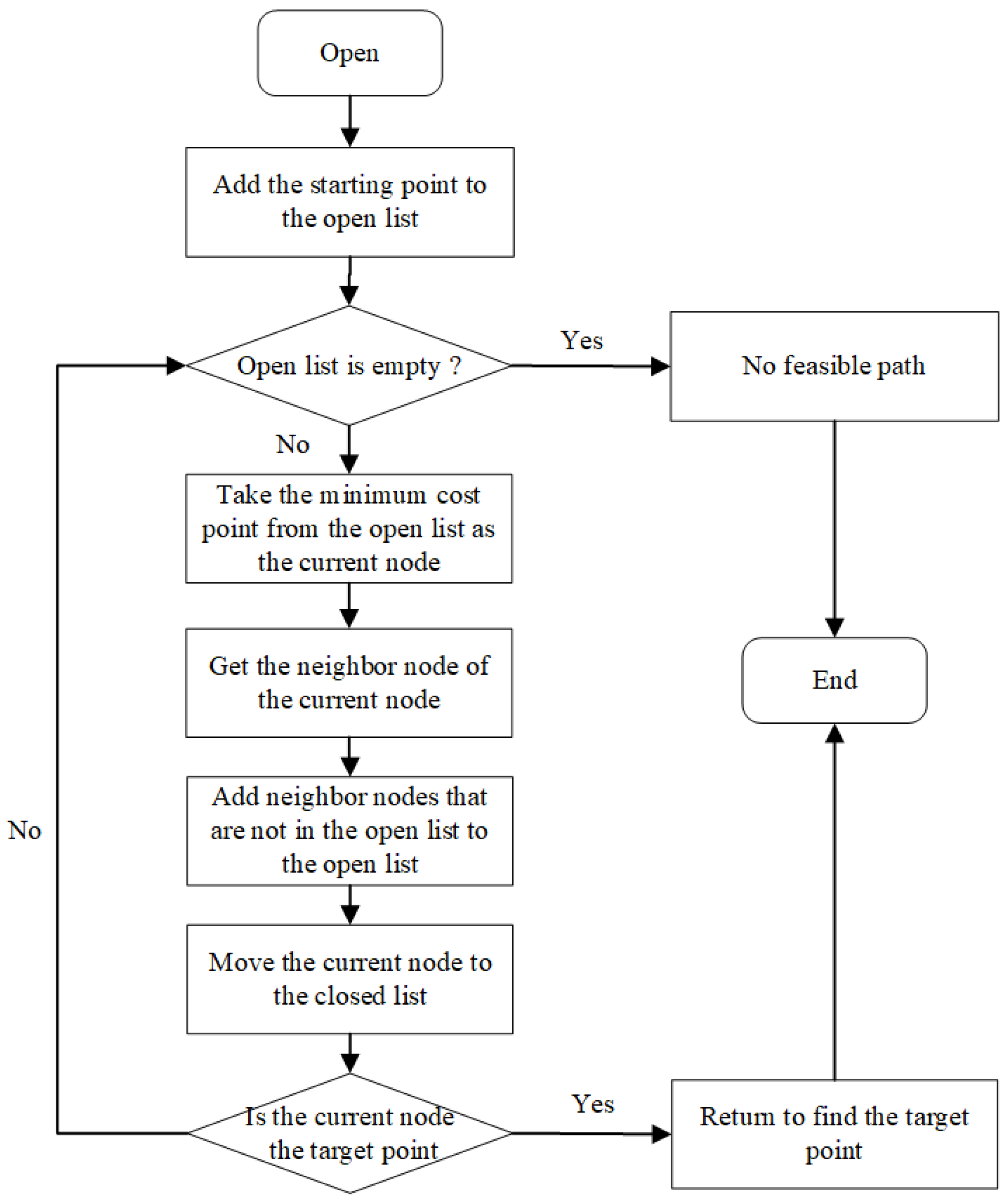
The search flow chart of the A* algorithm is shown in Figure 1. First, create a list of paths to store the path from the starting point to the target point. During the search process, maintain an open list and a closed list to store the nodes to be extended and the extended nodes. Each time, the node with the smallest total cost in the open list is selected as the current node of the search and moved into the closed list. Then, determine whether there are obstacles in the current node. If there are no obstacles, update the open list and the closed list. And judge whether the current node is the target point, if so, the feasible path is searched out.

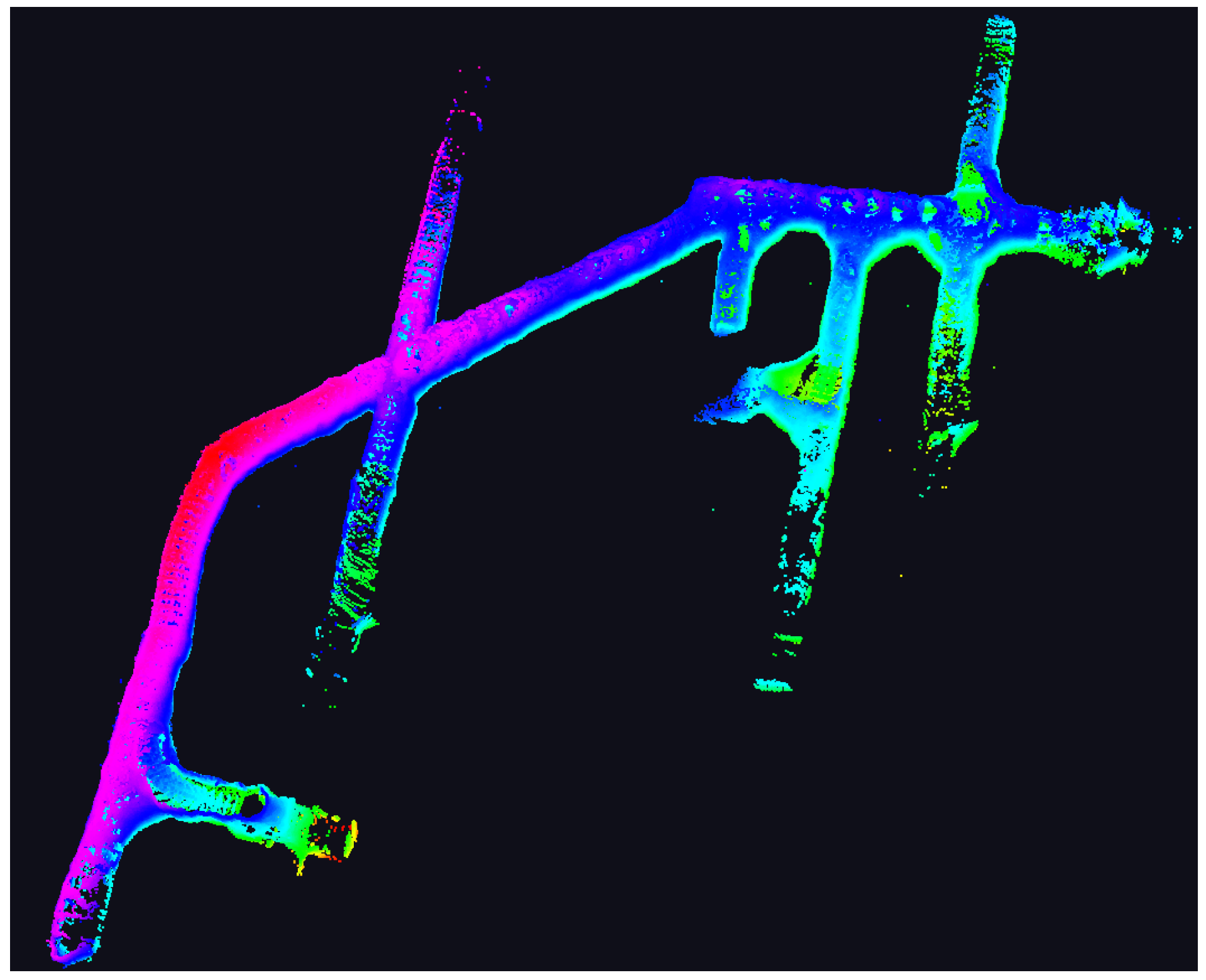
Global path planning is conducted based on a complete understanding of the environment. Accordingly, this paper acquired the three-dimensional point cloud data of an underground roadway at a working face of China Shanxi Zijin Mining Co., Ltd., as shown in Figure 2. The color map encodes point-cloud elevation, transitioning from red at the lowest points through orange, yellow, green, cyan, blue, to magenta at the highest points.

Due to the large volume of raw point cloud data and the difficulty of directly visualizing the internal structure of the roadway, the dataset was processed by filtering, down-sampling, and planarization, yielding the planarized point cloud map shown in Figure 3. As illustrated in Figure 3, the underground roadway map exhibits a complex and intricate structure, characterized by numerous branching passages and frequent turns. Additionally, the underground roadways are generally narrow, averaging around 4 m in width, which significantly increases the risk of collisions and poses considerable challenges to safe navigation. Subsequently, the processed point cloud was further converted into a grid map. Additional impassable obstacles were then introduced at the map boundaries and along interfaces with unexplored regions, ensuring complete closure of the underground roadway. This effectively prevents the planned paths from traversing unknown areas. 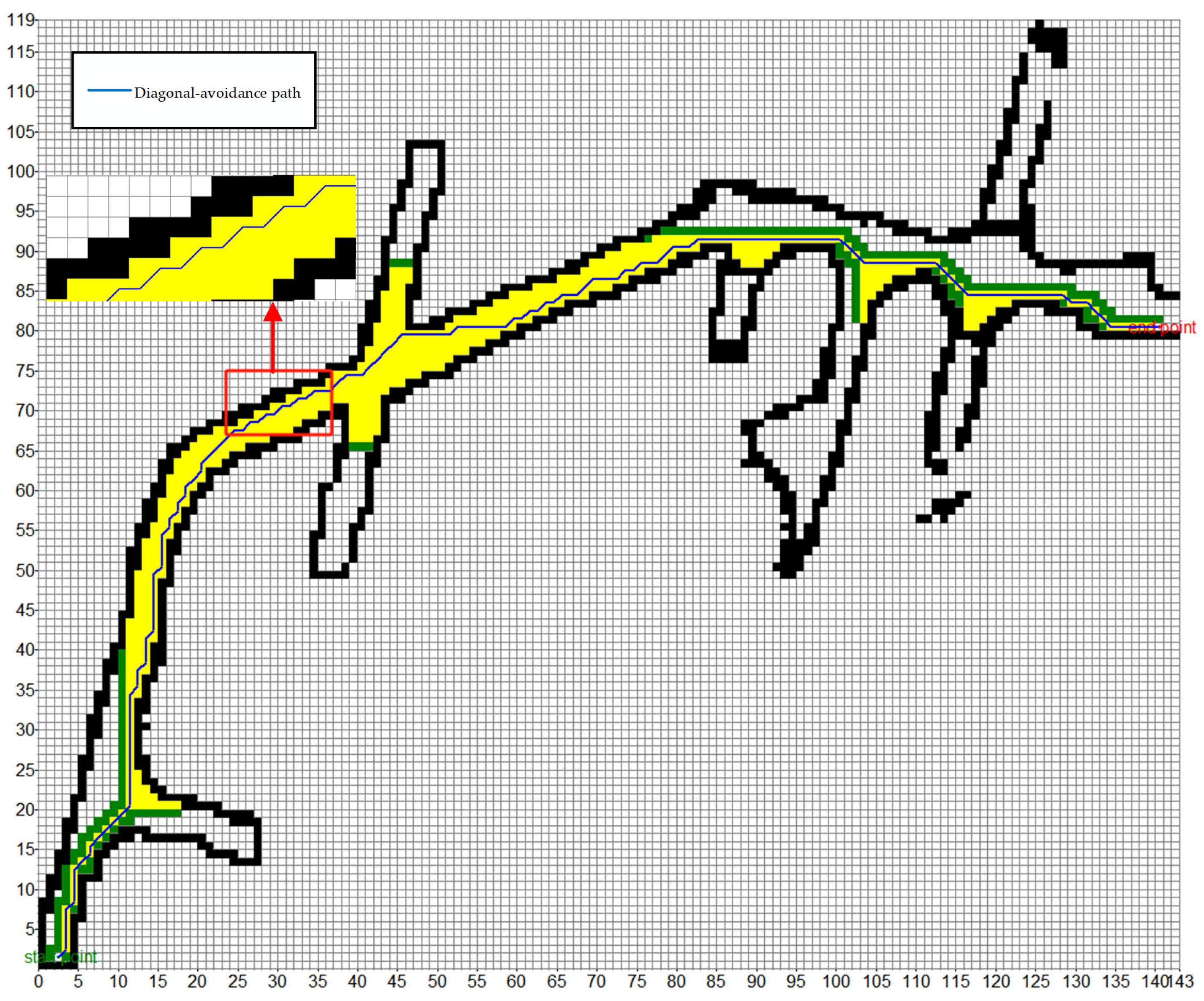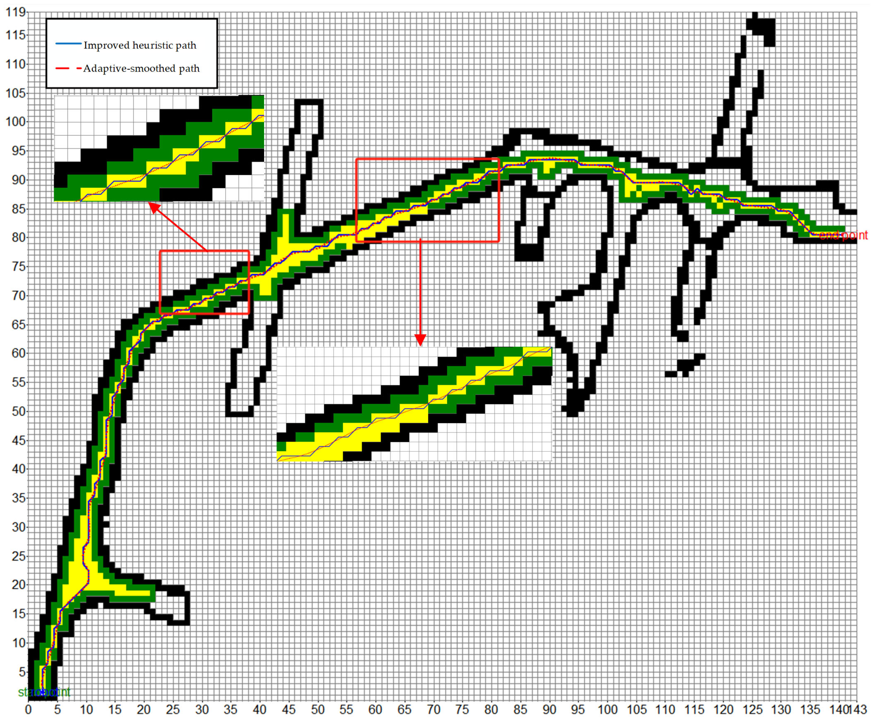Finally, the classic A* algorithm is employed for path planning, and the resulting path is shown in Figure 4.

The black grid in the figure is an obstacle, the mobile robot cannot walk, the blank area is a passable area, the yellow is marked as an extended node, and the green plus yellow is marked as a search node. It can be seen that the width of the roadway is different. The starting point and the end point can be randomly marked in the blank area of the figure.

It can be seen from the magnified view of Figure 4 that the classical A* algorithm has problems such as the path passing through the obstacle corner point, the path approaching the edge, and the inflection point not being smooth in the roadway grid map. This chapter improves the above three problems.

2.2. Anti-Diagonal Collision

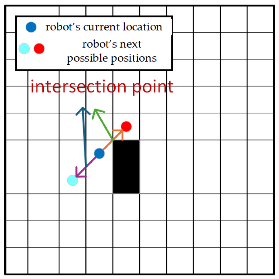
When the robot moves diagonally, it will directly cross the corner of the obstacle, which violates the safety requirements of the actual movement of the robot, which may lead to collision accidents. In order to solve this problem, the concept of the intersection point is introduced. The intersection point specifically refers to the key points that the robot must pass through when crossing the grid during oblique diagonal motion, as shown in Figure 5. The arrow points to an intersection.

In the execution of the path search algorithm, when facing the diagonal connection between the current node and the next node, the following steps need to be performed to determine whether the diagonal obstacle exists.

First, check the diagonal grid unit in another direction adjacent to the intersection. If either of the two grid units has an obstacle, it is determined that there is a diagonal obstacle.

If it is confirmed that there are diagonal obstacles, the current node should be removed from the Open List and added to the Closed List. Skip the node to avoid the path crossing the diagonal obstacle. If it is confirmed that there is no diagonal obstacle, the path search process is continued, the current node is obtained, and the forward or reverse search is performed according to the algorithm logic.

Taking Figure 5 as an example, if the blue node tries to move diagonally to the red node, the diagonal grid unit in the other direction adjacent to the intersection should be checked. If an obstacle is detected in the grid unit on the right side of the blue node, it is determined that the orange path is impassable and the path needs to be replanned. On the contrary, if the blue node moves to the light blue node, the inspection results show that the diagonal grid units in the other direction adjacent to the intersection have no obstacles, then the purple path can be determined as a passable path.

Through the above process, the path search algorithm can effectively judge the existence of diagonal obstacles when diagonally moving, and adjust the search strategy accordingly to ensure that the generated path does not cross obstacles and is a feasible path.

2.3. Improvement of Heuristic Function

The cost function of the classical A* search algorithm is shown in Formula (1).

$$f(n)=g(n)+h(n)$$

(1)

$f(n)$ is the total cost of the path of the node $n$, $g(n)$ is the actual cost from the starting point to the node $n$, and $h(n)$ is the heuristic function representing the estimated cost of the node $n$ to the target node.

The heuristic function usually selects the next extension point by calculating the distance from the current node to the target node. The design of the heuristic function has a great influence on search efficiency and path quality. The calculation method of the heuristic function usually has the following four calculation methods.

2.3.1. Euclidean Distance

The Euclidean distance is a linear distance between two points. The calculation is simple and intuitive. Its calculation formula is

$$h(n)=\sqrt{{(x_2-x_1)}^2+{(y_2-y_1)}^2}$$

(2)

2.3.2. Manhattan Distance

The Manhattan distance allows only horizontal and vertical movement. The calculation speed is faster and has a good performance on the grid map, but it may cause the path to be too long. Its calculation formula is

$$h(n)=\left|x_2-x_1\right|+\left|y_2-y_1\right|$$

(3)

2.3.3. Chebyshev Distance

The Chebyshev distance is the minimum distance between two points when diagonal movement is allowed. It is suitable for the grid environment that allows diagonal movement, especially the path search problem of diagonal movement in a grid map. Its calculation formula is

$$h(n)=\max (\left|x_2-x_1\right|,\left|y_2-y_1\right|)$$

(4)

2.3.4. Diagonal Distance

Diagonal distance is a heuristic function that combines Manhattan distance and Chebyshev distance. It considers the distance of moving in eight directions. It is suitable for the path search problem that allows horizontal, vertical, and diagonal movement in the grid. The calculation formula is

$$h(n)=\max (\left|x_2-x_1\right|,\left|y_2-y_1\right|)+(\sqrt{2}-2)\times \min (\left|x_2-x_1\right|,\left|y_2-y_1\right|)$$

(5)

The heuristic function of the A* algorithm is adjusted to the four different heuristic functions mentioned above, and tested in the roadway grid map environment shown in Figure 4. The comparison of the results is shown in

Table 1. Parameters comparison.

	Calculation Time	Search Nodes	Expanded Nodes	Number of Inflection Points
Euclidean distance	0.025	1036	999	88
Manhattan distance	0.0215	741	580	57
Chebyshev distance	0.023	1051	1018	74
Diagonal distance	0.0455	4520	4215	66

.

It can be seen from the data in the table that when the Manhattan distance is selected as the heuristic function, the calculation time is the shortest, the search nodes and the extended nodes are the least, and the number of inflection points is the least. Therefore, the Manhattan distance is selected as the heuristic function.

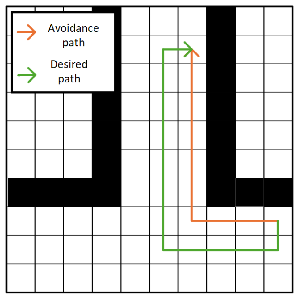
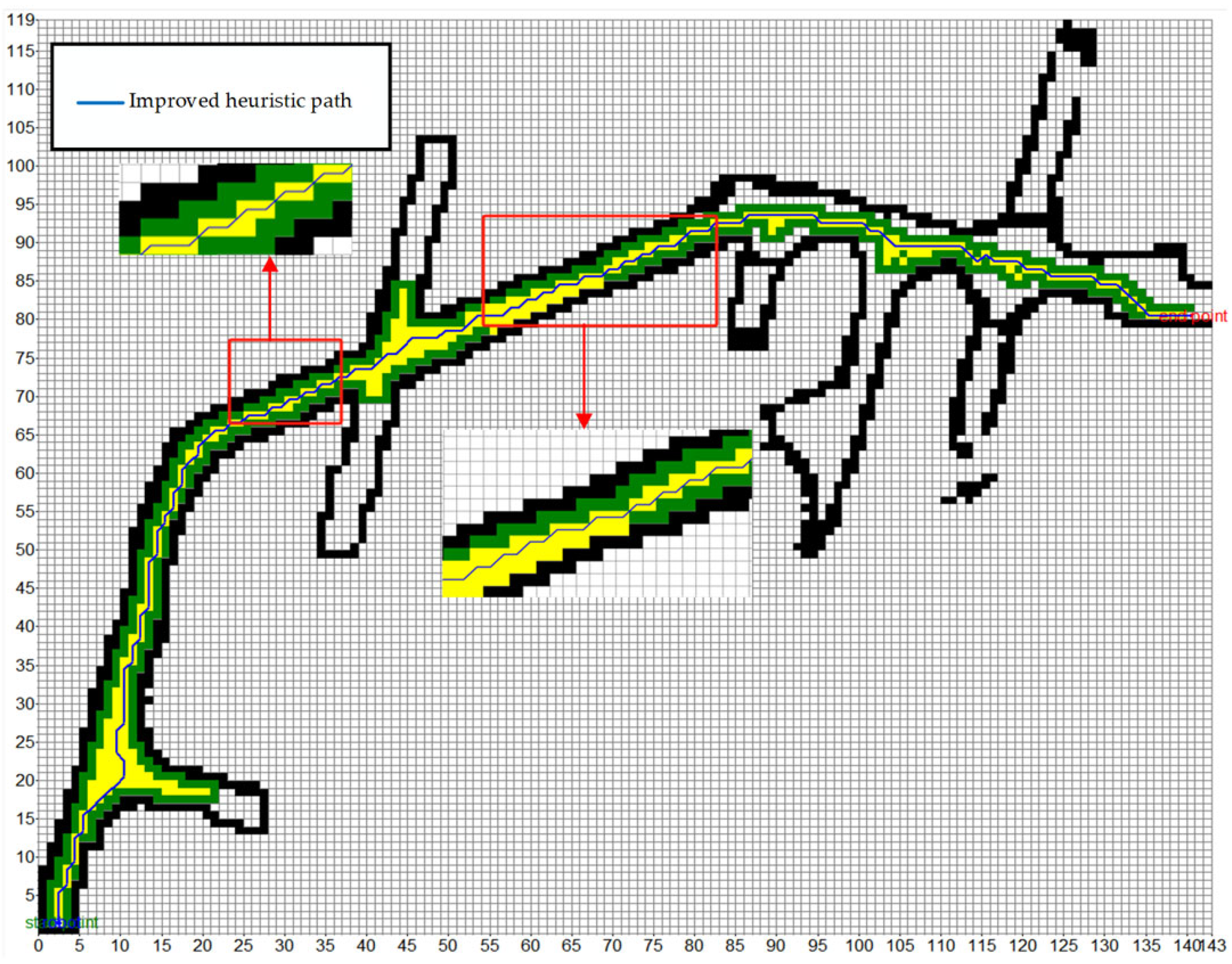
At the same time, considering the diversity of the width of the underground roadway, in order to ensure the safety of the path planning, the ideal path should be set in the central area of the roadway. However, the traditional heuristic function often tends to the edge of the roadway when planning the path, which undoubtedly increases the potential collision risk. Therefore, it is expected that the path planning algorithm can be more inclined to the area with a larger roadway width or the center of the roadway when selecting the path, so as to effectively reduce the possibility of collisions and improve the overall safety and reliability of the path. We expect that by optimizing the heuristic function, the performance of the A* algorithm in roadway path planning can be significantly improved. The expected effect is shown in Figure 6.

As shown in the diagram, the orange route represents the planned path diagram after anti-collision processing using the original Manhattan distance heuristic function. Obviously, the path tends to be close to the edge of the roadway. In contrast, the effect we expect to achieve is shown in the green route in the figure. The route is kept in the center of the roadway to ensure that the global path is basically always located in the middle of the roadway during the travel process.

Therefore, in order to achieve the desired path planning effect, the roadway width is integrated into the heuristic function as a key factor. The premise of this scheme is that the width information of the roadway where the current node is located can be accurately obtained from the grid map. The process of calculating roadway width information is shown in Figure 7.

If the channel width remembered is $d$, then the improved heuristic function is

$$h=h_{\mathrm{distance}}\times (1+\beta \times {\displaystyle \frac{1}{d+1}})$$

(6)

$h_{\mathrm{distance}}$ is the Euclidean distance and $\beta$ is the weight coefficient. The larger $\beta$ will increase the proportion of the roadway width in the heuristic function, which makes the path search algorithm more inclined to select those areas with more spacious space to avoid falling into narrow or limited space. The smaller $\beta$ will strengthen the dominant position of Euclidean distance in heuristic evaluation, which is equivalent to relaxing the constraint condition of roadway width on path selection, so that the algorithm pays more attention to the relative distance of the target position in the search process, and gives less consideration to the spaciousness of the surrounding environment.

The latter part is the penalty factor. If $d$ is very small, the penalty term becomes larger, which means that the path is very poor. The algorithm will increase the heuristic function value of this region, thereby reducing the possibility of selecting a narrow region. If $d$ is large, the penalty term is reduced, indicating that the path is more spacious and the traffic is good, the algorithm will give priority to these areas.

2.4. Adaptive B-Spline Curve Smoothing

It can be seen from Figure 4 that the global path planned by the classical A* algorithm is not smooth, and there are many spikes at the inflection point, which may lead to sharp turns and poor dynamic environment adaptability, which is not conducive to the actual movement of mobile robots. Therefore, a smoothing algorithm is needed to smooth the global path. Both B-spline curves and Bezier curves can be used to smooth curves. However, Bezier curve has poor local control ability when dealing with curve smoothing, and it is difficult to express complex routes efficiently through a Bezier curve. Therefore, the B-spline curve is selected to smooth the global path to generate a continuous and smooth road, thereby improving the driving performance of the robot.

Set $n+1$ control points $P_0$, $P_1$, $P_2$, …. These control points are used to define the direction and boundary range of the spline curve. The definition of the $k$-order B-spline curve with $n$ control points is

$$P(u)=\left[P_0 P_1 \dots P_{\mathrm{n}}\right]\left[\begin{array}{c}{B}_{0,k}(u)\\ B_{1,k}(u)\\ \dots \\ B_{n,k}(u)\end{array}\right]{\displaystyle \sum _{i=0}^n{B}_{i,k}(u)P_i}$$

(7)

In the formula, $B_{i,k}(u)$ is the $i-th$ $k$-order B-spline basis function, corresponding to the control point $P_i$. $u$ is the independent variable.

The two key indicators of B-spline curves are order $k$ and smoothing factor $k$. $k$ defines the degree of polynomial segments. The larger $k$ is, the smoother the curve is, but the key turning points and details in the path may be lost. Lower $k$ may lead to more inflection points in the curve. The larger $s$ makes the curve smoother but may deviate from the original control point, and the smaller $s$ closely fits the original path, but it is difficult to effectively eliminate noise and small fluctuations. Therefore, how to choose the values of $k$ and $s$ is very important for the smoothing effect of B-spline curves.

At the same time, if fixed $k$ and $s$ are used, then there will be obvious limitations in the diversification path. The path may be too smooth when the path is simple, resulting in deviation and loss of key features; when the path is complex, the smoothness is insufficient, and the turning and fluctuation cannot be effectively eliminated, which affects the coherence and execution efficiency of the path. Therefore, it is necessary to design an adaptive B-spline curve smoothing strategy to dynamically adjust the parameters according to the complexity and characteristics of the path, so that the path can achieve the best smoothing effect in different scenarios. When the path complexity is high, higher parameters are selected to generate smoother and more coherent curves and reduce the turning frequency. When the path complexity is low, the lower parameters are selected to avoid the path deviation caused by excessive smoothing.

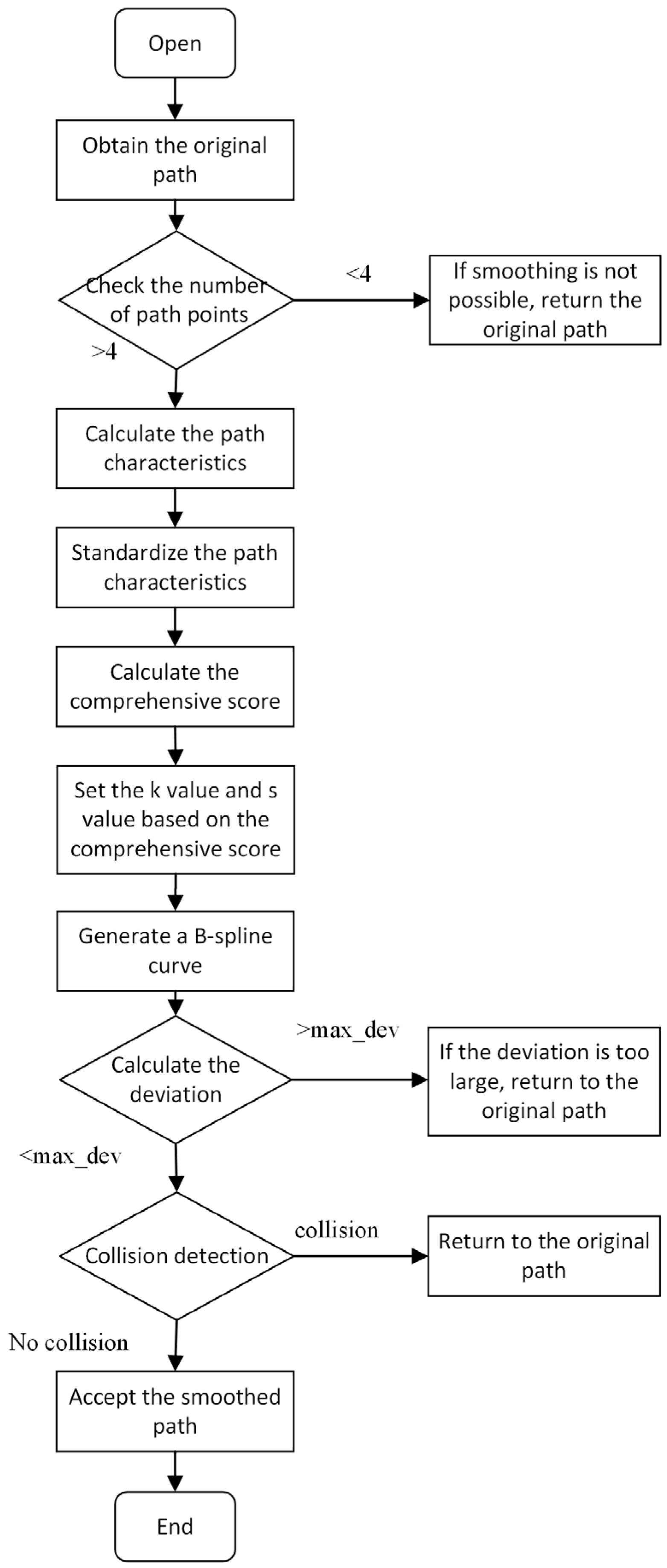
The flow chart of the adaptive B-spline curve smoothing method is shown in Figure 8.

This method first needs to verify whether the number of points in the original path is more than four, because the order of the B-spline curve is equal to the degree of the polynomial segment. For $n-order$ B-spline curves, at least $n+1$ control points are required. In view of the fact that the minimum 3-order B-spline curve is used in the adaptive smoothing method, and the 3-order B-spline curve requires at least four control points, it is necessary to verify whether the number of original path points is greater than four. Then, four key features are extracted from the original path (path length, mean curvature, fluctuation degree, and direction change rate), and these eigenvalues are normalized to the interval of 0 to 1. The normalized values of the four path features are $L_{norm}$ (path length), $C_{norm}$ (mean curvature), $F_{norm}$ (fluctuation degree), and $R_{norm}$ (direction change rate), respectively. The corresponding weights are $w_L,w_C,w_F,w_R$, and the sum of their weights is one.

The comprehensive score is

$$score=w_L \cdot L_{norm} +w_C \cdot C_{norm} +w_F \cdot F_{norm }+w_R \cdot R_{norm}$$

(8)

Select the $k$ value according to the range of $score$.

$$k=\left\{\begin{array}{l}3 \mathrm{if} \mathrm{score}<0.25\\ 4 \mathrm{if} 0.25\le \mathrm{score}<0.5\\ 5 \mathrm{if} 0.5\le \mathrm{score} \text{<}0.75\\ 6 \mathrm{if} \mathrm{score} \ge 0.75\end{array}\right.$$

(9)

The smoothing factor is calculated by the following formula

$$s=score\times {\left(\max \_deviation\right)}^2$$

(10)

After determining the order and smoothing factor of the B-spline curve, the corresponding degree of the spline curves can be selected to smooth the global route. However, it is necessary to evaluate whether the smoothed path exceeds the preset maximum deviation limit, which is designed to control the degree of deviation of the smoothed path from the original path, thereby ensuring the accuracy and feasibility of the path. The maximum deviation is defined as the maximum distance from the point on the smooth path to the nearest point on the original path. The specific deviation calculation formula is

$$D=\underset{p^{\prime }\in smooth path}{\max }\left(\underset{p\in original path}{\min }‖p^{\prime }-p‖\right)$$

(11)

$p^{\prime }$ is the point on the smooth path. $p$ is the point on the original path. $‖p^{\prime }-p‖$ denotes the Euclidean distance between two points.

Finally, it is necessary to verify whether the smoothed path collides with the obstacle. If a collision occurs, the system will resume using the original path; if no collision occurs, the smoothed path is accepted and adopted.

3. Fusion of Improved A* and DWA Algorithm

Although the improved A* algorithm can avoid known obstacles, the following situations may occur during the movement of the handling robot, such as large pieces of ore falling in the roadway, miners, and equipment moving. This requires the handling robot to achieve dynamic obstacle avoidance. The tracked chassis is a differential drive model, and the DWA algorithm is commonly used as a local path planning algorithm to achieve the function of dynamic obstacle avoidance. However, the DWA algorithm falls easily into a local optimum if there is no global path information. Therefore, the global path planning and local path planning are combined to achieve the purpose of dynamic obstacle avoidance.

3.1. Moving Trajectory Model of Handling Robot

DWA is a local path planning method based on the current state and dynamic window of the robot. Its core goal is to quickly generate an optimal trajectory in a short period of time based on the current position, speed, and environmental information of the robot. These trajectories are achieved by selecting the linear velocity and angular velocity suitable for the current state and environment.

$$\left\{\begin{array}{l}{x}_{n+1}=x_n+v\Delta t\cos {\theta }_{n-1}\\ y_{n+1}=x_n+v\Delta t\sin {\theta }_{n-1}\\ {\theta }_{n+1}=x_n+\omega \Delta t\end{array}\right.$$

(12)

$x_{n+1}$, $y_{n+1}$, and ${\theta }_{n+1}$ are the position information of the handling robot at the next moment; $x_n$, $y_n$, and ${\theta }_n$ are the position information of the handling robot at the current moment; $v$ and $\omega$ are the linear velocity and angular velocity of the handling robot, and $\Delta t$ is the sampling time.

3.2. Sampling Speed

Due to the hardware design, architecture composition, and environmental conditions of the handling robot, the speed sampling space of the handling robot is limited. Mainly divided into three categories.

3.2.1. Velocity Boundary Limitation

According to the hardware design of the handling robot and the limitations of the underground environment, there is a boundary limit on its speed. At this time, the sampling speed space $V_m$ is

$$V_m=\left\{(v,w)|v\in \left[v_{\min },v_{\max }\right],\omega \in \left[{\omega }_{\min },{\omega }_{\max }\right]\right\}$$

(13)

$v_{\min },v_{\max }$ are the minimum linear velocity and the maximum linear velocity of the handling robot. ${\omega }_{\min },{\omega }_{\max }$ are the minimum angular velocity and the maximum angular velocities of the handling robot.

3.2.2. Acceleration Limitation

Due to the limitations of the driving motor of the handling robot, the linear acceleration and angular acceleration also have boundary restrictions. Assuming that the maximum acceleration is equal to the maximum deceleration, the sampling speed space $V_d$ is

$$V_d=\left\{\left(v,\omega \right)\left|\begin{array}{l}v\in \left[v_c-a_{v\max }\cdot \Delta t,v_c+a_{v\max }\cdot \Delta t\right]\\ \omega \in \left[{\omega }_c-a_{\omega \max }\cdot \Delta t,{\omega }_c+a_{\omega \max }\cdot \Delta t\right]\end{array}\right.\right\}$$

(14)

$v_c$ and ${\omega }_c$ are the current linear velocity and angular velocity of the handling robot. $a_{v\max }$ and $a_{\omega \max }$ are the maximum linear acceleration and maximum angular acceleration of the handling robot.

3.2.3. Environmental Obstacle Limitation

Because of the need to consider real-time obstacle avoidance, the obstacles around the handling robot should be considered. The constraint condition that it does not collide with the surrounding obstacles is

$$V_a=\left\{\left(v,\omega \right)\left|\begin{array}{l}v\in \left[v_{\min },\sqrt{2\cdot dist(v,\omega )\cdot a_{v\max }}\right]\\ \omega \in \left[{\omega }_{\min },\sqrt{2\cdot dist(v,\omega )\cdot a_{\omega \max }}\right]\end{array}\right.\right\}$$

(15)

$dist(v,\omega )$ represents the nearest distance between the simulated trajectory and the obstacle at the current speed. In the absence of obstacles, $dist(v,\omega )$ is a large constant. When the sampling speed of the robot is within its range, it can achieve safe deceleration with the constraint of maximum deceleration until it avoids obstacles.

The speed combination $v_r$ that the final handling robot can take needs to meet the intersection of the following three constraints.

$$V_r=v_m\cap v_d\cap v_a$$

(16)

After the constraint is determined, the DWA algorithm samples in this space with a certain resolution. $E_v$ and $E_{\omega }$ are used to represent the sampling resolution of linear velocity and angular velocity, respectively, then $n$ sets of velocities will be taken in this sampling space.

$$n=\left[{\displaystyle \frac{v_{high}-v_{low}}{E_v}}\cdot {\displaystyle \frac{{\omega }_{high}-{\omega }_{low}}{E_{\omega }}}\right]$$

(17)

$v_{high}$, $v_{low}$, ${\omega }_{high}$, and ${\omega }_{low}$ are the upper and lower limits of the velocity space.

When the Dynamic Window Approach (DWA) samples a series of candidate linear velocities $v$ and angular velocities $\omega$ within the dynamic window, the system sequentially invokes the kinematic model of the differential-drive chassis to ‘predict’ each velocity pair over a short time horizon. First, the model enforces the robot’s physical limits by clipping sampled velocities according to its maximum and minimum linear speeds and maximum linear/angular accelerations, ensuring all candidates lie within the chassis’ actual performance envelope. Next, using the robot’s circumscribed circle as a safety boundary, each predicted trajectory undergoes collision checking, and any trajectory that may intersect with environmental obstacles is automatically discarded. Finally, the remaining feasible trajectories are mapped directly to executable drive–command velocities. Through this process, the kinematic model acts both as a physical-constraint filter—guaranteeing that velocity samples do not exceed hardware limits—and as a safety validator—preserving only collision-free paths—ultimately yielding a set of safe, reliable, and truly executable motion plans.

3.3. Optimizing Evaluation Function

Once a set of feasible trajectories is obtained, each trajectory is evaluated to identify the optimal one, and its corresponding velocity is selected as the driving speed. The DWA evaluation function before optimization is

$$G(v,\omega )=\alpha \cdot T(v,\omega )+\beta \cdot V(v,w)+\gamma \cdot D(v,\omega )$$

(18)

where $T(v,\omega )$ is the objective cost function, $V(v,w)$ is the speed cost function, $D(v,\omega )$ is the obstacle cost function $\alpha$, $\beta$, and $\gamma$ are the weighting coefficients. $T(v,\omega )$ represents the distance deviation between the end of the trajectory and the target point in the current group. The larger the deviation is, the larger the value $V(v,w)$ is

$$V(v,w)=v_{max} -v_{end}$$

(19)

Among them, $v_{max}$ is the set maximum linear speed, and $v_{end}$ is the current terminal speed. The smaller the terminal speed, the greater the value; that is, it is hoped to ensure high speed under the premise of ensuring safety.

$$D(v,\omega )={\displaystyle \frac{1}{min\_dist\_to\_obstacle }}$$

(20)

$min\_dist\_to\_obstacle$ is the minimum distance between the trajectory and the nearest obstacle; the smaller the distance, the greater the value to achieve the purpose of preventing collision.

The traditional DWA evaluation function easily makes the handling robot fall into the local optimal over-obstacle avoidance when avoiding obstacles, resulting in a wide range of detours or falling into a dead end in the case of complex paths. Therefore, a deviation cost function is added to the evaluation function. The modified evaluation function is

$$G(v,\omega )=\alpha \cdot T(v,\omega )+\beta \cdot V(v,w)+\gamma \cdot D(v,\omega )+F(v,\omega )$$

(21)

$F(v,\omega )$ is the deviation distance evaluation function, specifically

$$F(v,\omega )=\left\{\begin{array}{l}0 if avg\_dev\le d_{\max }\\ \lambda \times (avg\_dev-d_{\max }) avg\_dev>d_{\max } \end{array}\right.$$

(22)

where $\lambda$ is the weight coefficient, $d_{\max }$ is the maximum allowable deviation $avg\_dev$ represents the average deviation of the trajectory from the global path. The calculation method is as follows:

• For each trajectory generated by DWA, the Euclidean distance from each point on the trajectory to the nearest point in the global path is calculated.
• The minimum distance of all points is accumulated, then divided by the number of points on the trajectory, and the average deviation is obtained.

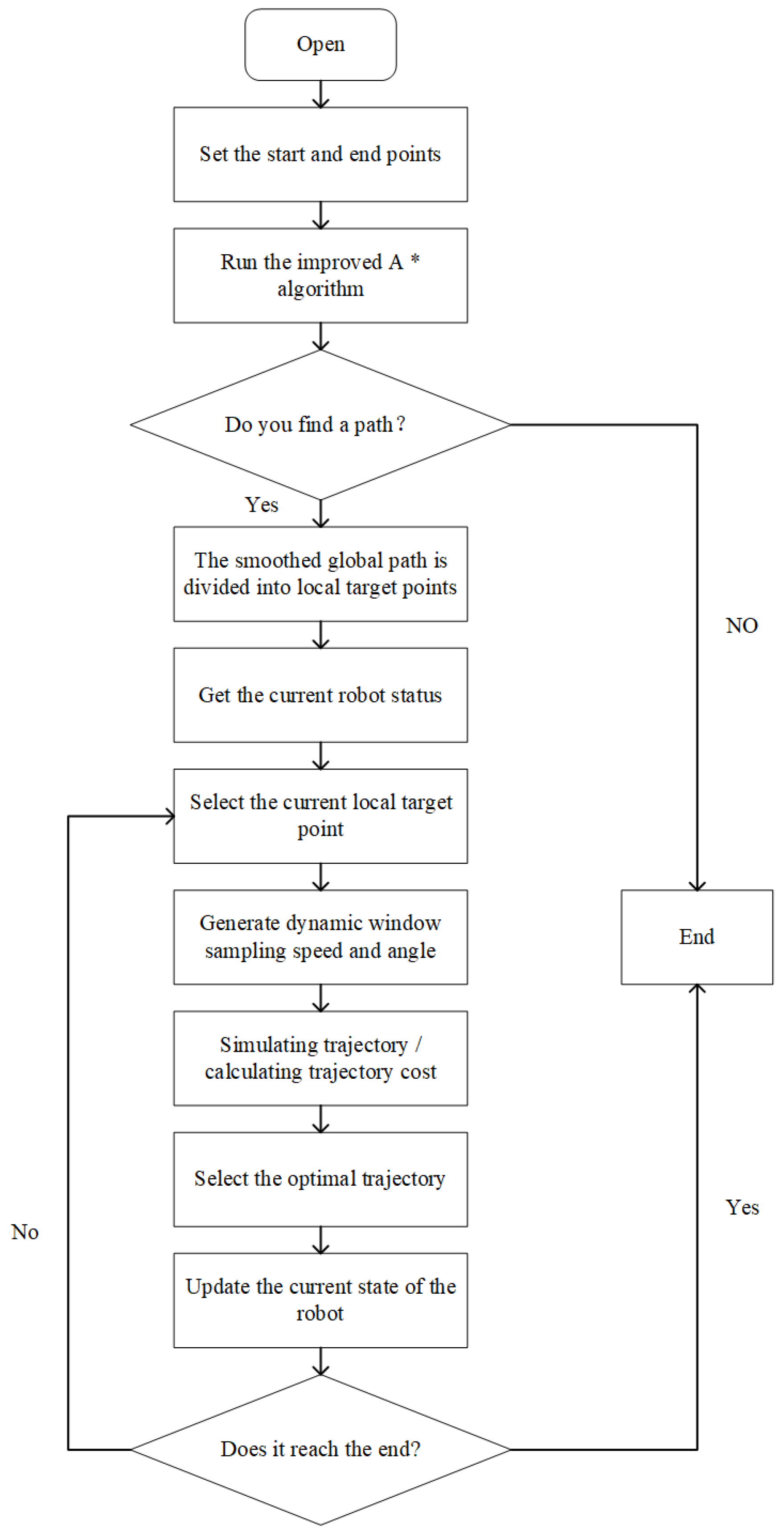
3.4. Fusion of Improved A* and Improved DWA Algorithm

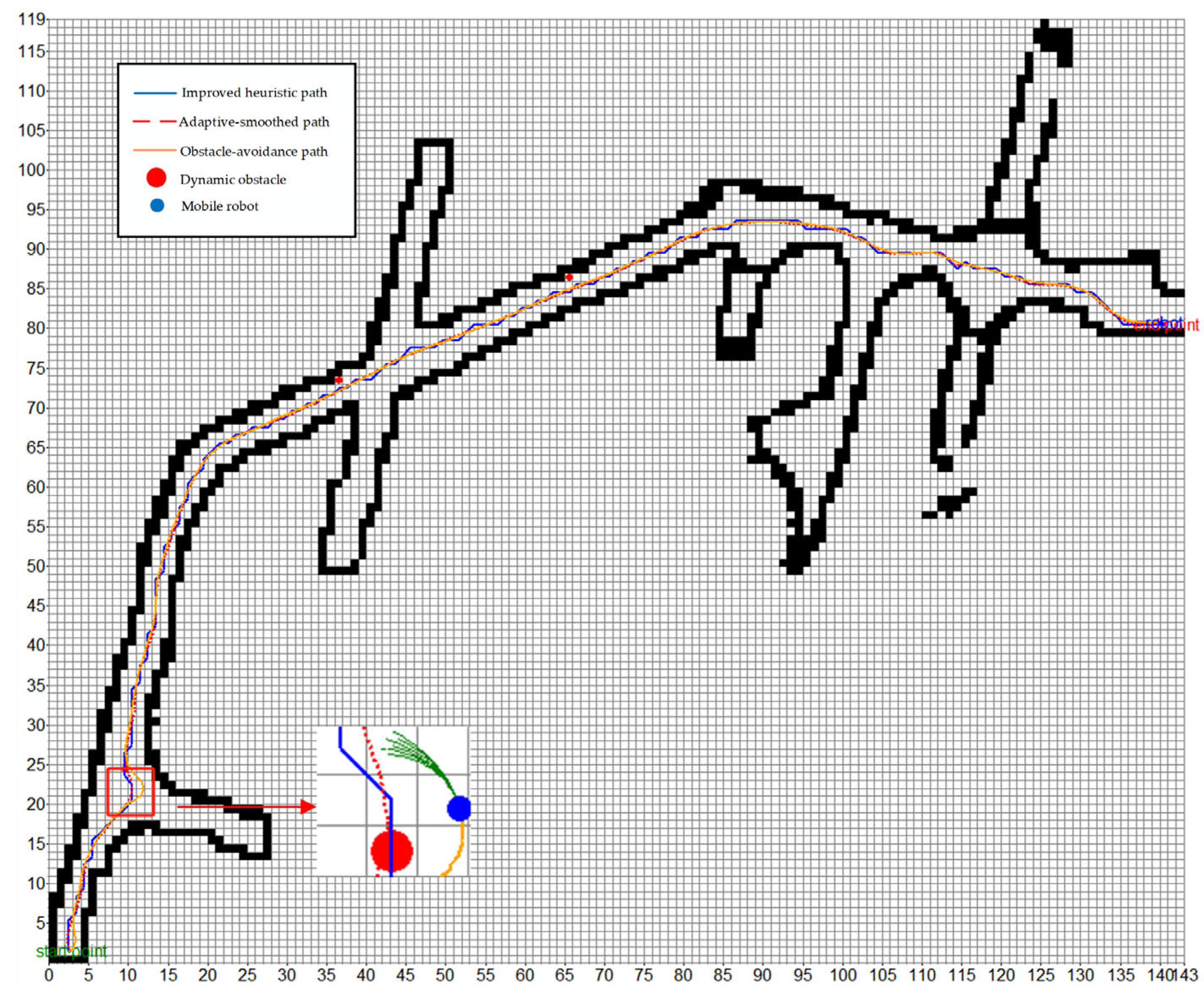
This paper combines the improved A* algorithm with the improved DWA algorithm. The adaptive A* algorithm is used to obtain the smoothed global path, which is divided into multiple local target points. In the control cycle, the DWA uses the improved evaluation function to select the best trajectory according to the current local target point, the current state of the robot, and the environment. Once close to the current local target point. DWA will switch to the next target point until it reaches the end point. The specific process is shown in Figure 9.

4. Experiment and Analysis

4.1. Improved A* Algorithm Experiment

Based on the above algorithm design ideas, in order to verify the effectiveness and feasibility of the improved adaptive A* algorithm, the same starting point and end point are set in the grid map of Figure 4 for path planning experiments.

4.1.1. Anti-Diagonal Collision Experiment

In Section 2.2, it is elaborated in detail that the purpose of introducing the intersection point is to avoid the robot directly crossing the corner point of the obstacle when moving diagonally. The relevant experiment results are shown in Figure 10.

By comparing Figure 10 and Figure 4, it can be clearly observed that direct contact with the obstacle corner is successfully avoided after the concept of the intersection point is introduced. The comparison results fully verify the effectiveness and practicability of the proposed anti-diagonal collision strategy.

4.1.2. Improved Heuristic Function Experiment

In Section 2.3, in order to make the path planning choose the path in the middle of the roadway or give priority to the width of the roadway, the consideration of roadway width is introduced into the heuristic function, and the experiment results are shown in Figure 11.

Comparing Figure 10 and Figure 11, it can be observed that the A* algorithm optimized by the heuristic function will produce some unnecessary inflection points in the path planning, but it is obvious that it tends to choose the path in the center of the roadway. This change effectively solves the problem that the mobile robot may touch the edge of the roadway in actual movement. The redundant inflection points in the path can be effectively improved by the adaptive curve smoothing method introduced in the subsequent chapters.

4.1.3. Adaptive Curve Smoothing Experiment

In Section 2.4, a method of adaptively selecting the order and smoothing factor of B-spline curve smoothing according to the characteristics of the global path planning route is introduced. After many experiments, the maximum offset is set to 3.0, and the weights are respectively $w_L=0.1$, $w_C=0.4$, $w_F=0.4$, and $w_R=0.1$. Adaptive selection of $k$ is 3, and $s$ is 10.91. The experiment results are shown in Figure 12.

In the figure, the blue line represents the original unsmoothed path, while the red line shows the path after adaptive B-spline smoothing. It can be seen from the figure that the smoothed path shows the characteristics of smooth and non-obtrusive inflection points, effectively reducing the number of inflection points increased by the heuristic function adjustment, and successfully crossing unnecessary continuous inflection points. On the whole, the smoothed path basically fits the original path, while ensuring no contact with obstacles.

In view of the above three improvement measures, the specific evaluation indicators after the gradual implementation of each stage are summarized in the following

Table 2. Comparison table after improvement of each step.

	Calculation Time	Search Nodes	Extended Nodes	Number of Inflection Points
Original A*	0.0215	741	580	57
A* with Diagonal Collision	0.04	735	568	67
A* with Modified Heuristic Function	0.03	817	326	56
A* after Adaptive B-Spline Curve Smoothing	0.018	817	326	11

.

According to the data in Table 2, it can be seen that the improved A* algorithm shows a series of significant advantages after introducing the diagonal anti-collision detection mechanism, integrating the roadway width into the heuristic function, and adopting the adaptive B-spline curve smoothing method. Specifically, the number of extended nodes decreased by 43.79%, the calculation time decreased by 16.28%, and the number of inflection points decreased by 80.70%. The intuitive display of Figure 12 and the detailed data of Table 2 verify the effectiveness and superiority of the proposed improved algorithm.

4.2. Fusion of Improved A* and DWA Algorithm Experiment

In this system, the panel settings for maximum/minimum linear velocity, maximum angular velocity, and maximum linear acceleration directly determine the velocity bounds available to DWA at each frame, ensuring that the algorithm never issues commands beyond the differential-drive platform’s capabilities. The linear velocity resolution, angular velocity resolution, and time step together control the discretization of the velocity interval and the fidelity of short-term trajectory simulation. The three cost weights—goal cost weight, obstacle cost weight, and deviation cost weight—adjust the priority of moving toward the subgoal, maintaining clearance from obstacles, and adhering to the global path when evaluating feasible trajectories. Thus, the GUI parameters are tightly coupled with the kinematic model of the differential-drive robot and the trajectory evaluation. Specifically, in Chapter 3, we set these parameters as follows: maximum linear velocity 1 m/s; minimum linear velocity 0 m/s; maximum angular velocity 1 rad/s; maximum linear acceleration 0.2 m/s²; linear velocity resolution 0.1 m/s; angular velocity resolution 0.1 rad/s; time step 0.1 s; goal cost weight 3.0; obstacle cost weight 5.0; and deviation cost weight 3.0. This configuration enables the robot to perform local planning efficiently and safely in complex environments, ensuring both consistent global-path tracking and robust dynamic obstacle avoidance.

4.2.1. Static Obstacle Avoidance Experiment

Firstly, the obstacle avoidance experiment of static obstacles is carried out, and the results are shown in Figure 13. In the figure, the blue solid line represents the globally planned path, the red dashed line, its smoothed counterpart, and the orange solid line, the DWA-based obstacle-avoidance trajectory. Labels ①, ②, and ③ denote the sequential avoidance maneuvers for static obstacles introduced after the global planning phase. As shown in the figure, the fused algorithm can safely and collision-freely avoid the new static obstacles, and basically travel along the smoothed global path outside the obstacle avoidance part. In the process of obstacle avoidance, the algorithm will not deviate significantly from the original path, nor will it fall into the local optimum, which will lead to the situation that the original path cannot be found by avoiding the obstacle around the big bend, whereby the expected effect is achieved.

4.2.2. Dynamic Obstacle Avoidance Experiment

Secondly, the dynamic obstacle avoidance experiment is carried out. The dynamic obstacle (red circle) is added to the map. The result of the selection algorithm is shown in Figure 14. The red box selection part in the figure is the obstacle avoidance process. It can be seen that the algorithm is as expected. When encountering dynamic obstacles, it begins to plan an expected trajectory to avoid dynamic obstacles.

4.3. Applicability Verification

To validate the applicability of the improved fusion algorithm in environments beyond the fixed grid map used in the previous experiment, This paper also selects the underground roadway scene of a working face of Anhui Development Mining Co., Ltd. (Lu’An, China) as an example. and applied the enhanced algorithm to perform global path planning as well as static and dynamic obstacle-avoidance experiments. The resulting experiment outcomes are presented in Figure 15, Figure 16 and Figure 17.

As illustrated in Figure 15, the refined A* algorithm generates a global trajectory that remains closely aligned with the underground roadway centerline. The path exhibits gentle curvature variations, a substantially lower waypoint (turning-point) count, and no abrupt angular discontinuities.

Figure 16 substantiates the robustness of the integrated planning framework when confronted with newly introduced static obstacles. Although the global route is pre-computed, the mobile platform autonomously perceives emergent impediments and, at the three representative loci (①–③), performs on-the-fly local replanning to negotiate collision-free detours.

The dynamic obstacle experiment depicted in Figure 17 further underscores the system’s adaptability. Upon detecting that an obstacle ahead possesses a forward motion trend, the planner extrapolates its future states via a trajectory-prediction module and subsequently invokes the Dynamic Window Approach (DWA) to synthesize a rapid circumvention maneuver, thereby mitigating collision risk while preserving progress toward the goal.

Collectively, these three evaluations demonstrate that the proposed Refined A* algorithm and the Refined A* + DWA hybrid planner are not restricted to a single, idealized grid environment; rather, they exhibit strong generalizability and scenario adaptability across a diverse, real-world underground roadway map.

5. Conclusions

Because the classical A* algorithm has some limitations in the field of path planning, especially in dealing with the problems of obstacle corner collision, unsmooth path, and sharp turning point when the diagonal moves, it is difficult to adapt to the motion characteristics of the actual mobile robot. In the specific application scenario of underground roadway planning, the path planned by the algorithm is often close to the edge of the roadway, which increases the potential collision risk.

Therefore, in view of the above problems, this paper proposes an optimized adaptive A* algorithm. Firstly, the algorithm defines the concept of the intersection point. By checking the state of two adjacent grids on the other side of the intersection point, the collision problem when the diagonal line moves is effectively avoided. Secondly, the factor of roadway width is integrated into the heuristic function, which makes the path planning algorithm more inclined to the middle area of the roadway when selecting the path, thus reducing the collision risk. At the same time, the adaptive B-spline curve is used to dynamically adjust the order and smoothing factor according to the complexity of the global path, and the path is smoothed.

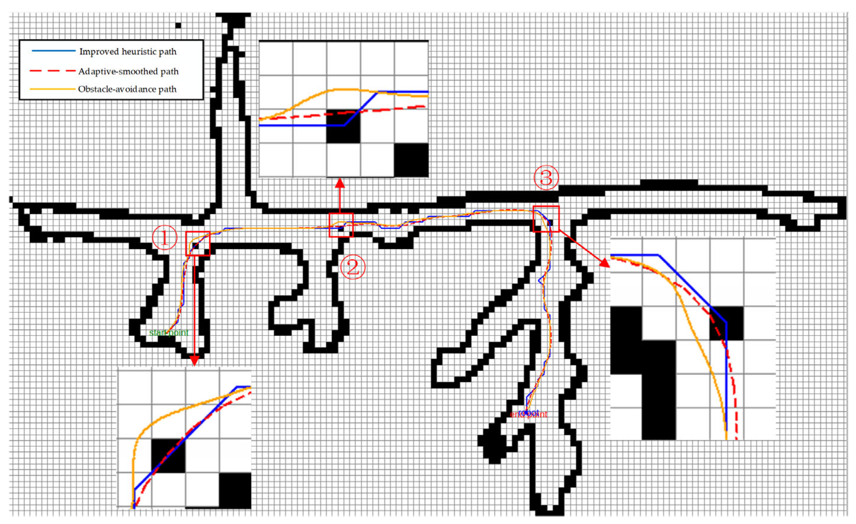
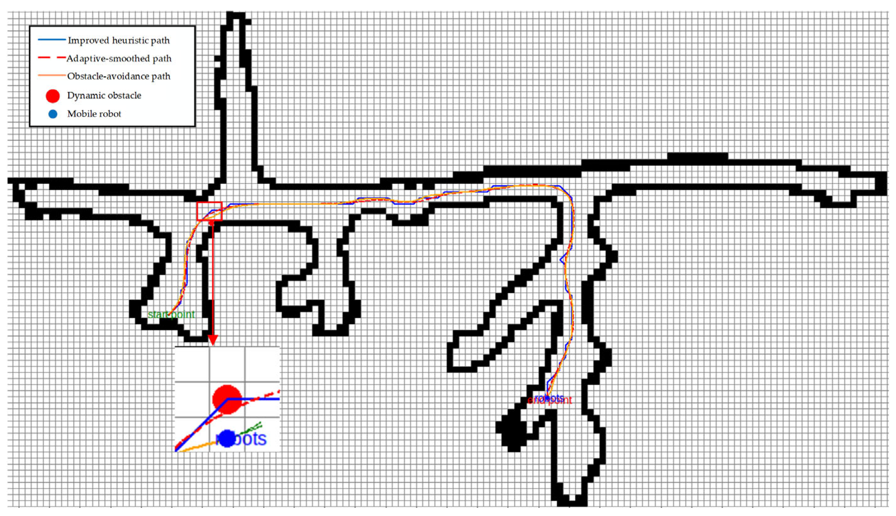
Then, the improved A* algorithm is combined with the improved DWA algorithm to achieve dynamic obstacle avoidance. Finally, the experiment proves that the path planned by the optimized A* algorithm is not only closer to the center of the roadway, but also the path is smooth, and the number of inflection points is greatly reduced. Compared with the original algorithm, the optimization algorithm can avoid collisions with the obstacle corner when the diagonal moves, which is more in line with the actual motion requirements of the mobile robot. At the same time, the fused path planning algorithm can avoid the new static obstacles and dynamic obstacles, and meet the requirements of dynamic obstacle avoidance. In addition, we conducted supplementary experiments on the new Ankai underground roadway map to further verify the effectiveness and applicability of the proposed algorithm in complex underground roadway environments.