Machine Learning Ship Classifiers for Signals from Passive Sonars

Abstract

The accurate automatic classification of underwater acoustic signals from passive SoNaR is vital for naval operational readiness, enabling timely vessel identification and real-time maritime surveillance. This study evaluated seven supervised machine learning algorithms for ship identification using passive SoNaR recordings collected by the Brazilian Navy. The dataset encompassed 12 distinct ship classes and was processed in two ways—full-resolution and downsampled inputs—to assess the impacts of preprocessing on the model accuracy and computational efficiency. The classifiers included standard Support Vector Machines, K-Nearest Neighbors, Random Forests, Neural Networks and two less conventional approaches in this context: Linear Discriminant Analysis (LDA) and the XGBoost ensemble method. Experimental results indicate that data decimation significantly affects classification accuracy. LDA and XGBoost delivered the strongest performance overall, with XGBoost offering particularly robust accuracy and computational efficiency suitable for real-time naval applications. These findings highlight the promise of advanced machine learning techniques for complex multiclass ship classification tasks, enhancing acoustic signal intelligence for military maritime surveillance and contributing to improved naval situational awareness.

1. Introduction

There has been an increasing interest recently in research on maritime vessels. A submarine is an advanced instrument for maritime deterrence as a specialized platform for the surveillance of sudden attacks. The submarine remains hidden while scanning the environment to effectively perform its tasks. Then, it operates silently using acoustic and electromagnetic waves, avoiding any signal emission while passively listening to the environment. While previous studies have shown promising results in ship classification using synthetic or simplified SoNaR data [1,2], there is a lack of validation on real-world, multiclass datasets recorded under operational conditions. This gap limits the deployment of these models in practical naval surveillance scenarios. Therefore, this study explored machine learning for ship classification using underwater acoustic signals. The objective was to test a set of algorithms that may help SoNaR operators estimate the classes of ships.

Underwater environments present a higher conductivity for acoustic waves than for electromagnetic waves [3]. High-frequency electromagnetic waves are severely attenuated within a few meters under normal underwater conditions [4]. Active SoNaR transmits an acoustic wave and receives its echo to gather information about the transmission medium. Passive SoNaR only listens to acoustic waves from the environment and conceals its operations.

Underwater acoustic signal processing is a significant international security issue because it enables the detection, tracking, and classification of underwater threats, thereby safeguarding strategic maritime assets, such as submarine cables and offshore energy facilities [5]. Passive SoNaR aids in protecting assets from sabotage or unauthorized access by monitoring and identifying potential threats. Passive SoNaR provides intelligence-gathering purposes by monitoring the activities of foreign vessels and submarines. A precise classification of these vessels yields valuable insights into the capabilities and intentions of other nations, thereby contributing to an overall national security strategy.

Concerns about maritime security have recently escalated owing to the rise in illicit activities, including smuggling, piracy, and trafficking. The detection and identification of ships operating in a given area is a pivotal aspect of maritime security. Traditional vessel identification methods, such as visual inspection and radar systems, face limitations in terms of visibility, particularly under adverse conditions. The acoustic signatures and unique sound patterns emitted by vessels are the most commonly used alternatives for identification purposes because each vessel possesses a distinctive acoustic signature [6].

A plethora of SoNaR technologies are widely used for seafloor mapping. SoNaR Side Scan (SSS) can provide an environmentally friendly alternative for enumerating marine populations [7]. Synthetic Aperture SoNaR (SAS) was used to model underwater acoustic propagation [8]. Additionally, research on pipeline technology and Multiple-Input Multiple-Output (MIMO) SoNaR has proposed an enhancement of the effectiveness of underwater communication systems (UWCs) [9].

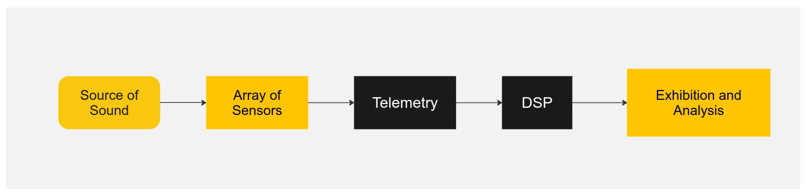
The acoustic signal acquired by the SoNaR was processed to detect possible targets, as it is shown in Figure 1. Ship classification indicates potential threats to early warning systems. The accurate classification of encountered vessels enables the planning of appropriate measures to effectively mitigate threats. A human SoNaR operator often faces uncertainty when classifying contacts, which may hinder appropriate actions. A possible solution is to use a support system fed by the signal to extract features for classifying the contacted ship.

Trained operators often detect and categorize submarine threats using low-frequency analysis and recording (Lofar) displays of spectral and temporal profiles of passive SoNaR waves [10]. Submarine defense depends greatly on SoNaR-based surveillance, and it may be significantly improved by automatic models that recognize the target from its acoustic signature.

A class-modular Multi-Layer Perceptron (MLP) network reported a ship classification accuracy of 93% in [1], whose analysis was based on real signals produced by eight vessel classes. Passive SoNaR target classification using an MLP trained with the salp swarm algorithm achieved an accuracy of 97.12% in [11], where the signals were made in a closed water circuit cavitation tunnel (https://www.sciencedirect.com/topics/engineering/cavitation-tunnel accessed on 10 January 2025) model NA-10 England, when three classes were simulated. An unsupervised generative framework utilizing a variational autoencoder (VAE) was proposed to create more disentangled representations for downstream classification tasks in [2], which obtained F1 scores much greater than 0.9 for most of the ten target classes.

Few signals are typically available to train classifiers due to the operational difficulty of recording diverse vessel scenarios and the classified nature of military SoNaR data. Since these recordings often contain sensitive acoustic signatures, they are restricted as part of broader national security protocols. When the amount of data is limited, generative adversarial networks (GANs) can be used [12] to synthesize numerous passive SoNaR records and train Convolutional Neural Networks (CNNs).

This study evaluated the accuracy of seven different ML techniques for ship classification using SoNaR data. The primary objective was to develop and assess an ML model that integrates real characterization data from static and moving ships. We employed eXtreme Gradient Boost (XGBoost) and Linear Discriminant Analysis (LDA) to model this scenario and compare their performances with a Support Vector Machine (SVM), K-Nearest Neighbors (KNN), and ridge regression [13,14,15]. Data preprocessing could be conducted with signal compression using Principal Component Analysis (PCA) [16].

The main contributions of this study are summarized as follows:

• A comparative evaluation of seven machine learning algorithms for ship classification using real-world passive SoNaR data.
• The inclusion of LDA and XGBoost, which were not previously applied in this context, as strong candidates for real-time, accurate classification.
• A detailed investigation into the effect of preprocessing techniques—such as decimation, TPSW, and PCA—on the models’ performances.
• The construction of a balanced dataset from real static and dynamic operations that involved 12 ships of the Brazilian Navy.

The remainder of this paper is organized as follows: Section 2 presents the preprocessing pipeline and SoNaR signal transformations. Section 3 details the machine learning models employed. Section 4 outlines the experimental setup and evaluation methodology. Section 5 discusses the results, and Section 6 concludes with final remarks and future directions.

Decimation techniques may be used on the raw data to optimize the system performance. Our aim was to evaluate the effectiveness and robustness of the evaluated algorithms in static and dynamic contexts, focusing on learning and identifying significant patterns and enhancing the prediction accuracy for real-world measurements.

The resulting classifier was trained and evaluated using target records acquired during several data collection expeditions, one for each vessel, conducted by the Brazilian Navy at the Brazilian Operating Systems Support Center (CASOP) in the Arraial do Cabo litoral area.

The dataset consisted of acoustic noise signals corresponding to 12 ships in a 1500-meter-long shallow water route in a controlled environment. The acoustic emissions of the ships were recorded under various operational and machinery circumstances, that is, several ship runs for different boats. Data were collected at two different moments: a stationary scenario with the anchored ship, denoted as static, and, subsequently, in a moving scenario within the area of the acoustic ray, denoted as dynamic. A hydrophone, which was positioned at a depth of 45 m, recorded the sound using a 22,050 Hz sampling frequency and 8-bit resolution. Recording began when the ship was 1000 m before passing the hydrophone, and the recording ended when the ship was 500 m after the hydrophone.

This study implemented both static and dynamic data characterization for ships, providing more accurate insights for analysis. An acoustic signature of a ship refers to the unique sound patterns it produces, which is used for detection and identification. There are two types: static and dynamic. The static acoustic signature consists of sounds generated when the ship is stationary or moving at a constant speed, including noises from the hull, onboard machinery, and propulsion system. These signatures are relatively constant and easier to analyze. In contrast, the dynamic acoustic signature involves sounds produced while the ship is in motion, such as noise from the propulsion system, interactions between the hull and water, and changes in operational activities. Dynamic signatures vary with speed, course, and operational conditions, making them more complex and harder to predict. Additionally, we advanced the use of other ML techniques, such as XGBoost and topic modeling through LDA, which transforms data into a domain where classes can be separated.

Another contribution of this work was the data preprocessing stage, in which different dimensionality reduction techniques were applied. This study explored the impact of decimation and non-decimation on the performance of these techniques and analyzed their effects on both the effectiveness and efficiency of the proposed characterization. In summary, this study offered a comprehensive critical view of the various stages of SoNaR data processing for ML models and this paper presents alternatives for optimizing the modeling process.

2. Preprocessing Chain for SoNaR Signals

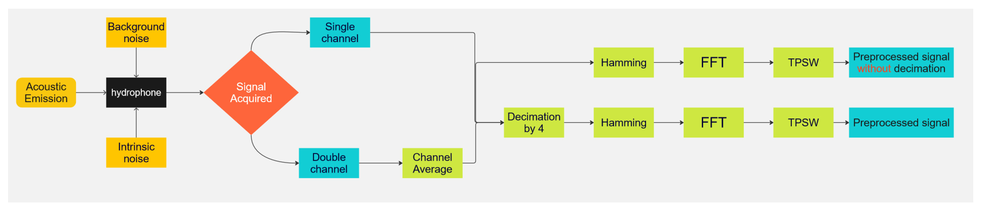
When data are acquired, the raw data may be incomplete, redundant, or noisy, and data preprocessing techniques are then used to mitigate such problems [17]. Figure 2 shows the processing pipeline employed to extract the information presented to the classification models from the passive radar records.

2.1. Lofar

Low-frequency analysis and recording (Lofar) is a method for extracting the parameters of a time–frequency representation of the incoming SoNaR signal. Lofar involves creating a time–frequency representation of the input signal windowed to smooth spectral leakage. In this study, we used a Hamming window to generate the Lofar [18].

A fast Fourier transform (FFT) is applied to windowed signal blocks to transform the signal into the frequency domain. This results in the lofargram representing the frequency magnitude along the time in the signal acquisition bearing, that is, the azimuth. A lofargram denotes a time–frequency representation of the signal, which is represented graphically with the frequency on the vertical axis and the time on the horizontal axis. If there are multiple hydrophones, then different bearings can result in different lofargrams.

The magnitude of the Lofar of a signal may be significant for machine learning classifiers. Large peaks indicate the presence of high-signal components. Nevertheless, background noise must be whitened to facilitate the search for signals [19]. Before the Lofar can be used for classification, it is processed using a two-pass split window (TPSW) to mitigate the effects of noise [20].

The acoustic signature of ship machinery typically spans frequencies up to 5 kHz [21]. Working with the correct frequency band [21] ensures efficient processing and focuses on the relevant information.

The audio signal must be represented using a fast Fourier transform (FFT) [22]. This involves representing the waveform of the signal with a discrete vector sampled at specific times with a sampling interval $T_s$ and a sampling frequency $f_s=1/T_s$ that exceeds the Nyquist frequency. The sampling rates used were 1411 and 2116 kbit/s to record the frequencies of 44 kHz and 66 kHz, respectively.

To provide adequate resolution of the signal spectrum, 2048 points were used to represent the entire frequency band. When a 66 kHz sampling rate was used, the first 1870 points covered the band from 0 to 6 kHz, while the first 280 points covered the same range for 44 kHz, which slightly exceeded a 5 kHz range of interest. Considering the potentially higher sampling rates in the future, we worked with the first 400 frequency lines. The idea is to work with signals captured from different sources in the future, either from a hydrophone or SoNaR. Nevertheless, 400 samples still constituted many attributes, which increased the classifier’s computational complexity and stabilized the model learning, but required a large dataset to train the models effectively. To address this challenge, dimensionality reduction techniques were explored to simplify the problem and reduce the computational complexity while retaining essential information. Specifically, Principal Component Analysis (PCA) and Nonlinear Principal Component Analysis (NLPCA) techniques were evaluated for preprocessing.

2.2. Data Preprocessing Stages

In the preprocessing flow diagram presented in Figure 2, data discretization involves converting continuous data into discrete data, which is essential for machine learning classification. Data transformation consists of converting data from one format or structure to an alternative format that is more suitable for analysis, storage, or processing. This process includes normalization, scaling, coding, filling in missing data, and identifying features from the original data. Data cleaning aims to correct or remove incorrect, corrupted, incorrectly formatted, or duplicate data from a dataset. If the data are noisy, then the models and results may be unreliable. Data cleaning techniques were employed depending on the dataset and noise characteristics.

The signal-processing chain is shown in Figure 2, which follows [23] with some adaptions to certain characteristics of our dataset. A pipeline without decimation was implemented in this work, which attempted to retain more signals and aggregate frequency information. The signal was captured by a hydrophone with intrinsic noise from the environment and equipment. Signals could be recorded in either mono or 2-channel stereo. The average of the channels was computed for the stereo signals. In the first pipeline, the signals were decimated by a factor of four, which reduced the time resolution. The signals were then converted to a lower sampling rate while preserving their main characteristics. In the second pipeline, the signals were not decimated. This approach was used to evaluate the impact of decimation on a smaller resolution in the spectrum. The acoustic signature was recorded in a 22 kHz audio format and then reduced to 5.5 kHz or recorded at 16 kHz and reduced to 4 kHz by decimation.

2.3. Two-Pass Split Window

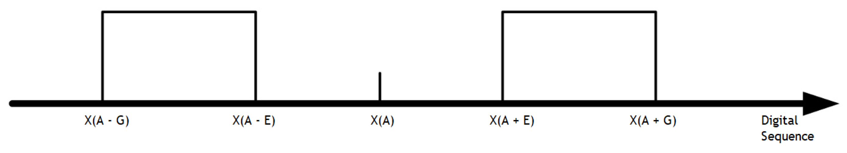
The TPSW is a noise-whitening technique [20,24]. Let $\mathbf{X}=\left[\begin{array}{cccc}X\left(1\right),& X\left(2\right),& \dots ,& X\left(N\right)\end{array}\right]$, where $X\left(i\right)$ represents the absolute value on the $i^{\mathrm{th}}$ frequency beam of the Lofar and N is the length. The TPSW estimates the noise level of interest $X\left(\gamma \right)$, where $\gamma =1,2,\dots ,N$, using the spectral lines inside the two neighboring windows, as illustrated in Figure 3.

The indices of the samples in Figure 3, taking A as the center of the window, that is, ($X_{A-G}$ to $X_{A-E}$) in the left window and ($X_{A+G}$ to $X_{A+E}$) in the right window, are $X_A=\left\{X_i\right|i=A+k,k\in \{-G,-G+1,\dots ,-E,E,E+1,\dots ,G\}\}.$ Note that when index i is close to the beginning or near the end of the data support, the corresponding window is truncated at the boundaries of the sequence. The local average of the elements inside the two windows is

$$\mu \left(A\right)=\sum _{i\in {\mathcal{X}}_A}{\displaystyle \frac{{\mathbf{X}}_i}{A}}.$$

(1)

The TPSW takes advantage of the average noise ${\mu }_A$, which is a function of the neighborhood of the frequency bin A. To estimate ${\mu }_A$ to properly filter the noise, the sequence

$$\Phi \left(A\right)=\left\{\begin{array}{cc}X\left(A\right)\hfill & \mathrm{if}X\left(A\right)<r\tilde{X}\left(A\right)\hfill \\ \tilde{X}\left(A\right)\hfill & \mathrm{if}X\left(A\right)\ge r\tilde{X}\left(A\right)\hfill \end{array}\right.,$$

(2)

is used, where $r=1+C{[(4/\pi -1)/A]}^{1/2}$, $C\ge 1$ is a constant, and $A=G-E+1$ is the window length. The normalized TPSW is given by

$$Z_{\mathrm{TPSW}}\left(A\right)={\displaystyle \frac{X\left(A\right)}{\mu \left(A\right)}}.$$

(3)

After this chain of procedures, the feature data were used to feed the classifier.

2.4. Database Balancing and Partitioning

The Brazilian Navy provided a database for acoustic signals through the CASOP Military Organization. Hydrophones were installed on the sea floor to record the acoustic signatures of ships traveling along the Arraial do Cabo lane. The sound records are stored and cataloged in a database.

The dataset contains static recordings, with the stalled ship’s equipment operational under normal conditions, and dynamic recordings, i.e., with ships actively moving within the acoustic lane.

The data records contain static instances of docked ships with equipment turned on and systems online, such as auxiliary combustion engines and water chiller units. The boat moved to the sea, and its acoustic signature was recorded in this dynamic situation with the equipment online. A ship sometimes used two main combustion engines, whereas the ship used just one engine in others. A distinct acoustic signature was obtained for each configuration.

The original database comprises measurements for 12 ships of different types, with different durations and numbers of races per ship. Some recordings from the dynamic phase are longer than forty-five minutes, while others from the static phase are shorter than forty seconds.

The greatest number of dynamic races per ship is five, and some ships present only one dynamic race, but a greater number of static races. To counteract the varying numbers of runs and the different run durations, the database was balanced.

From the previous description of acquired data, one readily sees that the database should be balanced. The database was balanced so that M distinct signatures from each ship were available while prioritizing the diversity of ship signals. Seven banks or subsets of segmented race blocks were created and merged from the original dataset of races to create a dataset that contained 40 signals for each vessel, or 480 signals, if decimation was not used. This bank prioritized different ship runs and parts of the same run, where each of them lasted four seconds, as depicted in

Table 1. Segmented databases.

Bank 1	Data
A1	0–40 s
A2	0–40 s
A3	0–40 s
A4	0–40 s
B1	0–40 s
C1	0–40 s
C2	0–40 s
Bank 2	Data
A1	40–80 s
A2	40–80 s
A3	40–80 s
A4	40–80 s
B1	40–80 s
C1	40–80 s
C2	40–80 s
Bank 3	Data
A1	80–120 s
A2	80–120 s
A3	-
A4	80–120 s
B1	80–120 s
C1	80–120 s
C2	80–120 s
Bank 4	Data
A1	-
A2	120–160 s
A3	-
A4	-
B1	120–160 s
C1	-
C2	120–160 s
Bank 5	Data
A1	-
A2	160–200 s
A3	-
A4	-
B1	160–200 s
C1	-
C2	-
A1	-
A2	200–240 s
A3	-
A4	-
B1	200–240 s
C1	-
C2	-
A1	-
A2	240–280 s
A3	-
A4	-
B1	240–280 s
C1	-
C2	-

.

In Bank 1, as depicted in Table 1, our aim was to identify four distinct signatures for each ship. For the A signal, all four signatures were located in Bank 1. The process began by reading and registering A1, followed by incrementing the line counter. Subsequently, A2 was processed, and this continued until A4 was registered. At this point, the signal counter reached its maximum value or overflowed. Upon overflowing, the system proceeded to search for the next signal.

Moving to the B signal, as the line counter incremented, a comparison revealed a different signal C1. Consequently, the database counter was incremented and moved to Bank 2. The process repeated for B1’ to B1”’, where it spanned Banks 2 to 4. Upon reading the fourth signal, the signal counter overflowed, which prompted the search for the next signal to commence in the first bank.

Proceeding to the C signal in Bank 1, only two signatures were present. After registering C1 and incrementing the line counter, C2 was processed. Since no further C signals were available, the database counter was incremented, which shifted to Bank 2. This cycle continued until all relevant signals were registered, which resulted in the creation of an equiprobable database, as illustrated in

Table 2. Equiprobable database segmentation.

Equiprobable Database	Time Interval
A1	0–40 s
A2	0–40 s
A3	0–40 s
A4	0–40 s
B1	0–40 s
B1’	40–80 s
B1”	80–120 s
B1”’	120–160 s
C1	0–40 s
C2	0–40 s
C1’	40–80 s
C2’	40–80 s

.

This database is not available for research because it contains the acoustic signatures of the Brazilian Navy, which has not authorized its availability to the general public.

2.5. DataFrame TPSW

The transformations performed in the signals from the bank of runs were implemented in Python to generate the DataFrame TPSW. The resulting DataFrame had 480 entries, and it was balanced to include 40 entries for each of the 12 classes when decimation was present. When decimation was not performed, 5760 entries were used, with 480 entries for each vessel. Each input was represented by a 2048-point vector derived from the fast Fourier transformed magnitude, which was whitened using the TPSW technique. This generated the DataFrame TPSW, which served as an appropriate input for the ML algorithms. Their results were placed in a DataFrame, which is defined as a set of two-dimensional tabular data that are changeable in size and potentially heterogeneous, which allows for flexibility. It has a data structure containing labeled axes, rows, and columns, where arithmetic operations are aligned on row and column labels.

2.6. Principal Component Analysis

PCA represents a set of vectors using a subspace spanned by the singular vectors of incoming data. PCA can be used to reduce data dimensions when data features are highly correlated, making the data more suitable for regression and classification models that generally assume independence between the features [25]. The limitations of PCA lie in its assumption of linearity [26] when selecting an appropriate number of principal components capable of representing the data with a definable reconstruction error and loss of interpretability of the original characteristics.

PCA normalizes the dataset to ensure that each variable has a mean of 0 and a standard deviation equal to 1 so that each variable contributes equally. This reduces the sensitivity to the differences between the variances of the original variables. Significant differences may lead to biased results [26]. Transforming the data into an adequate excursion range avoids this problem.

The cross-covariance matrix between the feature vectors $\mathbf{x}$ and the class labels $\mathbf{y}$ is expressed by ${\Sigma }_{(\mathbf{x},\mathbf{y})}={\displaystyle \frac{1}{n-1}}{\sum }_{i=1}^n({\mathbf{x}}_i-{\mu }_x){({\mathbf{y}}_i-{\mathit{\mu }}_y)}^T,$ where ${\mathbf{x}}_i$ is the i-th observation of the feature vector, ${\mathbf{y}}_i$ is the i-th observation of the class labels, ${\mathit{\mu }}_x$ is the mean vector of the features, ${\mathit{\mu }}_y$ is the mean vector of the class labels, and n is the number of observations.

The principal components were derived from eigendecomposition of the autocovariance matrix. The eigenvectors were organized in the decreasing order of the associated eigenvalues, which formed the feature vectors [26]. Most of the information within the original variables is usually concentrated into a few significant components. The principal components comprise a new basis on which the differences between the original observations may become more evident. They represent the directions of the data subspace with maximum variance [26].

Kernel Nonlinear Principal Component Analysis (Kernel NLPCA) extends the PCA algorithm to capture the nonlinear relations between variables and uses a more compact representation via a kernel. In a higher-dimensional feature space, features may be linearly separated. Subsequently, the use of a higher-dimensional feature space reduces the number of attributes to be evaluated.

In some applications, there may be a database with many features, and applying transformations that involve many polynomial combinations of these features can lead to extremely high and impractical computational costs. A kernel trick provides a solution to this problem. The trick represents the data only through similarity comparisons and vector products in pairs with the original data $\mathbf{x}$, relating them to the original coordinates in the lower-dimensional space, and those projected in the larger space instead of explicitly applying the transformations, i.e., $k(\mathbf{x},y)=\langle \mathit{\varphi }\left(\mathbf{x}\right),\mathit{\varphi }\left(y\right)\rangle ,$ in which $\langle ·,·\rangle$ is the inner product, $\mathbf{x},y\in \mathbf{X}$ is the space spanned by the data vectors, and $\mathit{\varphi }:X\to {\mathbb{R}}^n$ is the kernel. The data are projected into a high-dimensional space, but the new space is not explicitly calculated; only its inner products are. The nonlinear mappings of features in a higher dimension can separate data that are inseparable in lower dimensions.

After preprocessing the SoNaR acoustic signals, the resulting data were presented for the ship classification. Seven ML algorithms were tested to evaluate the best learned to correctly assign the ship class from the feature vector.

3. Classifier Models

In this study, seven classifiers were considered. Five of them have been used for underwater acoustic signal classification. To the best of our knowledge, LDA and XGBoost have been used for ship classification.

3.1. Multi-Layer Perceptron

A Multi-Layer Perceptron (MLP) is composed of an input layer, one or more hidden layers, and an output layer [1]. Each layer consists of neurons that perform transformations on the data via weighted sums and activation functions.

Given an input vector $\mathbf{x}=[x_1,x_2,\dots ,x_n]$, the output of the j-th hidden neuron is computed using

$$z_j=\sum _{i=1}^n{w}_{ji}{x}_i+b_j,h_j=f\left(z_j\right),$$

where $w_{ji}$ are the weights, $b_j$ the bias, and f an activation function (e.g., sigmoid or ReLu [27]).

The output layer receives the transformed values $h_j$ and computes

$$y_k=g\left(\sum _{j=1}^m{v}_{kj}{h}_j+c_k\right),$$

where $v_{kj}$ and $c_k$ are the weights and biases of the output layer, and g is the output activation function (e.g., softmax for classification or linear for regression).

3.2. K-Nearest Neighbors

The K-Nearest Neighbors (KNN) algorithm classifies a new data point based on the K closest training samples using a distance metric, most commonly the Euclidean distance [28]. KNN is a non-generalizing learning method, as it stores all training data and it does not involve an explicit training phase.

The distance between two points $\mathbf{x}$ and $\mathbf{y}$ is defined as

$$d(\mathbf{x},\mathbf{y})={\left(\sum _{i=1}^n{x}_i-y_i^p\right)}^{1/p},$$

which generalizes several metrics, including Euclidean ($p=2$), Manhattan ($p=1$), and Minkowski distances.

The value of K influences the model behavior: small values make it sensitive to noise, while larger values provide smoother predictions but may overlook local patterns. Once the K nearest neighbors are identified, the predicted class $\widehat{y}$ for a query point $\mathbf{x}$ is given by a majority vote:

$$\widehat{y}=arg\underset{c}{max}\sum _{i=1}^K\mathbb{I}(y_i=c),$$

where $\mathbb{I}(y_i=c)$ is the indicator function, which is equal to 1 if $y_i=c$, and 0 otherwise. The class with the most votes is assigned to the query point.

3.3. Ridge Regression

Ridge regression is a linear regression that adds a regularization term to ordinary least squares (OLS) regression to prevent overfitting by penalizing large coefficients, which is an extension of OLS with ${\mathsf{\ell }}_2$ regularization [29]. In linear regression, the goal is to find the coefficients $\beta$ that minimize the sum of the squared differences between the actual and predicted values. The objective function for OLS is

$$\mathrm{Min}{\displaystyle \frac{1}{n}}\sum _{i=1}^n{(y_i-{\widehat{y}}_i)}^2={\displaystyle \frac{1}{n}}\sum _{i=1}^n{(y_i-X_i\beta )}^2,$$

where $y_i$ is the actual value of the target variable, ${\widehat{y}}_i=X_i\beta$ is the predicted value (with $X_i$ being the vector of input features for sample i, and $\beta$ the coefficient vector), and n is the number of samples. This minimizes the residual sum of squares (RSS); however, if there are highly correlated features or a small dataset, OLS tends to overfit, leading to large unstable coefficients.

Ridge regression addresses the overfitting problem by adding a penalty term to the OLS objective function. This penalty is proportional to the square of the magnitude of the coefficients; that is, ${\mathsf{\ell }}_2$ regularization:

$$\mathrm{Min}{\displaystyle \frac{1}{n}}\sum _{i=1}^n{(y_i-X_i\beta )}^2+\lambda \sum _{j=1}^p{\beta }_j^2,$$

$\lambda$ is a regularization parameter that controls the strength of the penalty, ${\beta }_j$ are the coefficients of the regression model, and p is the number of features.

The objective is a combination of fitting the model to minimize the sum of squared errors (SSR) and penalizing the size of the coefficients ${\beta }_j^2$ so that the large coefficients shrink toward zero.

3.4. Logistic Regression

Logistic regression is a statistical model used for binary classification in which the output is a categorical variable with two possible outcomes. A logistic regression estimates the probability of an event occurring [30]. It is based on the logistic function, also known as the sigmoid function, which maps any real-valued number into the range $(0,1)$ and allows logistic regression to output probabilities. The logistic function is given by

$$\sigma \left(z\right)={\displaystyle \frac{1}{1+e^{-z}}},$$

where $z=X\beta$, X is a linear combination of input features, $\beta$ are the model coefficients, and e is the base of the natural logarithm. This function takes any value of z, which can range from $-\infty$ to ∞, and compresses it in the range $(0,1)$. For logistic regression, z represents the log odds of the target variable being one.

In logistic regression, we model the log odds of the event, that is, the logarithm of the ratio between the probability of success and the probability of failure, as a linear function of the input features:

$$log\left({\displaystyle \frac{P(y=1\mid X)}{1-P(y=1\mid X)}}\right)=X\beta ,$$

(4)

where $P(y=1\mid X)$ is the probability of the event occurring (the output being 1), X is the matrix of input features, and $\beta$ is the vector of coefficients.

The left-hand side of Equation (4) shows the log odds, and its right-hand side shows a linear combination of the input features. Taking the exponential on both sides yields

$${\displaystyle \frac{P(y=1\mid X)}{1-P(y=1\mid X)}}=e^{X\beta }.$$

Solving this equation for $P(y=1\mid X)$, we obtain the logistic regression model

$$P(y=1\mid X)={\displaystyle \frac{1}{1+e^{-X\beta }}},$$

which represents the probability that the outcome is 1 given the input features.

Once the probability $P(y=1\mid X)$ is calculated, we can make the following prediction:

• If $P(y=1\mid X)\ge 0.5$, $y=1$ is predicted;
• If $P(y=1\mid X)<0.5$, $y=0$ is predicted.

To fit the logistic regression model, we estimate the coefficients $\beta$. This is achieved by minimizing a cost function that measures the difference between the predicted probabilities and actual labels. For logistic regression, the cost function is the log loss or binary cross-entropy:

$$J\left(\beta \right)=-{\displaystyle \frac{1}{n}}\sum _{i=1}^n\left[y_{i}log\left(P(y_i\mid X_i)\right)+(1-y_i)log(1-P(y_i\mid X_i))\right],$$

where $y_i$ is the actual label for sample i, $P(y_i\mid X_i)$ is the predicted probability for sample i, and n is the number of samples.

The log-loss function penalizes incorrect predictions more heavily, as the predicted probability diverges from the true label.

Gradient descent is typically used to find the optimal coefficients $\beta$ because the cost function in logistic regression is nonlinear. Gradient descent iteratively updates (represented by the symbol: =) the coefficients by moving in the direction of the negative gradient of the cost function:

$$\beta :=\beta -\alpha {\displaystyle \frac{\partial J\left(\beta \right)}{\partial \beta }},$$

where $\alpha$ is the learning rate, which controls the step size, and ${\displaystyle \frac{\partial J\left(\beta \right)}{\partial \beta }}$ is the gradient of the cost function with respect to $\beta$. The gradient descent continues until the convergence criterion is satisfied.

Similar to linear regression, regularization can be added to logistic regression to prevent overfitting. The two common types of regularization are as follows:

• ${\mathsf{\ell }}_2$ regularization (ridge) adds a penalty term that is proportional to the square of the coefficients:

  $$J\left(\beta \right)=-{\displaystyle \frac{1}{n}}\sum _{i=1}^n\left[y_{i}log\left(P(y_i\mid X_i)\right)+(1-y_i)log(1-P(y_i\mid X_i))\right]+{\displaystyle \frac{\lambda }{2}}\sum _{j=1}^p{\beta }_j^2;$$
• ${\mathsf{\ell }}_1$ regularization (Lasso) adds a penalty proportional to the absolute value of the coefficients:

  $$J\left(\beta \right)=-{\displaystyle \frac{1}{n}}\sum _{i=1}^n\left[y_{i}log\left(P(y_i\mid X_i)\right)+(1-y_i)log(1-P(y_i\mid X_i))\right]+\lambda \sum _{j=1}^p{\beta }_j.$$

Here, $\lambda$ controls the regularization strength. Regularization reduces overfitting by constraining the size of the coefficients.

3.5. Support Vector Machine

A Support Vector Machine (SVM) uses support vectors to classify and obtain comparisons between the support vectors and the class of the input to be predicted. It can perform binary and multiclass classification on a dataset [27].

Suppose we have a dataset with N training examples $({\mathbf{x}}_i,y_i)$, where ${\mathbf{x}}_i\in {\mathbb{R}}^n$ is an input feature vector with n dimensions and $y_i\in \{-1,1\}$ is the class label for each input (1 or −1).

The goal of the SVM is to find a hyperplane that separates the data points such that the margin, that is, the distance between the hyperplane and the nearest data points from each class, is maximized. A hyperplane is defined as the set of points $\mathbf{x}$ that satisfy the following equation:

$${\mathbf{w}}^T\mathbf{x}+b=0,$$

where $\mathbf{w}\in {\mathbb{R}}^n$ is a vector that is normal to the hyperplane, and $b\in \mathbb{R}$ is the bias term.

The decision function for predicting the class of a new input $\mathbf{x}$ is

$$f\left(\mathbf{x}\right)=\mathrm{sign}({\mathbf{w}}^T\mathbf{x}+b).$$

If $f\left(\mathbf{x}\right)>0$, class $+1$ is predicted, and class $-1$ is predicted otherwise.

3.6. Linear Discriminant Analysis

LDA is a classifier with a linear decision boundary that is generated by adjusting class-conditional densities to the data using Bayes’ theorem. The model adjusts the estimated density curve for each class assuming that all classes share the same covariance matrix [14].

LDA aims to find a linear combination of features that separates two or more classes. In a two-class problem, LDA determines the optimal direction that maximizes the distance between the means of the two classes while minimizing the variance within each class. Consider a dataset with N samples, each with n features, denoted as

$$\mathbf{X}=[{\mathbf{x}}_1,{\mathbf{x}}_2,\dots ,{\mathbf{x}}_N],$$

where ${\mathbf{x}}_i\in {\mathbb{R}}^n.$ Suppose the dataset comprises two classes, $y\in \{0,1\}$, where each class has $N_0$ and $N_1$ data points, respectively. LDA finds a linear discriminant direction $\mathbf{w}$ such that the projected data ${\mathbf{w}}^T\mathbf{x}$ achieve the best separation between the two classes.

Two matrices are key to this method: the within-class scatter matrix $S_w$ and the between-class scatter matrix ${\mathbf{S}}_b$. ${\mathbf{S}}_w$ measures how much the data points vary within each class. For the two classes, $S_w$ is defined as follows:

$${\mathbf{S}}_w=\sum _{i=1}^{N_0}({\mathbf{x}}_i-{\mu }_0){({\mathbf{x}}_i-{\mu }_0)}^T+\sum _{i=1}^{N_1}({\mathbf{x}}_i-{\mu }_1){({\mathbf{x}}_i-{\mu }_1)}^T$$

where ${\mu }_0$ and ${\mu }_1$ are the mean vectors of classes 0 and 1, respectively:

$${\mu }_0={\displaystyle \frac{1}{N_0}}\sum _{i=1}^{N_0}{\mathbf{x}}_i,{\mathit{\mu }}_1={\displaystyle \frac{1}{N_1}}\sum _{i=1}^{N_1}{\mathbf{x}}_i,$$

and ${\mathbf{S}}_b$ measures the spread between the mean vectors of the classes. It is defined as

$${\mathbf{S}}_b=({\mathit{\mu }}_1-{\mathit{\mu }}_0){({\mathit{\mu }}_1-{\mathit{\mu }}_0)}^T,$$

where ${\mathit{\mu }}_0$ and ${\mathit{\mu }}_1$ denote the mean vectors of the two classes.

The goal of LDA is to determine the direction $\mathbf{w}$ that maximizes the separation between classes. Specifically, LDA maximizes the ratio of the between-class to within-class scatter. This ratio can be expressed as follows:

$$J\left(\mathbf{w}\right)={\displaystyle \frac{{\mathbf{w}}^T{\mathbf{S}}_b\mathbf{w}}{{\mathbf{w}}^T{\mathbf{S}}_w\mathbf{w}}}.$$

Maximizing this ratio ensures that the distance between the class means is large, while keeping the variance within each class small. The optimization problem leads to the following generalized eigenvalue problem [14]:

$${\mathbf{S}}_w^{-1}{\mathbf{S}}_b\mathbf{w}=\lambda \mathbf{w}.$$

The solution $\mathbf{w}$ is the eigenvector corresponding to the largest eigenvalue $\lambda$, which provides the direction that maximizes the class separability. Once the optimal projection vector $\mathbf{w}$ is obtained, the data points are projected onto $\mathbf{w}$, i.e., $z={\mathbf{w}}^T\mathbf{x}$. LDA makes predictions by classifying a data point $\mathbf{x}$ into one of two classes based on the position of its projection z relative to a threshold. The threshold was computed as the midpoint between the projected means of the two classes.

For a new point $\mathbf{x}$, the classification rule is

$$y=\left\{\begin{array}{cc}0,\hfill & \mathrm{if}{\mathbf{w}}^T\mathbf{x}<t,\hfill \\ 1,\hfill & \mathrm{if}{\mathbf{w}}^T\mathbf{x}\ge t,\hfill \end{array}\right.$$

where t is the threshold often chosen as the midpoint of the projected class mean.

3.7. eXtreme Gradient Boosting

XGBoost builds an incremental model and progressively enables optimization of arbitrary differentiable loss functions. At each stage, n regression trees are adjusted in the direction opposite to the gradient of the loss function. Binary classification is a special case in which only a single regression tree is used [13].

XGBoost is an ensemble learning method in which multiple weak learners, such as decision trees, are trained sequentially, and the model is optimized from the errors made by previous learners. The objective function in XGBoost comprises two terms:

$$\mathrm{Obj}\left(\theta \right)=\sum _{i=1}^{n}L(y_i,{\widehat{y}}_i)+\sum _{k=1}^K\Omega \left(f_k\right),$$

where $L(y_i,{\widehat{y}}_i)$ is the loss function that measures the extent to which prediction ${\widehat{y}}_i$ matches the actual value $y_i$. This can be the mean squared error (MSE) for regression or log loss for classification, and $\Omega \left(f_k\right)$ is the regularization term that penalizes the complexity of each individual tree $f_k$, preventing overfitting. For trees, this term usually measures the number of leaves and the ${\mathsf{\ell }}_2$ norm of leaf weights as follows:

$$\Omega \left(f\right)=\gamma T+{\displaystyle \frac{1}{2}}\lambda \sum _{j=1}^T{w}_j^2,$$

where T is the number of leaves in the tree, $w_j$ are the weights of the leaves, and $\gamma$ and $\lambda$ are the hyperparameters that control the regularization.

XGBoost is an additive model in which predictions are built iteratively. Starting with an initial prediction ${\widehat{y}}^{\left(0\right)}$, new trees are added to improve the predictions:

$${\widehat{y}}^{\left(t\right)}={\widehat{y}}^{(t-1)}+f_t\left(x\right)$$

where $f_t\left(x\right)$ is the tree added at step t, which aims to correct the errors from the previous step. Each tree attempts to minimize the residual errors from the previous iteration.

The XGBoost algorithm iteratively uses gradient descent to minimize the objective function. Specifically, it computes the pseudo-residuals, which are the negative gradients of the loss function with respect to the current predictions:

$$r_i^{\left(t\right)}=-{\displaystyle \frac{\partial L(y_i,{\widehat{y}}_i^{(t-1)})}{\partial {\widehat{y}}_i^{(t-1)}}}.$$

These residuals $r_i^{\left(t\right)}$ serve as the targets for the next tree to predict. The tree is fitted to minimize these residuals using a loss function, such as the MSE.

XGBoost uses a second-order Taylor expansion of the loss function to optimize it effectively:

$$L(y_i,{\widehat{y}}_i^{\left(t\right)})\approx L(y_i,{\widehat{y}}_i^{(t-1)})+g_i{f}_t\left(x_i\right)+{\displaystyle \frac{1}{2}}{h}_i{f}_t{\left(x_i\right)}^2,$$

where $g_i={\displaystyle \frac{\partial L(y_i,{\widehat{y}}_i^{(t-1)})}{\partial {\widehat{y}}_i^{(t-1)}}}$ is the first-order gradient and $h_i={\displaystyle \frac{{\partial }^{2}L(y_i,{\widehat{y}}_i^{(t-1)})}{\partial {\widehat{y}}_i^{{(t-1)}^2}}}$ is the second-order derivative.

The goal is to find a tree $f_t\left(x\right)$ that minimizes this approximation of the loss.

The algorithm builds decision trees by splitting the data at different points based on feature values. The gain $G_s$ for each possible split was computed as follows:

$$G_s={\displaystyle \frac{1}{2}}\left[{\displaystyle \frac{G_L^2}{H_L+\lambda }}+{\displaystyle \frac{G_R^2}{H_R+\lambda }}-{\displaystyle \frac{{(G_L+G_R)}^2}{H_L+H_R+\lambda }}\right]-\gamma ,$$

where $G_L$ and $G_R$ are the sums of gradients for the left and right splits; $H_L$ and $H_R$ are the sums of Hessians for the left and right splits; $\lambda$ is the regularization parameter; and $\gamma$ is the penalty for each split, that is, regularization.

Regularization is a key feature of XGBoost. It controls the complexity of the trees, prevents overfitting, and ensures that the model generalizes well. Regularization is achieved through the parameters $\gamma$ to control the number of splits and $\lambda$ to control the magnitude of the leaf weights.

After training multiple trees, the final prediction for a sample was obtained by summing the predictions from all trees as follows:

$$\widehat{y}=\sum _{t=1}^T{f}_t\left(x\right),$$

where $f_t\left(x\right)$ denotes the prediction from the t-th tree.

Among the seven algorithms used, logistic regression cannot be supported without due treatment in the multiclass case. However, it can be used if certain techniques are applied, such as one against all and one against one.

3.8. Binary Classifiers for Multiclass Problems

Some classifiers are designed to perform binary classification tasks that distinguish between only two classes: y and $\overline{y}$. To extend these techniques to multiclass problems, two strategies are commonly employed: one against one and one against all [31]:

• One against one: If there are $\gamma$ classes, then $\left[\gamma \right(\gamma -1\left)\right]/2$ binary classifiers are trained. Each classifier distinguishes between two specific classes from $\gamma$ possible classes. For example, for three classes $y_A$, $y_B$, and $y_C$, three binary classifiers are implemented: $C_{y_A}\times C_{y_B}$, $C_{y_A}\times C_{y_C}$, and $C_{y_B}\times C_{y_C}$. Each classifier makes a prediction and the input is classified based on the class with the most votes among the outputs.
• One against all: $\gamma$ binary classifiers are trained, where each of them distinguishes between one class and the others. For example, with three classes $y_A$, $y_B$, and $y_C$, three binary classifiers are implemented: $C_{y_A}\times \left(C_{y_{(B+C)}}\right)$, $C_{y_B}\times \left(C_{y_{(A+C)}}\right)$, and $C_{y_C}\times \left(C_{y_{(A+B)}}\right)$. Each model predicts a probability score for the membership of the class, and the class with the highest score is selected as the prediction.

3.9. Parameters of the Models

This subsection discusses the relevant methodological aspects used to evaluate the performance of an ML algorithm. For the proper evaluation, the database DataFrame TPSW was divided into distinct sets that were used to train, validate, and test the ML models. We used the K-fold cross-validation technique, which increases the reliability of the performance assessment by carefully partitioning the database.

Classification involves assigning a class y from a set of predefined classes to the input data $\mathbf{x}$; that is, it is the mapping from the input features $\mathbf{x}$ to one of the classes y. Some classification models are based on regression, where the regression ML model learns to predict mapping from the input features to a continuous target variable [27].

Labeled data with the correct output were used in the supervised learning paradigm to train the ML model. The model learns to map the input to the output based on examples provided during training [27].

To identify the most efficient and effective approach, some ML models were evaluated to determine which yielded the best results from the data. The analyses considered the original data and its decimated version, which were filtered using TPSW, in addition to PCA and NLPCA compression.

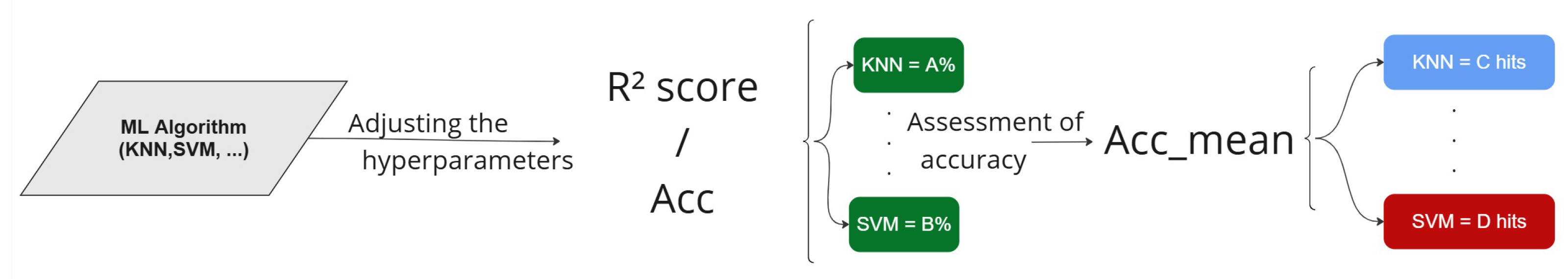
As a criterion for evaluating machine learning models, the metric $R^2$ score was used for the regressors, whereas accuracy (Acc) was used for the classifiers. This provides a strategy for developing a classification algorithm tailored to the dataset. Once each model was optimized, its performance was evaluated based on the accuracy of the predicted class, measured by the accuracy metric ${\left\{Acc\right\}}_t$, which is the total number of correct predictions over the total number of predictions across several epochs. Figure 4 illustrates the process.

4. Methodology of the Design and Evaluation of the Classifiers

Various metrics were used to assess the performance of the models and algorithms. The metrics were chosen based on the type of problem to be solved.

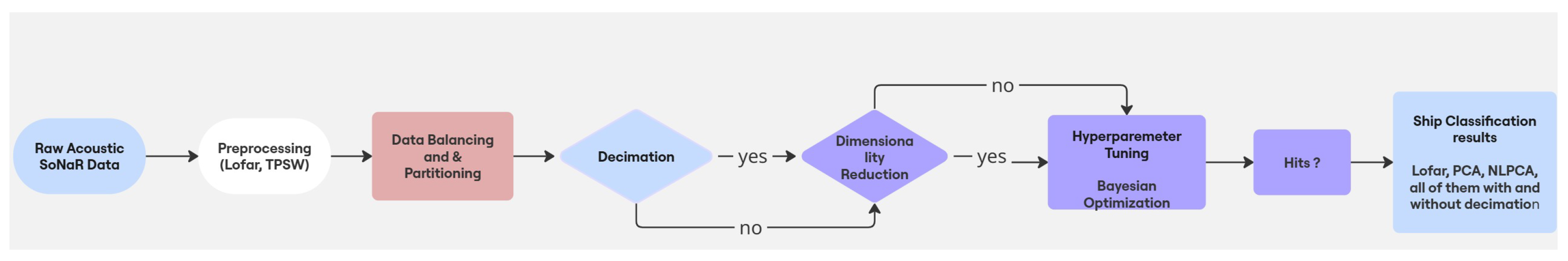
The methodology proposed for ship classification using passive SoNaR signals consists of a structured pipeline involving several stages, as illustrated in the flowchart in Figure 5. The process begins with the acquisition of raw acoustic data and progresses through signal processing, dimensionality reduction, model training, and evaluation.

1. Raw Acoustic SoNaR Data

The input into the system consisted of raw underwater acoustic signals captured from a set of ships that operated under different conditions (e.g., static and dynamic scenarios). These signals were the basis for the subsequent processing steps.

2. Preprocessing (Lofar, TPSW)

The raw signals were transformed into time–frequency representations using the Lofar technique, which enhanced the visibility of tonal components in the signal. Additionally, the two-pass split window (TPSW) algorithm was applied to perform noise whitening and improve the signal quality by reducing the background noise and interference.

3. Dimensionality Reduction (PCA/NLPCA)

Following the preprocessing and optional decimation, the data underwent dimensionality reduction using either Principal Component Analysis (PCA) or Nonlinear PCA (NLPCA). These techniques were used to reduce the feature space while retaining the most significant information, which improved the generalization and reduced the overfitting in the machine learning models.

4. Decimation

At this stage, a decision was made whether to apply decimation to the preprocessed signals. Decimation reduces the sampling rate, lowering computational costs while potentially affecting the resolution of the relevant signal features. The methodology evaluated both the decimated and non-decimated paths in parallel to determine their impacts on the performance.

5. Data Balancing and Partitioning

The dataset was then balanced to ensure an equal number of samples for each ship class. This step was crucial to avoid bias during model training. The data was partitioned into training, validation, and test sets to allow for proper evaluations of the models.

6. Hyperparameter Tuning (Bayesian Optimization)

Machine learning models were trained using optimized hyperparameters obtained through Bayesian optimization. This method provided an efficient way to explore the parameter space and select the best configurations for performance.

7. Accuracy Evaluation

The trained models were evaluated using cross-validation to estimate their generalization capability. Metrics such as accuracy and statistical confidence intervals (e.g., mean plus/minus standard deviation) were calculated to assess the model performance. The metric “Hits” refers to the successful predictions across folds.

8. Ship Classification Results

The final stage aggregates the results from all pipelines—Lofar, PCA, and NLPCA—each tested with and without decimation. This comprehensive comparison allowed for the identification of the most effective preprocessing and modeling strategy for the ship classification.

4.1. Metrics for Evaluating Classification

Considering the nature of the experimental design, in which we constructed 1000 models per algorithm through repeated executions, a purely statistical approach became the most appropriate and informative method for analysis. Therefore, while the confusion matrix played a fundamental role in deriving the per-model results, our emphasis in the manuscript was on the statistical summary of these results to provide a more robust and generalizable performance evaluation of the algorithms under study.

The accuracy is the proportion of correctly classified instances relative to the total number of instances. The accuracy was used to evaluate the classifiers. It is dependent on the number of hits A and the total of events T, as defined by

$$Acc={\displaystyle \frac{A}{T}},$$

(5)

The scalar for Acc was obtained by training the same ML algorithm. Although, the division of data signals into the test, training, and validation sets was random, the balance between the quantity of signals in each set was maintained, but the division is random. Therefore, the learning of different relations $(\mathbf{x},y)$ probably occurred, possibly leading to different responses for the regressor and, consequently, for Acc.

One way to achieve this inaccuracy is to train the same algorithm with different training and test set segmentations. To achieve this, a k-fold was used. Assuming a Gaussian distribution for accuracy, with mean $\overline{Acc}$, it is possible to estimate the confidence interval ${\mathbf{Acc}}_t$ of the classification of the same ML algorithm trained T times with the same database. The accuracy confidence interval is a function of the average accuracy $\overline{Acc}$ and the standard deviation z, where

$$\overline{Acc}={\displaystyle \frac{1}{n}}\sum _{i=1}^N{\mathrm{Acc}}_i,$$

(6)

and the interval

$$\overline{Acc}\pm (z·\mathrm{SE}),$$

(7)

such that z is the number of standard deviations that a value is away from the mean of the normal distribution, where SE is the standard error of the estimated parameter. For a 95% confidence interval, z is approximately 1.96.

Using accuracy as the average of the confidence interval, we obtain

$$\mathrm{SE}=\sqrt{{\displaystyle \frac{1}{n}}\mathrm{Acc}(1-\mathrm{Acc})}.$$

(8)

Therefore,

$${\mathrm{Acc}}_t=\mathrm{Acc}\pm z\sqrt{{\displaystyle \frac{A}{n}}\mathrm{Acc}(1-\mathrm{Acc})},$$

(9)

where the accuracy is measured in a classification epoch, that is, each of the k-folds, using the cross-validation methodology, and ${\mathrm{Acc}}_t$ is the average of Acc over all epochs.

4.2. Hyperparameter Tuning and Evaluation

A search was performed to determine the set of hyperparameters that led to reliable models in terms of $R^2$ via Bayesian optimization. The final models were trained with optimized hyperparameters, which were further tested with a set of attributes for classification.

A model suffers from overfitting when it fits the training data excessively, capturing noise or random fluctuations instead of the underlying patterns between $\mathbf{x}$ and y. In this case, the model performed well on the training data, but it generally failed to generalize to unseen data; an overfitting machine presents high accuracy on training data but low accuracy on validation or test data. Avoiding overfitting and underfitting involves finding a suitable model complexity and regularization level, leading to a good generalization performance on unknown data. Regularization techniques, model selection, and thorough evaluation are crucial for mitigating these issues and building effective generalization models.

The causes of overfitting include complex models with too many parameters relative to the amount of training data, a poor choice of feature vectors contaminated with noisy or irrelevant data, and insufficient parameter tuning [27]. Underfitting occurs when a model is too simple to capture the relationships between $\mathbf{x}$ and y.

To mitigate the risk of overfitting and underfitting, several strategies were adopted throughout the training and evaluation of the machine learning models. First, a repeated 10-fold cross-validation procedure was implemented, which resulted in 1000 models per classifier. This robust validation strategy ensured that the performance estimates reflected a wide variety of data partitions, which improved the generalization and reduced the dependency on any specific subset of the dataset.

Second, we computed the confidence intervals for classification accuracy using standard error propagation under the assumption of a Gaussian distribution. This allowed us to quantify performance variability and provided insight into the stability of each model.

Third, to prevent the models from overfitting the training data, we employed Bayesian hyperparameter optimization, which included regularization parameters such as $\alpha$, C, and $\lambda$. These hyperparameters were tuned independently for each model and dataset variation, which ensured that the model complexity was adequately controlled.

Additionally, dimensionality reduction techniques were applied to decrease the feature space dimensionality. PCA and NLPCA were used to retain only the most informative components of the acoustic features, particularly when dealing with high-resolution lofargrams. This step was critical in minimizing the risk of overfitting due to high-dimensional input vectors.

Although the dataset was relatively small compared with deep learning benchmarks, it was structured, labeled, and balanced after preprocessing and segmentation, which ranged from 480 to 5760 instances depending on the configuration. These conditions made it suitable for training and evaluating classical machine learning algorithms. The combination of balanced data, regularized models, and conservative validation strategies supported the reliability of the findings presented in this study.

By analyzing the influence of hyperparameters on a given machine’s training process and learning, each of the seven tested classifiers had its own set of hyperparameters that should be tuned for each of the six data frames to lead to a reliable training process, and thus, adequate models.

In the case of the XGBoost classifier, which employs sequential decision trees using regression residuals from previous trees, optimizing hyperparameters such as the contribution of each tree to the final response and the depth of the tree branches is crucial. Extremely deep trees can lead to overfitting because they may subdivide classes into increasingly smaller groupings that are not necessarily relevant to the question at hand.

Bayesian optimization is a technique for model optimization based on Bayes’ theorem [32], which describes the a posteriori probability $P\left(AB\right)$ of an event A conditioned on another event B given the probabilities of the individual events $P\left(A\right)$ and $P\left(B\right)$ and the probability of the conditioned event $P\left(BA\right)$. In hyperparameter optimization, Bayesian optimization seeks to find the set of hyperparameters that maximizes a chosen figure of merit, such as the $R^2$ score. This requires defining a suitable search space for the hyperparameters and creating a probabilistic model for the set of hyperparameters based on the chosen metric.

Bayesian optimization iteratively selects the best set of hyperparameters by updating the estimated probabilities based on past evaluations. This results in a stochastic search [32], in which the probability density of the search space is adjusted according to the observed performance of the model during the search.

Bayesian optimization requires a defined stopping criterion. In this study, a minimum of 30 epochs were initially adopted, with halting imposed if there was an increase of less than 1% in the figure of merit after testing ten additional points. If the $R^2$ score did not exhibit increasing behavior, additional points were tested until improvement was observed, up to a maximum of 100 additional points.

In this study, we employed the Gaussian Naive Bayes classifier due to its computational efficiency and effectiveness in handling continuous data. Gaussian Naive Bayes assumes that the features follow a Gaussian distribution within each class, which aligns well with the statistical properties of the acoustic features extracted from the Lofar spectrograms. This probabilistic approach allows the model to estimate the likelihood of each class based on observed feature values, making it particularly suitable for classification tasks where the independence assumption between features is reasonable. Additionally, its fast training and prediction times make it a practical choice for real-time or resource-constrained operational environments, such as those encountered in naval passive SoNaR applications [33].

4.3. Dataset Partitioning

It is essential to divide the dataset into multiple subsets. The most common approach involves splitting the data into two or three parts: a training set and a test set, or a training, validation, and test set.

The training set is used to teach the model by providing input–output examples, specifically, for pairs of independent variables $\mathbf{x}$ and the dependent variable y. Through this, the model learns the underlying patterns and relationships.

The validation set is used to monitor the model’s performance during training. It helps evaluate the generalization of the model to new data and prevents overfitting by tuning parameters and selecting the best model.

The test set contains data that the model has never seen during training or validation. It is used for the final evaluation, providing an unbiased estimate of the model’s real-world performance.

There is ongoing debate over how best to split the data. A common rule of thumb is to allocate 70% of the data for training, and 15% each for validation and testing [34].

To better evaluate a model’s stability and generalization, cross-validation techniques are often used. In K-fold cross-validation, the dataset is divided into K folds. For each of the K epochs, one fold is used as the test set, while the remaining $K-1$ folds are used for training and validation. This process ensures that every data point is used for testing exactly once.

If the model’s performance is consistent across all K epochs, it suggests that the model is stable and performs similarly on unseen data. The final model performance is typically taken as the average of the K results.

5. Results

Through experimentation and evaluation, the strengths and limitations of each algorithm for ship classification were demonstrated under varying conditions. This clarified their effectiveness in handling high-dimensional datasets and feature spaces when working with the Lofar database, as well as low-dimensional scenarios when data compression techniques, such as PCA and NLPCA, were applied. The reliability of the different methodologies was validated through extensive experimentation using 10-fold cross-validation. Each algorithm was executed 100 times, which resulted in a total of 1000 models per machine learning technique, with the average accuracy scores ($\overline{Acc}$) calculated.

To illustrate the results, six representative graphs are presented, all of which were based on signals without decimation. For testing 1000 models after all the hyperparameters were defined, the execution time was 0:04:59.806241 per machine learning algorithm. Once a model was trained, the execution time for processing 40 inputs was only 0:00:00.134981. This demonstrates the feasibility of applying the methodology in operational scenarios.

Figure 6 and Figure 7 present a histogram and kernel density estimation (KDE) curve to illustrate the distribution of the accuracy values, where all of them are for signals without decimation. The red curve represents the density estimate, providing a smoothed approximation of the distribution of accuracy values. The x-axis represents the accuracy. The histogram, shown by gray bars, indicates the frequency of the accuracy values.

To visualize the results, all of them using validation data, we generated graphs that illustrated the distribution of the accuracy values across multiple runs. The key parameters extracted from these graphs include the mean accuracy and standard deviation, which indicate the stability of the performance of the model. In addition, we included density distributions to observe the variations in accuracy.

Although more than 42 graphs were obtained with Lofar, PCA, and NLPCA, each one with and without decimation and for two machines using the one × one and one × all, for brevity, we present only six representative graphs: Figure 6 and Figure 7. This provides a clear and concise overview of the model’s behavior, helping to better understand its performance characteristics.

5.1. Multi-Layer Perceptron

The optimal hyperparameters for each model were determined using the method described in Section 4.2.

Table 3. MLP hyperparameters and model’s performance for the Lofar, PCA, and NLPCA variations of the database.

Hyperparameter	Lofar		PCA		NLPCA
	w/ Dec	w/o Dec.	w/ Dec	w/o Dec.	w/ Dec	w/o Dec.
$\alpha$ (Regularization Parameter)	0.001	0.001	0.002711	0.002711	0.0656	0.0656
Number of Neurons in Hidden Layer	58 units	58 units	95 units	95 units	100 units	100 units
Initial Learning Rate	0.00117	0.00117	0.00431	0.00431	0.00369	0.00369
Maximum Number of epochs	100	100	967	967	100	100
Solver	Adam	Adam	Adam	Adam	Adam	Adam
Mean Accuracy $\overline{Acc}$	0.123	0.363	0.437	0.437	0.553	0.437
Standard Error (SE)	$5.96·{10}^{-2}$	$5.64·{10}^{-2}$	$4.51·{10}^{-2}$	$4.51·{10}^{-2}$	$6.08·{10}^{-2}$	$4.51·{10}^{-2}$

presents the selected hyperparameters and classification results for the MLP models trained on different database variations. These results highlight the extent to which the input dimensionality could hinder the model performance. In contrast, the models trained on the dimensionally reduced datasets (PCA and NLPCA) achieved approximately 10% higher accuracies, indicating improved performances.

When examining the average accuracy and standard deviation across the 30-fold cross-validation, the results are consistent with the reported accuracy values ($\mathrm{Acc}$). While the optimal hyperparameters differ between the Lofar, PCA, and NLPCA variations, they appeared similar owing to the rounding. It is important to note, however, that the models trained on the PCA and NLPCA data were more complex, with significantly more neurons in the hidden layer.

The MLP model’s performance, measured by the accuracy, decreased with the application of decimation across all the database variations, with Lofar showing the largest drop. PCA and NLPCA performed similarly, with NLPCA showing slightly better performance with and without decimation. The hyperparameters, particularly the regularization parameter, number of neurons, and learning rate, were tailored for each variation; however, the model’s performance did not seem to benefit significantly from these adjustments in this specific case.

5.2. K-Nearest Neighbors

The hyperparameters that best fit the model and corresponding classification results are presented in

Table 4. KNN hyperparameters and the model’s performance for the Lofar, PCA, and NLPCA variations of the database.

Hyperparameter	Lofar		PCA		NLPCA
	w/ Dec	w/o Dec.	w/ Dec	w/o Dec.	w/ Dec	w/o Dec.
Neighbors	1	1	2	2	2	2
Weights	Distance	Distance	Distance	Distance	Distance	Distance
Mean Accuracy $\overline{Acc}$	0.996	0.578	0.578	0.996	0.578	0.996
Standard Error (SE)	$2.67·{10}^{-3}$	$7.91·{10}^{-2}$	$7.91·{10}^{-2}$	$2.67·{10}^{-3}$	$7.91·{10}^{-2}$	$2.76·{10}^{-3}$

.

The KNN classifier performed well without decimation, where it achieved an almost perfect accuracy (99.6%) across all dataset variations (Lofar, PCA, and NLPCA). However, decimation significantly impacted the model’s performance, where the accuracy dropped to 0.58 for all the datasets when decimation was applied. The hyperparameters of the model, such as the number of neighbors and the use of the Manhattan distance with distance-based weights, were consistent across all the datasets, ensuring a fair comparison.

The confusion matrix in Figure 8 for the KNN classifier with Lofar without decimation demonstrates excellent overall performance, with a total of 1203 correct predictions out of 1211 samples. Most classes were classified with perfect accuracy, as evidenced by the strong diagonal dominance in the matrix. The only notable misclassifications occurred in class 0, where eight samples were incorrectly predicted as belonging to class 5. This suggests a possible similarity or overlap in the feature space between these two classes.

5.3. Ridge

The hyperparameters that best fit the ridge model and resulting classification results are listed in

Table 5. Ridge hyperparameters and the model’s performance for the Lofar, PCA, and NLPCA variations of the database.

Hyperparameter	Lofar		PCA		NLPCA
	w/ Dec	w/o Dec.	w/ Dec	w/o Dec.	w/ Dec	w/o Dec.
$\alpha$ (Regularization Parameter)	1	1	10	10	10	10
$\gamma$ (Regularization Parameter)	Distance	Distance	Distance	Distance	Distance	Distance
Kernel	Linear	Linear	Linear	Linear	Linear	Linear
Mean Accuracy $\overline{Acc}$	0.958	0.530	0.578	0.530	0.578	0.530
Standard Error (SE)	$1.18·{10}^{-3}$	$6.94·{10}^{-2}$	$7.91·{10}^{-2}$	$6.94·{10}^{-2}$	$7.91·{10}^{-2}$	$6.94·{10}^{-2}$

. The analysis of the acoustic signature classification results using ridge regression indicated the model’s ability to generalize to unknown data, where it achieved an accuracy of 96%.

Decimation significantly improved the mean accuracy, with the Lofar’s going from 0.48 to 0.96, and PCA/NLPCA’s from 0.53 to 0.97. This proved that decimation was crucial for improving the model performance. The NLPCA and PCA variations show similar results, with mean accuracies of 0.97 with decimation and 0.53 without it. Lofar, while still benefiting from decimation, had a lower performance in both the decimated and non-decimated cases. The standard errors (SEs) were much smaller for the PCA and NLPCA datasets with decimation (0.02) than for Lofar (0.08), indicating that decimation led to more stable results for the PCA and NLPCA models.

5.4. Support Vector Machine

Table 6. SVM (one × one) configurations with Lofar, PCA, and NLPCA.

Hyperparameter	Lofar		PCA		NLPCA
	w/ Dec	w/o Dec.	w/ Dec	w/o Dec.	w/ Dec	w/o Dec.
C (Regularization Parameter)	393,520	393,520	114,026	114,026	114,026	114,026
Loss	Hinge	Hinge	Squared hinge	Squared hinge	Squared hinge	Squared hinge
Penalty	${\mathsf{\ell }}_2$	${\mathsf{\ell }}_2$	${\mathsf{\ell }}_2$	${\mathsf{\ell }}_2$	${\mathsf{\ell }}_2$	${\mathsf{\ell }}_2$
Mean Accuracy $\overline{Acc}$	0.517	0.612	0.515	0.0753	0.515	0.0753
Standard Error (SE)	$8.38·{10}^{-2}$	$3.44·{10}^{-2}$	$8.35·{10}^{-2}$	$1.18·{10}^{-2}$	$8.35·{10}^{-2}$	$1.18·{10}^{-2}$

presents the optimal hyperparameters and the corresponding classification results for the SVM models.

The SVM model showed a relatively consistent performance across the Lofar, PCA, and NLPCA datasets, as represented in

Table 7. SVM (one × all) configurations with Lofar, PCA, and NLPCA.

Hyperparameter	Lofar		PCA		NLPCA
	w/ Dec	w/o Dec.	w/ Dec	w/o Dec.	w/ Dec	w/o Dec.
C (Regularization Parameter)	393,520	393,520	114,026	114,026	114,026	114,026
Loss	Hinge	Hinge	Squared hinge	Squared hinge	Squared hinge	Squared hinge
Penalty	${\mathsf{\ell }}_2$	${\mathsf{\ell }}_2$	${\mathsf{\ell }}_2$	${\mathsf{\ell }}_2$	${\mathsf{\ell }}_2$	${\mathsf{\ell }}_2$
Mean Accuracy $\overline{Acc}$	0.467	0.0896	0.469	0.562	0.469	0.529
Standard Error (SE)	$9.02·{10}^{-2}$	$2.14·{10}^{-2}$	$9.54·{10}^{-2}$	$4.27·{10}^{-2}$	$9.54·{10}^{-2}$	$2.97·{10}^{-2}$

. The accuracy of the model decreased significantly when decimation was applied; however, this reduction was consistent across all the datasets. The regularization parameter CC for Lofar was much larger than that for PCA and NLPCA, indicating a stronger regularization applied for Lofar, but this did not lead to a major difference in the performance of the model. Without decimation, the model achieved stable and consistently high accuracy across the datasets. The slight differences in the hyperparameters, such as the loss function and C, did not seem to have a major impact on the overall performance in this case.

The results indicate that the Lofar dataset without decimation performed notably poorly, where it achieved a mean accuracy of only 8.92%. This suggests that the raw high-dimensional signal substantially hindered the SVM classification ability. Although decimation improved the performance in the Lofar dataset, where it yielded a moderate accuracy of 46.7%, it remained inferior compared with the results obtained from PCA and NLPCA. In contrast, both PCA and NLPCA benefited from the absence of decimation, likely owing to their reduced dimensionality and more structured data representation. Additionally, it was observed that standard errors were generally higher in the decimated models, particularly for Lofar and PCA, indicating greater variability in the model performance across the folds.

5.5. Logistic Regression

The hyperparameters that best fit the logistic regression model (one × one) were identified, and the classification results are presented in

Table 8. Logistic regression (one × one) hyperparameters and the model’s performance for the Lofar, PCA, and NLPCA variations of the database.

Hyperparameter	Lofar		PCA		NLPCA
	w/ Dec	w/o Dec.	w/ Dec	w/o Dec.	w/ Dec	w/o Dec.
C (Regularization Parameter)	1.361	1.361	0.766	0.766	0.7661	0.7661
Solver	Liblinear	Liblinear	Liblinear	Liblinear	Liblinear	Liblinear
Penalty	${\mathsf{\ell }}_1$	${\mathsf{\ell }}_1$	${\mathsf{\ell }}_1$	${\mathsf{\ell }}_1$	${\mathsf{\ell }}_1$	${\mathsf{\ell }}_1$
Mean Accuracy $\overline{Acc}$	0.932	0.917	0.972	0.995	0.972	0.995
Standard Error (SE)	$4.21·{10}^{-2}$	$4.42·{10}^{-2}$	$4.42·{10}^{-3}$	$2.70·{10}^{-2}$	$4.42·{10}^{-3}$	$2.69·{10}^{-3}$

. Similarly, the results of the logistic regression (one × all) are shown in

Table 9. Logistic regression (one × all) hyperparameters and the model’s performance for the Lofar, PCA, and NLPCA variations of the database.

Hyperparameter	Lofar		PCA		NLPCA
	w/ Dec	w/o Dec.	w/ Dec	w/o Dec.	w/ Dec	w/o Dec.
C (Regularization Parameter)	14.503	14.503	0.822	0.822	0.822	0.822
Solver	Liblinear	Liblinear	Liblinear	Liblinear	Liblinear	Liblinear
Penalty	${\mathsf{\ell }}_1$	${\mathsf{\ell }}_1$	${\mathsf{\ell }}_1$	${\mathsf{\ell }}_1$	${\mathsf{\ell }}_1$	${\mathsf{\ell }}_1$
Mean Accuracy $\overline{Acc}$	0.917	0.995	0.929	0.995	0.929	0.995
Standard Error (SE)	$4.42·{10}^{-2}$	$2.63·{10}^{-3}$	$4.08·{10}^{-3}$	$2.53·{10}^{-3}$	$4.08·{10}^{-3}$	$2.53·{10}^{-3}$

.

While the results obtained with the SVM show that linearly separating the data into classes was not easy, the results achieved with the logistic regression emphasize that using a nonlinear kernel leveraged the model performance. With a few parameters to be optimized, significant results were achieved using the logistic regression classifier.

The logistic regression (one × one) model performed excellently with 99.5% accuracy when no decimation was applied and had a slightly reduced accuracy (approximately 92–93%) with decimation. The performances across the three dataset variations (Lofar, PCA, and NLPCA) were very similar, indicating that the model’s behavior was consistent across these variations. The regularization parameter C was slightly higher for Lofar, but this did not seem to affect the performance noticeably. The model was highly stable and consistent, with very low standard errors for both with and without decimation, particularly when no data reduction was applied.

The logistic regression model using the one × all classification strategy showed an excellent performance, with a 99% accuracy without decimation across all the datasets. With decimation, the accuracy decreased slightly (92% for Lofar and 93% for PCA and NLPCA), indicating that decimation had a small negative impact on the performance. However, the overall performance remained high for all the datasets, with very low standard errors, indicating consistent and stable predictions.

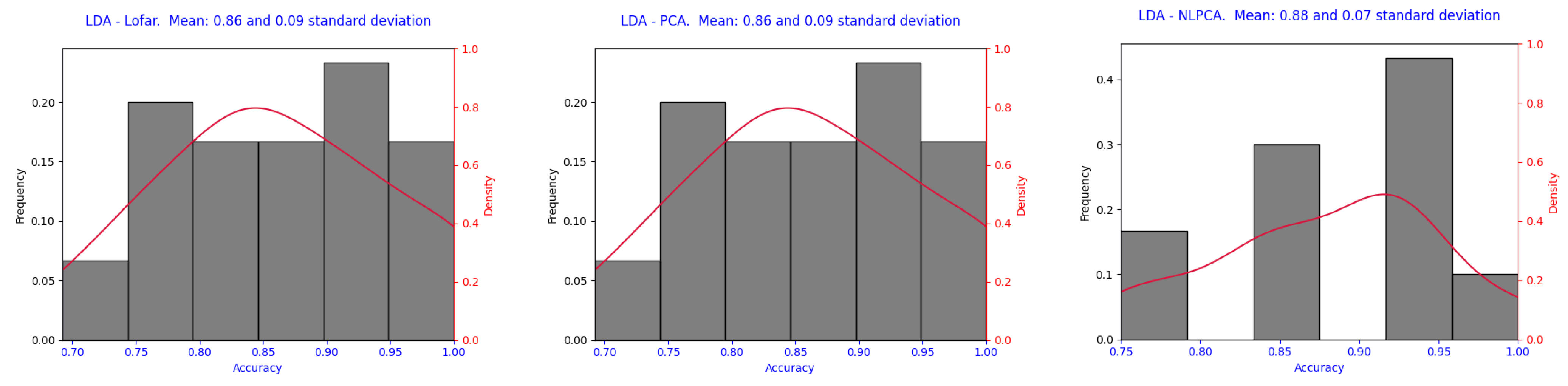
5.6. Linear Discriminant Analysis

When using the Lofar signal as a feature vector, the LDA classifier was expected to perform well because the number of classes was inherently embedded within the structure of the signal. This suggests that the Lofar signal serves as an ideal discriminant when classes are well separated. The optimal hyperparameters for each model are listed in

Table 10. LDA hyperparameters and the model’s performance for the Lofar, PCA, and NLPCA variations of the database.

Hyperparameter	Lofar		PCA		NLPCA
	w/ Dec	w/o Dec.	w/ Dec	w/o Dec.	w/ Dec	w/o Dec.
Components	10	10	5	5	5	5
Solver	SVD	SVD	SVD	SVD	SVD	SVD
Mean Accuracy $\overline{Acc}$	0.859	0.995	0.859	0.995	0.859	0.995
Standard Error (SE)	$8.39·{10}^{-2}$	$4.69·{10}^{-3}$	$8.39·{10}^{-2}$	$4.69·{10}^{-3}$	$8.39·{10}^{-2}$	$4.69·{10}^{-3}$

to maximize the performance.

The LDA classifier performed very well, where it achieved a 0.99 accuracy without decimation for all the dataset variations (Lofar, PCA, and NLPCA). The model was slightly impacted by decimation, where the mean accuracy dropped to 0.86 for Lofar and PCA and 0.90 for NLPCA. However, the performance remained robust across all the datasets, where NLPCA demonstrated a marginally better ability to handle decimation. The consistency of the model was also high, as reflected by the low standard errors. The choice of 10 components for Lofar and 5 for PCA and NLPCA seemed appropriate and did not significantly affect the overall performance.

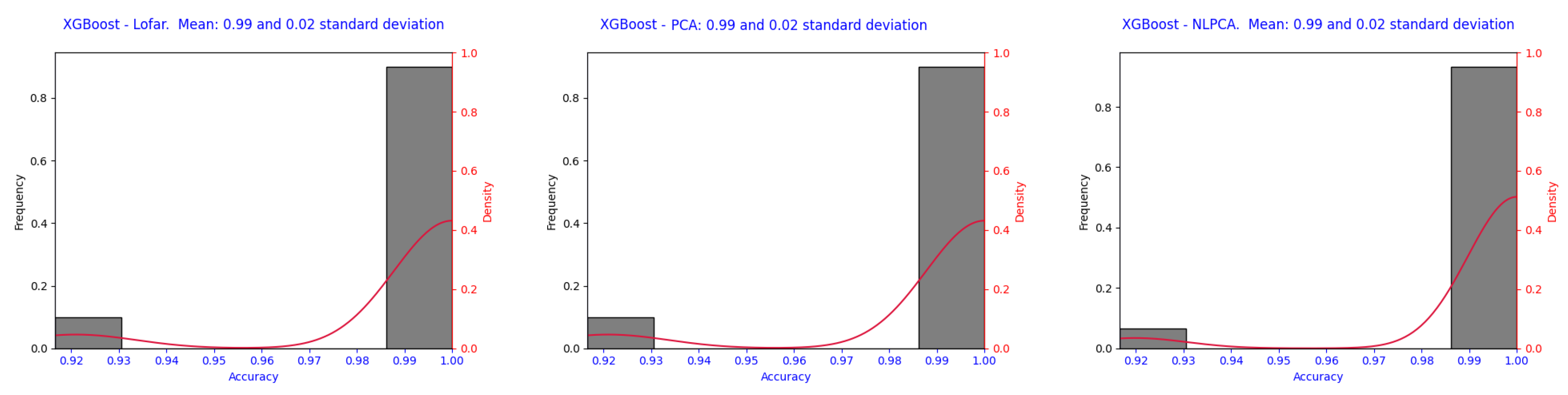
5.7. XGBoost

The hyperparameters that best fit the XGBoost model were found, and the classification results are presented in

Table 11. XGBoost hyperparameters and the model’s performance for the Lofar, PCA, and NLPCA variations of the database.

Hyperparameter	Lofar		PCA		NLPCA
	w/ Dec	w/o Dec.	w/ Dec	w/o Dec.	w/ Dec	w/o Dec.
alpha	${10}^{-6}$	${10}^{-6}$	$1.359·{10}^{-5}$	$1.359·{10}^{-5}$	${10}^{-6}$	${10}^{-6}$
colsample_bytree	0.934	0.934	1.0	1.0	0.470	0.470
gamma	1	1	${10}^{-6}$	${10}^{-6}$	0.0603	0.0603
lambda	1	1	$3.637·{10}^{-6}$	$3.637·{10}^{-6}$	1	1
learning_rate	0.051	0.051	0.245	0.245	0.01	0.01
max_depth	10	10	1	1	3	3
min_child_weight	4	4	4	4	1	1
n_estimators	1000	1000	560	560	849	849
subsample	1.0	1.0	0.937	0.937	0.426	0.426
Mean Accuracy $\overline{Acc}$	0.997	0.996	0.886	0.994	0.997	0.997
Standard Error (SE)	$1.38·{10}^{-2}$	$4.61·{10}^{-3}$	$1.38·{10}^{-2}$	$5.75·{10}^{-3}$	$1.38·{10}^{-2}$	$3.66·{10}^{-3}$

. Subsequently, the machine was trained and tested on a separate dataset, which yielded the results shown in Figure 7.

The general result of 99% accuracy with a standard deviation of 0.02% demonstrated the good performance of this technique, which worked with a series of classifying trees for residues. Such an accuracy is adequate for using this model in practical cases.

Achieving a high accuracy across multiple tests indicates that the model generalized well to unknown data. This suggests that the model learned meaningful patterns from the training data that were applied to new, unseen examples. The model performed consistently well across multiple subsets of data, with a high accuracy maintained across the different separations of the data, which indicates its generalization capacity.

5.8. Comparison of Machine Learning Models for Classification

In this subsection, we compare the performances of the seven (MLP, KNN, ridge, SVM, logistic regression (one × one and one × all), LDA, and XGBoost) machine learning models for the classification task. The objective was to evaluate the effectiveness of each model in accurately classifying the target variables and identifying the most appropriate model.

Table 12. Mean accuracy ($\overline{Acc}$) and standard error (SE) for each model using Lofar, PCA, and NLPCA datasets, both with and without decimation.

Model	Lofar		PCA		NLPCA
	$\overline{\mathit{Acc}}$	SE	$\overline{\mathit{Acc}}$	SE	$\overline{\mathit{Acc}}$	SE
With Decimation
MLP	0.123	$5.96·{10}^{-2}$	0.437	$4.51·{10}^{-2}$	0.553	$6.08·{10}^{-2}$
KNN	0.996	$2.67·{10}^{-3}$	0.578	$7.91·{10}^{-2}$	0.578	$2.76·{10}^{-3}$
Ridge	0.958	$1.18·{10}^{-3}$	0.578	$7.91·{10}^{-2}$	0.578	$7.91·{10}^{-2}$
SVM (OvO)	0.517	$8.38·{10}^{-2}$	0.515	$8.35·{10}^{-2}$	0.515	$8.35·{10}^{-2}$
SVM (OvA)	0.467	$9.02·{10}^{-2}$	0.469	$9.54·{10}^{-2}$	0.469	$9.54·{10}^{-2}$
Logistic Regression (OvO)	0.932	$4.21·{10}^{-2}$	0.972	$4.42·{10}^{-3}$	0.972	$4.42·{10}^{-3}$
Logistic Regression (OvA)	0.917	$4.42·{10}^{-2}$	0.929	$4.08·{10}^{-3}$	0.929	$4.08·{10}^{-3}$
LDA	0.859	$8.39·{10}^{-2}$	0.859	$8.39·{10}^{-2}$	0.859	$8.39·{10}^{-2}$
XGBoost	0.997	$1.38·{10}^{-2}$	0.886	$1.38·{10}^{-2}$	0.997	$1.38·{10}^{-2}$
Without Decimation
MLP	0.363	$5.64·{10}^{-2}$	0.437	$4.51·{10}^{-2}$	0.437	$4.51·{10}^{-2}$
KNN	0.578	$7.91·{10}^{-2}$	0.996	$2.67·{10}^{-3}$	0.996	$2.76·{10}^{-3}$
Ridge	0.530	$6.94·{10}^{-2}$	0.530	$6.94·{10}^{-2}$	0.530	$6.94·{10}^{-2}$
SVM (OvO)	0.612	$3.44·{10}^{-2}$	0.0753	$1.18·{10}^{-2}$	0.0753	$1.18·{10}^{-2}$
SVM (OvA)	0.0896	$2.14·{10}^{-2}$	0.562	$4.27·{10}^{-2}$	0.529	$2.97·{10}^{-2}$
Logistic Regression (OvO)	0.917	$4.42·{10}^{-2}$	0.995	$2.70·{10}^{-2}$	0.995	$2.69·{10}^{-3}$
Logistic Regression (OvA)	0.995	$2.63·{10}^{-3}$	0.995	$2.53·{10}^{-3}$	0.995	$2.53·{10}^{-3}$
LDA	0.995	$4.69·{10}^{-3}$	0.995	$4.69·{10}^{-3}$	0.995	$4.69·{10}^{-3}$
XGBoost	0.996	$4.61·{10}^{-3}$	0.994	$5.75·{10}^{-3}$	0.997	$3.66·{10}^{-3}$

summarizes the results and Figure 9 elucidates them better.

The results with decimation yielded higher-performance models, such as XGBoost, ridge, and logistic regression, which showed the highest accuracies across the preprocessing methods, where they achieved over 96% accuracy. On the other hand, lower-performance models, such as SVM and MLP, achieved accuracies below 60%. These models generally showed a higher standard deviation with decimation, indicating less repeatability in the performances across different runs.

The performance without decimation resulted in a significant improvement, where KNN and logistic regression (both types) achieved a 100% accuracy across all the preprocessing methods. This suggests that having less-spread data significantly aided in stabilizing and improving the performance. Conversely, for MLP, the accuracy decreased across the board, which might suggest overfitting issues or a poor interaction between the model complexity and reduced data variance through decimation. Moreover, a notable decrease in the standard deviation for most models indicates an increased consistency in the results with decimation.

The results with decimation were faster because they involved fewer data points, which facilitated the discovery of a relationship between the feature vector x and predicted class $y_p$. The standard deviation was directly related to the preprocessing chain, which affected the consistency and variability of the model outcomes. This understanding should help in selecting appropriate models and preprocessing methods for tasks where the model stability and high accuracy are crucial, particularly in scenarios where data variance is a concern.

In the area of feature vectors, the models generally showed few differences when comparing the Lofar, PCA, and NLPCA signals. Therefore, it is feasible to introduce a smaller feature vector to obtain good results. Consequently, a faster classifier can be created in a naval mission where the likely ships in the area are already known without the need for new signal incorporation.

The most notable cases of increased accuracy were observed in LDA and MLP. Both algorithms aim to determine decision boundaries that separate different classes in the feature space. MLP can learn complex features, including nonlinear decision boundaries, while LDA assumes linear decision boundaries. The reduction in the input characteristics resulted in a significant difference between the two. The logistic regression model demonstrated solid performances in both scenarios—using the original data and the decimated version.

XGBoost demonstrated consistent performances that surpassed all the others, and was therefore considered the ideal classifier compared with the other tested classifiers. Its robustness and effectiveness render it a strong candidate for various classification tasks.

6. Discussion

The results presented in this paper demonstrate that machine learning algorithms, particularly eXtreme Gradient Boosting (XGBoost) and Linear Discriminant Analysis (LDA) could effectively classify passive SoNaR signals into multiple ship classes using real-world data collected under operational maritime conditions. While prior works have reported high classification performances using synthetic or limited datasets [12,22], our research advances the field by evaluating a broader range of models on a multiclass dataset acquired in authentic naval scenarios.

All experiments were implemented using open-source Python libraries (e.g., scikit-learn, XGBoost), and all preprocessing steps, hyperparameter settings, and cross-validation protocols are explicitly documented to support reproducibility. These procedures ensure that the methodology can be replicated by researchers with access to comparable data.

Table 13. Results by classification method for features 0 to 19.

Model	0	1	2	3	4	5	6	7	8	9
Logistic One × One	29	0	1	3	15	384	6	14	2	4
Logistic One × Rest	0	1	29	15	384	6	3	9	14	4
SVM One × One	29	0	1	3	14	15	385	2	13	8
SVM One × Rest	29	3	4	2	138	128	129	130	131	132
MLP One × One	29	1	0	14	132	15	8	234	11	45
MLP One × All	29	1	0	14	132	15	13	316	4	234
LDA	0	384	3	1	29	150	386	385	176	14
XGBoost	29	0	3	6	384	371	15	13	386	4
Ridge	0	1	2	10	6	5	28	4	59	18
KNN	–	–	–	–	–	–	–	–	–	–
Model	10	11	12	13	14	15	16	17	18	19
Logistic One × One	386	8	17	10	9	383	19	74	51	–
Logistic One × Rest	28	17	8	176	11	13	59	20	385	–
SVM One × One	9	384	163	33	34	16	164	4	18	–
SVM One × Rest	133	134	135	136	137	399	139	127	141	–
MLP One × One	316	13	368	321	4	133	230	359	395	–
MLP One × All	8	11	117	359	45	7	134	395	133	–
LDA	99	13	53	97	15	186	68	293	59	–
XGBoost	73	138	139	144	137	140	141	136	142	–
Ridge	9	19	371	20	385	125	175	61	27	–
KNN	–	–	–	–	–	–	–	–	–	–

presents the spectral bands selected by different classifiers using Lofar without decimation, where each value corresponds to a specific frequency bin out of a total of 400, uniformly distributed from 0 to 6 kHz. This means that each unit represents a 15 Hz bandwidth. For example, bin 100 corresponds to a central frequency of 1.5 kHz, while bin 400 corresponds to 6 kHz.

From the analysis, we observed that most classifiers tended to select features concentrated in the lower half of the spectrum (up to bin 200, or 3 kHz). This suggests that the most discriminative information for many models was located in the lower-frequency bands. In particular, classifiers such as ridge regression, logistic regression (one vs. one and one vs. rest), and LDA showed a strong focus on frequency bands below 1.5 kHz, indicating a preference for low-frequency features. This reinforced the suitability of Lofar signals for classification tasks.

On the other hand, more complex or nonlinear models, such as the Multi-Layer Perceptron (MLP) and XGBoost, exhibited a broader and more dispersed selection across the frequency range. These models also frequently selected high-frequency bands above bin 300 (4.5 kHz), including values close to the maximum (e.g., 395, 399), suggesting that they were capable of extracting useful discriminative features from the higher end of the spectrum.

Interestingly, the SVM one × rest classifier selected a contiguous range of bins from 128 to 141, indicating a narrow band of interest centered around 2 kHz. This concentrated selection suggests that SVM with the one × rest strategy is particularly sensitive to specific spectral regions. Additionally, Table 13 shows that KNN did not select features directly but instead relied on the distance between data points for classification.

In summary, the simpler models tended to focus on the lower frequencies, whereas more complex classifiers, such as MLP and XGBoost, explored the entire spectral range, including higher frequencies. This diversity in frequency band utilization highlights how different learning models may prioritize distinct spectral characteristics for classification tasks and can be synchronized with the transducer that acquired the signal.

To evaluate the effectiveness of the proposed XGBoost approach with dimensionality reduction techniques (Lofar, PCA, NLPCA), it is instructive to compare the classification accuracy with state-of-the-art methods based on Convolutional Neural Networks (CNNs).

Previous studies that employed CNNs for similar SoNaR or signal classification tasks report accuracies typically ranging from 85% to 98% depending on the dataset and preprocessing strategies [35,36]. For example, Gu et al. [36] achieved an accuracy around 94% in related classification problems.

In comparison, the XGBoost models in this work achieved mean accuracies up to 99.7% (see Table 11), which is competitive with or superior to many CNN-based approaches. This result highlights that despite the CNN’s powerful automatic feature extraction, well-tuned gradient boosting on dimensionally reduced features can provide an excellent classification performance with a potentially lower computational cost [13].

Table 14. Comparison of classification accuracy between CNN-based methods and the proposed XGBoost models.

Method	Accuracy (%)
CNN (Gu et al., 2018) [36]	94.0
CNN (Krizhevsky et al., 2012) [35]	89.8
Proposed XGBoost with Lofar (w/ Dec)	99.7
Proposed XGBoost with PCA (w/o Dec)	99.4
Proposed XGBoost with NLPCA (w/ Dec)	99.7

summarizes this comparison.

This comparison suggests that gradient-boosting methods remain a strong alternative to deep learning models for SoNaR signal classification, particularly when computational efficiency is a concern.

Among the evaluated models, XGBoost emerged as a top performer, offering an optimal balance between the classification accuracy and computational efficiency. Its capacity to handle complex multiclass problems—especially under decimated data conditions—makes it a compelling choice for maritime applications where computational resources may be limited. LDA, despite its linear nature, also demonstrated a strong performance, particularly in scenarios that required model interpretability and a low overhead.

These findings highlight that XGBoost and LDA are valuable and underexplored alternatives to more common models in the ship classification domain. Their effectiveness suggests that further research should explore their adaptation and optimization across other maritime acoustic tasks, especially in large-scale and operationally diverse environments.

It is important to underscore that the dataset used in this study contains classified acoustic signatures from Brazilian Navy vessels, forming part of a restricted military intelligence database. Due to the sensitive nature of this material, external validation with public or third-party datasets is not allowed, and data sharing is prohibited under national security regulations. While this limits conventional scientific replication, such restrictions are standard in military research involving operational defense data.

Despite efforts to balance and segment the dataset, its overall scale remains modest. The inclusion of a wider range of vessels, environments, and operational profiles would likely improve the robustness and generalizability of the classifiers. Additionally, deep learning models were not considered in this study due to the limited volume of labeled data, although they may offer advantages when larger datasets become available.

This study assumed that each acoustic recording corresponded to a single vessel and was acquired during a dedicated and controlled run. Scenarios involving overlapping acoustic signals from two or more vessels operating simultaneously in the same maritime region were not considered. This represents a limitation, as real-world passive SoNaR operations frequently encounter multi-source environments. This absence of spatial data may suggest an erroneous assumption that spatial resolution is irrelevant to classification tasks.

It is important to note, however, that in operational contexts, vessel-specific acoustic signatures can sometimes be isolated through the integration of additional intelligence sources. For instance, a hydrophone positioned at the entrance of a port, when used in conjunction with historical cruise data from maritime traffic systems, may enable the independent attribution of signals to individual vessels. Nonetheless, these intelligence-based methods depend heavily on classified operational procedures and surveillance infrastructure. A detailed examination of such techniques falls outside the scope of this work, which focuses strictly on the technical classification of non-overlapping, single-source acoustic signals under controlled conditions.

Future work may focus on expanding the dataset to include additional ship classes and environmental conditions, applying advanced feature extraction and domain adaptation methods to enhance the robustness, and assessing the deployment of trained models in real-time onboard SoNaR systems. These efforts aim to support the development of intelligent, passive maritime surveillance systems that strengthen naval situational awareness and operational readiness.

7. Conclusions

In conclusion, the results indicate that decimation improved the model performance for high-performance algorithms, such as XGBoost, ridge, and logistic regression, where they achieved accuracy levels above 96% in the ship classification scenario. Low-performing models, such as SVM and MLP, showed significant decreases in accuracy and higher standard deviations, suggesting less stability and repeatability across runs. Without decimation, models such as KNN and logistic regression achieved almost perfect accuracy (99.5%), demonstrating the benefit of reducing the data variance. In contrast, MLP shows a decline in performance, possibly owing to overfitting or poor model–data interaction.

Decimation resulted in faster computation by reducing the number of data points, which led to faster relationships between the features and predictions, although this affected the model consistency. The preprocessing method played a key role in stabilizing the results, and this should be considered when prioritizing the accuracy and stability of the model.

The use of smaller feature vectors, such as those derived from the Lofar signals processed with PCA and NLPCA, usually led to better results, suggesting that smaller feature sets are feasible for efficient classifiers, particularly in applications such as naval missions where known ship types are identified. Finally, XGBoost stood out as the most consistent and effective model, making it an ideal choice for various classification tasks.